數位音樂典藏之資料探勘與智慧型檢索技術 (II)

行政院國家科學委員會專題研究計畫 成果報告

數位音樂典藏之資料探勘與智慧型檢索技術(Ⅱ)

研究成果報告(完整版)

計 畫 類 別 ： 個別型 計 畫 編 號 ： NSC 95-2422-H-004-002- 執 行 期 間 ： 95 年 03 月 01 日至 96 年 02 月 28 日 執 行 單 位 ： 國立政治大學資訊科學系 計 畫 主 持 人 ： 沈錳坤 計畫參與人員： 博士班研究生-兼任助理：邱士銓 碩士班研究生-兼任助理：江孟芬、魏綾音、彭冠誌、董信 宗、廖家慧 報 告 附 件 ： 出席國際會議研究心得報告及發表論文 國際合作計畫研究心得報告 處 理 方 式 ： 本計畫涉及專利或其他智慧財產權，2 年後可公開查詢

中 華 民 國 96 年 07 月 20 日

行政院國家科學委員會補助專題研究計畫

□ 成 果 報 告

□期中進度報告

數位音樂典藏之資料探勘與智慧型檢索技術(Ⅱ)

計畫類別：; 個別型計畫 □ 整合型計畫

計畫編號： NSC 95－2422－H－004－002－

執行期間：95 年 3 月 1 日 至 96 年 5 月 31 日

計畫主持人： 沈 錳 坤

共同主持人：

計畫參與人員： 江孟芬、魏綾音、彭冠誌、董信宗、廖家慧、邱士銓

成果報告類型(依經費核定清單規定繳交)：□精簡報告 □完整報告

本成果報告包括以下應繳交之附件：

□赴國外出差或研習心得報告一份

□赴大陸地區出差或研習心得報告一份

□出席國際學術會議心得報告及發表之論文各一份

□國際合作研究計畫國外研究報告書一份

處理方式：除產學合作研究計畫、提升產業技術及人才培育研究計畫、

列管計畫及下列情形者外，得立即公開查詢

□涉及專利或其他智慧財產權，□一年□二年後可公開查詢

執行單位：國立政治大學資訊科學系

中 華 民 國 96 年 5 月 31 日

ˇ

ˇ ˇ ˇ

數位音樂典藏之資料探勘與智慧型檢索技術(Ⅱ)

摘要

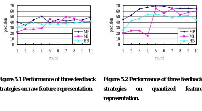
本計畫的研究重點即為利用音樂探勘技術，研究數位音樂典藏中的智慧型擷取技 術。數位音樂典藏的擷取方式包括以後設資料(metadata)查詢、音樂內容擷取, 音樂曲風 查詢, 相關回饋, 音樂瀏覽與個人化音樂推薦等，以有助於使用者方便地擷取典藏的數 位音樂。在本計畫中，我們主要目的將研究利用音樂探勘中的使用者概念學習(User’s Concept Learning) 在 相 關 回 饋 上 ， 發 展 以 內 容 主 的 音 樂 查 詢 (Content-based Music Retrieval)技術。 傳統的音樂檢索系統主要在提供使用者特定音樂的查詢(target search)。除此之外， 使用者也有類型音樂查詢(category search)的需求。在類型音樂查詢中，該類型的所有音 都共同具備使用者所定義的概念(semantic concept)。這個由使用者定義的概念在音樂檢 索系統上是主觀的且動態產生的。換句話說，同一使用者在不同情境之下對於同一首音 樂可能產生不同的解讀概念。為了動態擷取使用者的概念，讓使用者參與在查詢過程的 互動機制是必要的。因此， 我們提出將相關回饋(relevance feedback)的機制運用在以內 容為主的音樂查詢系統上，讓系統從使用者的相關回饋中學習使用者的概念，並利用這 學習出的概念來幫助音樂查詢。 由於使用者可能從整首音樂或音樂片段兩種角度來判斷該音樂是否具備使用者定 義的概念。因此，本論文提出用以片段為主的音樂模型(segment-based modeling approach) 將音樂表示成音樂片段的集合。進一步再從整首音樂和片段中擷取特徵。其次，我們針 對該問題提出相關演算法來探勘使用者的概念。該演算法先從相關和不相關的音樂資料 庫中個別探勘常見樣式，再利用這些樣式建立分類器以區分音樂的相關性。

最後，我們分析各種系統回饋機制對搜尋效果的影響。Most-positive 回傳機制會選 擇根據目前系統判斷為最相關的物件。Most-informative 機制則是回傳系統無法判斷其 相關性的音樂物件。Most-informative 機制的目的在增加每回合系統從使用者身上得到 的資訊量。Hybrid 則是中和前兩種機制的優點。本文中，我們模擬並比較各種回傳機 制的效能。實驗結果顯示相關回饋機制確實能提升查詢的效果。

Data Mining and Intelligent Retrieval Techniques

for Digital Music Archives(Ⅱ)

Abstract

In this project, we investigated the data mining techniques for intelligent retrieval of digital music archive. The way of the digital music archive retrieval, including metadata search, content-based music retrieval, music style retrieval, music browsing, personalized music recommendation and etc., is helpful for retrieving music archive easily. In this project, we utilize the data mining technique to learn user’s concept of relevance feedback for developing content-based music retrieval technique.

Traditional content-based music retrieval system retrieves a specific music object which is similar to the user’s query. There is also a need, category search, for retrieving a specific category of music objects. In category search, music objects of the same category share a common semantic concept which is defined by the user. The concept for category search in music retrieval is subjective and dynamic. Different users at different time may have different interpretations for the same music object. In the music retrieval system along with relevance feedback mechanism, users are expected to be involved in the concept learning process. Relevance feedback enables the system to learn user’s concept dynamically.

In this project, the relevance feedback mechanism for category search of music retrieval based on the semantic concept learning is investigated. We proposed a segment-based music representation to assist the system in discovering user’s concept in terms of low-level music features. Each music object is modeled as a set of significant motivic patterns (SMP) achieved

by discovering motivic repeating pattern. Both global and local music features are considered in concept learning.

Moreover, to discover user’s semantic concept, a two-phase frequent pattern mining algorithm is proposed to discover common properties from relevant and irrelevant objects respectively and based on which a classifier is derived for distinguishing music objects.

Except user’s feedback, three strategies of the system’s feedback to select objects for user’s relevance judgment are investigated. Most-positive strategy returns the most relevant music object to the user while most-informative strategy returns the most uncertain music objects for improving the discrimination power of the next round. Hybrid feedback strategy returns both of them. Comparative experiments are conducted to evaluate effectiveness of the proposed relevance feedback mechanism. Experimental results show that a better precision can be achieved via proposed relevance feedback mechanism.

TABLE OF CONTENTS

ABSTRACT IN CHINESE...i

ABSTRACT ... iii

TABLE OF CONTENTS ...v

LIST OF TABLES ... vii

LIST OF FIGURES ... viii

CHAPTER 1 Introduction ...1

CHAPTER 2 Related Work ...6

2.1 Relevance Feedback Schemes...6

2.2 Music Information Retrieval ...12

CHAPTER 3 Music Object Modeling ...15

3.1 Motivic Repeating Pattern Finding ...…………..16

3.2 Feature Extraction ... ………..20

3.3 Significant Motive Selection... ………..22

CHAPTER 4 Semantic Concept Learning from User’s Relevance

Feedback……...………..24

4.1 Frequent Pattern Mining………..24

4.2 Associative Classification ...31

4.3 S2U Feedback Strategy ...33

CHAPTER 5 Experimental Result and Analysis ...35

5.1 Dataset ...35

5.3 Effectiveness Analysis...36

5.3.1 Effectiveness of System Feedback Strategy...37

5.3.2 Effectiveness of Number of Music Objects Accumulated From

User’s Feedback ...40

5.3.3 Effectiveness of Number of Rounds Applied MI Strategy ...44

5.3.4 Effectiveness of Support and Motive Threshold...45

CHAPTER 6 Conclusions...49

LIST OF TABLES

Table 3.1: An example of correlative matrix...18

Table 3.2: Global and local featrues considered in our work ...21

Table 3.3: Representation of the global feature and three SMPs of the music

object M...23

Table 4.1: An example of MDB

P

...26

Table 4.2: An example of MDB

N

...27

LIST OF FIGURES

Figure 1.1: Framework of music retrieval along with relevance feedback

mechanism...4

Figure 3.1: Transformation from pitch sequence into pitch interval sequence19

Figure 3.2: Examples of six motivic treatments...23

Figure 3.3: Corresponding score of SMPs in Table 3.3 ...23

Figure 4.1: An example of the classifier ...27

Figure 5.1: Performance of three feedback srategies on raw feature

representation……… ...39

Figure 5.2: Performance of three feedback srategies on quantized feature

representation ...39

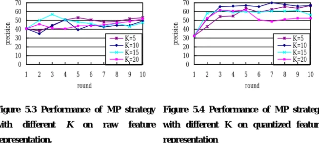
Figure 5.3: Performance of MP srategy with different K on raw feature

representation ...41

Figure 5.4: Performance of MP srategy with different K on quantized feature

representation ...41

Figure 5.5: Performance of MI strategy with different K on raw feature

representation ...42

Figure 5.6: Performance of MI strategy with different K on quantized feature

representation ...42

Figure 5.7: Performance of HB strategy with different K on raw feature

representation ...43

Figure 5.8: Performance of HB strategy with different K on quantized feature

representation ...43

Figure 5.9: Performance of MI strategy with different N on quantized feataure

representation ...44

Figure 5.10: Performance of MP strategy with different motive threshold on

raw feature representation ...46

Figure 5.11: Performance of MP strategy with different motive threshold on

quantized feature representation ...46

Figure 5.12: Performance of MI strategy with different motive threshold on

raw feature representation ...47

Figure 5.13: Performance of MI strategy with different motive threshold on

quantized feature representation ...47

Figure 5.14: Performance of HB strategy with different motive threshold on

raw feature representation ...47

Figure 5.15: Performance of HB strategy with different motive threshold on

CHAPTER 1

Introduction

The amount of digital multimedia data increases with the advances in multimedia and computer technologies. Digital data enriches our lives and technologies for storing, analyzing and accessing multimedia data are increasingly demanded. One of the technologies is multimedia information retrieval which has been conducted for many years. In the area of music retrieval, a typical music retrieval system can discover what user needs by given keywords such as title, author name etc. Except querying by metadata, a content-based retrieval (CBMR) system is introduced which searches for music object by analyzing music content. Traditional content-based music retrieval system discover a specific music object which is similar to a given music segment. Issues related to CBMR include music representation, similarity metric, indexing and query processing.

Instead of searching for a particular music object (“target search”), there is a need for retrieving a specific category of music objects (“category search”). These music objects, of the same category, share a common semantic concept which is defined by the user. For example, when a user wishes to search for romantic music, the retrieved music objects should share the common concept of romantic feeling.

Different users at different time may have established different interpretations of concept for the same music object. Therefore, the concept for category search in music retrieval is subjective and dynamic. The taxonomy of categories of music objects with respect to user’s

concept can’t be constructed in advance and in a fixed way.

To attack this problem, an on-line and user-dependent learning process is needed. Users are expected to be involved in the learning process for two reasons. One is the system lacks of prior knowledge with respect to user’s concept and thus users are required to provide examples. The other is that owing to the scarcity of training samples, relevance feedback provided by the user is needed to improve the retrieval results. In a query session of music retrieval, the process may proceed for several iterations until the user satisfies the result. User’s relevance feedback in each round enables the system to learn user’s concept dynamically. The system accumulates relevance feedback data throughout the session. The performance is expected to be improved via relevance feedback.

In this report, the relevance feedback mechanism for category search of music retrieval based on the semantic concept learning is investigated.There are four main contributions in our work. The first is the investigation of relevance feedback in content-based music retrieval. Little attention has been paid to the design of relevance feedback approach while in content-based music retrieval most users are frustrated in specification of music query.

The second is the proposed segment-based music modeling approach. In traditional multimedia retrieval, most research on relevance feedback approaches models the multimedia object as a whole. Some approaches in image retrieval extended to deal with local features by decomposing an image into regions. In music retrieval, for the sake that concept may be constituted by entire music object or only parts of it, we propose the segment-based music representation to facilitate the system to capture user’s concept in compound granule. In our approach, a music object is treated as a whole as well as a set of music segments. These music segments are extracted from a music object based on music theory.

The third contribution is the developed algorithm for learning user’s semantic concept. The algorithm is presented to enable a learning process based on the segment-based music representation and to discover the concept which is constituted by different music features. We transform the relevance feedback problem to the binary classification problem where examples from user’s feedback are regarded as either irrelevant or relevant to the user’s concept. An on-line and user-dependent classifier is trained to classify music objects from music archive and return the result to the user.

The last one is a comparative performance is evaluated based on three system feedback strategies for returning results for user’s feedback. The strategy adopted will determine how much discrimination power the system can obtain for the next iteration. Most-positive

strategy will return the most relevant music object to the user, most-informative strategy

will return uncertain music objects that provide more discriminative information for systems to learn user’s concept, and hybrid feedback strategies (HB) returns both of them. Traditional method (most positive strategy) always returns the most relevant music objects to the user. Most-informative will select a set of music objects such that user’s feedback will improve the discrimination of uncertain music objects at the next iteration. The strategy highly depends on user’s willingness to interact with the system. For impatient users, the system should applied MP strategy. On the contrary, if users are willing to interact with the system, MI strategy can be applied. The hybrid one is compromise of these two.

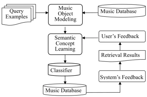
Figure 1.1 illustrates the music retrieval along with the relevance feedback mechanism. Music objects in music archive and user’s example query music are preprocessed by the music object modeling module. The semantic concept learning module is designed to discover from user’s relevance feedback the relationships between user’s semantic concept and music features. A classifier with respect to the user’s relevance concept is derived to classify each

music object in the music archive either as relevant or irrelevant for the next round. The system then will select a collection of music objects for user’s relevance judgment and based on which a further semantic learning process may proceed again once the user isn’t satisfied with the retrieval result. Therefore, a query session may involve more than one rounds of learning process. In each round, there are two types of feedback, the feedback (relevance feedback) given from users to systems (U2S) and the feedback (search result) returned from systems to users (S2U). In the U2S feedback, the user judges each retrieved music object either relevant or irrelevant to the concept. The system proceeds to learn user’s semantic concept from U2S feedback and then returns a collection of music objects for user’s relevance judgment.

Figure 1.1 Framework of music retrieval along with relevance feedback mechanism.

This report is organized as follows. Related work about relevance feedback and music retrieval is introduced in section 2. The music modeling approach is described in section 3.

Semantic Concept Learning Classifier User’s Feedback System’s Feedback Retrieval Results Music Database Query Examples Music Object Modeling Music Database

Section 4 presents the semantic concept learning task. Experimental results are presented in section 5. We conclude our work in section 6.

CHAPTER 2

Related Work

2.1 Relevance feedback schemes

In the area of modern information retrieval, a variety of approaches were developed for improving query formulation through query expansion and term reweighting [20]. Relevance feedback (RF) in image and video retrieval area has been addressed a lot. Most of them extend RF techniques in text retrieval while some of them adopt machine learning techniques. Note that all the existing work may have different assumption and problem settings. In this section, we will list some major variants in different conceptual dimensions in the aspect of user behavior model and algorithmic assumptions.

Object

According to the target that the user looks for, relevance feedback work can be categorized into two types, category search, and target search. In content-based image retrieval (CBIR), most of the work assumes the user is looking for a specific category of images. On the other hand, Cox et al. [4] assume what user looks for is a particular target object and a Bayesian framework is used to evaluate underlying probabilistic distribution over test data in a database via user’s relevance feedback.

Feedback Algorithm

list will be returned to the user based on the system’s RF algorithm. RF algorithm is developed based on defined query representation along with distance function. A typical RF technique which takes user’s relevance judgment into account to provide an improved retrieval results is the query reformulation approach. In [18], two main query reformulation approaches, single-point and multipoint, in single feature representation feedback are mentioned. The well-known technique of single point approach is query point movement (QPM). The objective of QPM approach is to reformulate a new query point such that this new point is close to relevant results and far from irrelevant results. In QPM, a single query is used and regarded as a point in a multidimensional space along with a single distance function (e.g. Euclidean distance function). Multipoint approach opposite to single query point uses multiple query points and aggregate their individual distances to data points into an overall distance. A well known approach is multipoint query expansion (QE). In such paradigm, the objective is to search for objects similar to more than one example. The distance of an object to the query points in a feature space is measured based on a weighted summation of the distances to each query point. When the new multiple query points are constructed through relevance feedback, the membership of the query points and weight that correspond to each query point may be changed. In other words, work adopts QE approach not only reformulate the query by adding new relevant examples or eliminating irrelevant examples but also adjusting weight of each example in each iteration. On the other hand, instead of representing the query in a single multidimensional space, multifeature representation feedback treats each feature representation individually. The query is represented as a collection of single-feature representation queries and an aggregation function is employed to combine the individual query distances into an overall distance. During a query session, the user can select feature representations that he is interested in along with the RF approach for each single feature representation. For example, users can give a query by selecting color histogram

representation using QPM approach for RF and the wavelet feature representation using a multipoint query expansion for RF. A query based on the multifeature query model may be modified by adding or deleting single-feature representation queries and by updating the weights for each single feature query, which is known as query reweighting. Work relative to multifeature representation feedback can refer to [21]. Eventually, an ordered set of multimedia objects will be returned to the user by decreasing relevance by using RF techniques mentioned above.

Research of content-based video retrieval focused on formulating appropriate query via interaction has also been presented in [2] where not only features but also multiple modalities are considered. Information of video objects is implicitly represented by many modalities such as audio, color, and motion vectors. To search a collection of multimedia object is more challenging than searching text documents where natural human language is used to represent a query. Therefore, Amir et. al. [2] probed into a question of what modalities compose of user’s information need when retrieving video objects and presented a mechanism to transform an abstract information need into a concrete search query by using mutual relevance feedback. A query expansion task across multiple modalities proceeds along a query session and will formulate a proper query at the end of a query session. Finally, the multimodal search query will be kept as a meta-representation of the corresponding semantic concept and may be applied later for the same concept without going through tiring interactions again.

Recent work on RF treat it as a classification problem [8][10][22][25][28][28][30]. In classification paradigm, user’s relevance feedback is regarded either as relevant class or irrelevant class and the objective is to incorporate user’s relevance feedback for building classifiers to classify multimedia objects. Most of the previous work utilizes support vector machines (SVMs). Since the SVMs not only set up a decision boundary between relevant and

irrelevant images but also provides a mechanism to rank all of them. Moreover, it’s efficient in facilitating interactions in an on-line environment although it lacks of incremental learning property. In addition to SVMs, some work adopts Bayesian framework [4] and some may use boosting technique to build a composite classifier to make binary decision on each returned objects. For instance, [30] proposed two online pattern classification methods, called interactive random forest (IRF) and adaptive random forests (ARF) which form a composite classier known as random forest for relevance feedback. Both improve the performance of regular random forests in different aspect. IRF improves the efficiency by using a two-level resampling technique, while ARF improves the effectiveness by using dynamic feature extraction and adaptive sample selection techniques.

In addition to classification approach, Yan [32] also mentioned the issue of selecting negative examples since negative instances are less well-defined as a coherent subset. [32] presented a negative pseudo-relevance feedback mechanism which uses the bottom-ranked examples for negative feedback identified based on a similarity metric. The training examples containing the positive examples (the query images) and the negative examples are then fed back to train a margin-based classifier. An adaptive similarity space will be learned following the pseudo-relevance feedback mechanism.

User’s Feedback

There are three main ways for user to provide relevance feedback. The first one is binary feedback where the user judges each returned object either as relevant (or positive) or irrelevant (negative). The second type is degree of (ir)relevance where the user has to score each returned object showing how (ir)relevant an object is with respect to his semantic concept. In this way, it’s difficult and burdensome for users to give (ir)relevance degree for each object consistently. The third type of feedback is a comparative judgment where no

definite relevant and irrelevant judgment is made. Some feedback algorithms may take both positive and negative samples into account while some only consider positive samples.

System’s Feedback

In addition to machine learning technique introduced in RF to increase the discrimination power, an active learning technique related to returning strategy is introduced to improve the discrimination of uncertain object in the next round. It’s a strategy of selecting the best set of object at a feedback round to maximize potential information from the user. A standard strategy always returns the most positive objects based on previous training process. On the other hand, the system can actively query the user for labels to achieve the maximal information. The objects whose labels the system most uncertain about are named most informative objects in [33].

Representation

Most work on CBIR tends to model an image object as a vector in a multiple feature space [18][21]. Each feature dimension will be assigned a feature weight to represent the importance of that dimension. Hence, the feature weight of all dimensions forms a feature weight vector. The goal of algorithms using vector representation is to adjust the weight vector dynamically which may captures user’s interest more precisely via few rounds of feedback learning.

Instead of describing an object as a whole, some work concerns local properties of an object and model an object as a set of feature vector corresponding to a local part. Owing to different expectations of the user, the user may mark an object relevant either based on global or local properties among the object. In some applications, such as [13][14], an image is considered as a set of regions and the system should be capable of leaning regions which are

emphasized by the user if user’s feedback is concerned based on region properties.

Long/Short-Term Learning

Much research about CBIR on RF has been addressed by using machine learning techniques [28][31]. Most learning method only concerns about the feedback information during the current query session. In addition to short-term information, [8][10] also took the knowledge from the past user interactions into account. The learning technique which takes information within the current query session into account is named as short-term learning, while long-term learning will learn knowledge over many query sessions. The function of different learning techniques is slightly different. Short-term learning aims to improve the retrieval result of the current query session and has more flexibility to fit user’s need. On the contrary, long-term learning collects knowledge from the past and aims to boost performance of future sessions. However, the user may have different interpretation for the identical object at different circumstances and hence the past information doesn’t help all the time.

The framework proposed in [8] demonstrated how long-term learning is incorporated into short-term learning in. He et. al [8] proposed a long-term learning approach for constructing a semantic space from user’s past interaction and image content. The high-level semantic space is updated when more and more queries is made. During short-term learning in a query session, the low-level features of the query are extracted to conduct the first round of the retrieval. After that, the system uses the feedback examples to form the semantic representation of the query example. The query is refined and a classifier is generated to differentiate semantically relevant object from irrelevant ones. Then, the user judges the refined retrieval results and the system keeps on next round of short-term learning process if it’s necessary.

2.2 Music Information Retrieval

A traditional information retrieval system aims to search for a particular music object which is close to a rough excerpt of the particular music given by the user. It belongs to the target search problem where key issues include music representation, similarity measure, indexing and query processing techniques [12][17][23]. A typical model of MIR system extracts low-level features (rhythm, melody, chords) from a music object and represents each music object as feature strings. After that, exact or approximate matching process is performed between query object and each one in database. A similarity measure will be addressed in a system allowing approximate matching based on music theory or heuristic rules. On the other hand, in order to speed up the searching process, issues related to index music objects in database may also be conducted.

Relevant research related to music information retrieval includes music recommendation and filtering systems [3][5][15][19][24]. Some of them recommend music object via collaborative filtering technique. Lack of objective similarity metric between multimedia objects has complicated many multimedia applications. When there is no nature idea of similarity between music objects, collaborative filtering strategy seems helpful for prediction. However, the similarity recommendations created by analyzing behaviors and ratings of users do not necessarily correspond to actual music similarity. Besides, popular music objects may dominate the recommendation result.

Chen [3] analyzes polyphonic music object and properly group music objects according to extracted music features and content-based, collaborative and statistics-based recommendation methods are proposed based on the favorite degrees of users to the music groups. Ringo [24] is one of the earliest proposed music recommendation systems by collaborative filtering method. Users are grouped by similar preference and music objects are

recommended based on ratings derived from the users with similar preference. Ragno [19] presented a graph-based preference modeling framework where preference is derived from learning an expertly authored stream (EAS) from radio stations. EAS provides similarities among music objects judged by experts. Based on EAS, the burden of defining similarity metrics by content is avoided. However, the system may always generate same playlists for the same seed song which lack of desirable variety.

Music recommendation can be solved via categorizing music objects by user’s preference. M. Grimaldi et al. [5] used classification approach to predict user’s taste. An instance based classifiers based on user profiles is applied to learn music preferences. In his work, a reasonable accuracy can be achieved if user’s taste is driven by a certain genre preference. A personalized music recommendation system proposed by Kuo [15] use associative classification methods to learn user’s preference based on chords which are extracted from MIDI files. A user’s profile was constructed by marking a sub set of music genre that a user is interested in.

Research about RF in music information retrieval has seldom been conducted. The first work on content-based music information retrieval based on RF was presented in [11]. In Hoshi’s research, a music retrieval system was proposed for searching music objects based on user’s preference. He assumes that the system only has insufficient knowledge about a user’s preference in real world and proposed a retrieval method based on vector representation to address this problem. The user may not be satisfied with the retrieval results which are produced based on insufficient learning data. A relevance feedback mechanism is applied to improve retrieval result and experiments were conducted to show its effectiveness. An advantage of this approach is that it enables the user to discover new songs according to user’s preference. Hoashi also presented two types of profile constructed from user ratings

and from genre preference respectively. Comparative experiments show that precision of user rating based profiles is higher then that of the genre based profiles. When relevance feedback is conducted, genre based method outperforms user rating based method.

CHAPTER 3

Music Object Modeling

A good music representation should be able to assist the system in capturing user’s semantic concept in terms of low-level music features. A music object can be characterized by multiple features such as tempo, rhythm, melody etc. Each feature can be represented as a set of representations. For example, average pitch difference and pitch standard deviations can be used for representations of the melody feature. In the representation space, the semantic concept can be characterized as a subset of representations which discriminates the concept from others. For instance, an inspiring music which rise and fall seriously in melody is describable by average pitch difference.

To understand user’s concept, global features corresponding to an entire objects and

local features with respect to each music segment should be considered. A music object is

composed of a set of music segments. A music object can be globally described by a set of representations in feature space or locally described as multiple sets of representations in feature space where each representation set corresponds to a music segment.

We proposed a segment-based music modeling technique to represent music object in segment level. In our work, the modeling approach consists of three steps. In the first step we represent each music object as a set of segments found by the motivic repeating pattern finding algorithm. Then, multiple feature representations are extracted from each music segment. Moreover, global feature representations are also extracted from an entire music

object to represent the music object as a whole. The last step is to filter significant motivic patterns based on frequency of patterns.

The music modeling approach is organized as follows. Section 3.1 describes the technique for finding motivic repeating patterns. Section 3.2 introduces the step of feature extraction. After that, section 3.3 introduces how to filter significant motivic repeating patterns.

3.1 Motivic Repeating Pattern Finding

In music, a motive is a salient recurring fragment of notes that may be used to construct the entirely or parts of complete melodies and themes. Therefore, each music object can be described by a set of motives. The recurrence of a motive may not be an exact repetition in the music object but with some variations. This is called as motivic treatment in musicology [26]. Six common motivic treatments (a)repetition (exact repeat), (b)transpose (interval repeat), (c)sequence, (d)contrary motion, (e)retrograde, and (f)augmentation/ diminution repetition are considered in our work (Figure 3.1).

We first apply the all-mono method to extract main melody. The extracted main melody will be represented as a note sequence where each note is expressed by pitch and its duration. Then, we modified the correlative matrix method [12], originally designed for exact repeating pattern finding, to discover six variations of motivic repetitions [9]. Finally, a minimum constraint on the length of a fragment is used to retain motivic patterns of more than four notes.

The correlative matrix method is utilized for repeating pattern discovery with a given note sequence. It includes the following three steps:

1) Construct Correlative Matrix:

The correlative matrix is the data structure which is initially formed by the given note sequence. Namely, if the length of note sequence is n, the size of the matrix is nxn. The purpose of the first step is to fill the matrix row by row. For the ith note and the

jth note in the note sequence, the cell of ith row and the jth column in the matrix will be set as one if they are the same, otherwise it will be empty. In addition to the current matching results, the value of cell in the ith row and the jth column is also decided based on the result of the cell in the (i-1)th row and (j-1)th column. Assume the value of the cell in (i-1)th row and (j-1)th column is v. The value of the cell in ith row and jth column will be set to v+1 if the ith note is the same as jth note in the sequence. The value in the cell indicates the length of a potential repetition.

After the construction step, the matrix will keep all of the intermediate results of substring matching.

2) Find Candidate Set:

For each non-empty cell, the corresponding pattern is regarded as a candidate, a potential repeating pattern. The associated information is computed as we find each candidate. The information includes, pattern, rep_count, and sub_count. Pattern indicates the repeating pattern, rep_count represents the count of matching for the repeating pattern, and sub_count means the number of other repeating patterns which contains this pattern. To calculate the rep_count and sub_count for the ith row and jth column (Mij), conditions of Mi-1,j-1 and Mi+1, j+1 has be taken into account. After computation for each non-empty cell, patterns with their corresponding repetition count and substring count will be used to calculate pattern frequency in the next step. 3) Discover Non-trivial Repeating Patterns:

The purpose of this step is to discover all non-trivial repeating patterns and calculate the actual frequency of each legal pattern. A pattern is trivial if its rep_count equals

sub_count. The trivial case indicates that there exists a superstring S’ containing the

pattern S and S appears along with S’. In such case, the superstring S’ is considered more representative and hence the trivial pattern S will be removed. After removal, the frequency f of each pattern p in a music object m is calculated by the formula:

2 ) _ 8 1 1 ( ) , (p m rep count f = + + × (1)

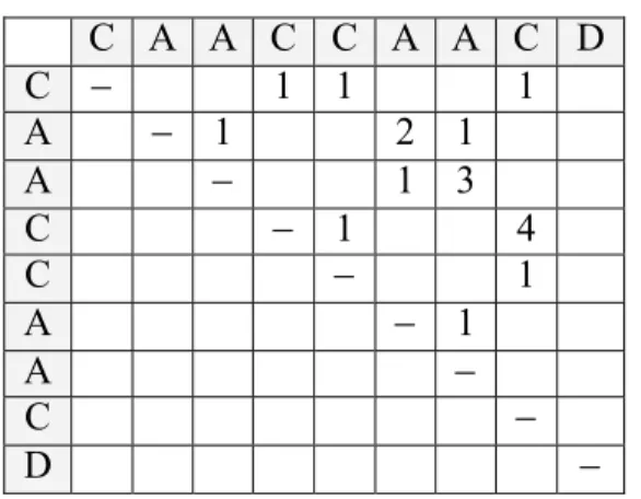
Table 3.1 shows an example. Given a note sequence of “CAACCAACD”, the correlative matrix is constructed by substring matching row by row. For the 1st note “C”, it repeats in 4th, 5th, and 8th position of the sequence. For the cell M26, because “A” in the 2nd row matches the “A" in the 6th column and M15 is 1, the value of M26 is set to 2. The value 2 indicates the

pattern “CA” with length 2. To find all candidates, all non-empty cells is scanned and associated information of each candidate is computed. Take M37 as an example. The corresponding pattern of M37 is “CAA”, whose count of match so far is one and is a substring of the pattern “CAAC” since M48 isn’t empty. Hence, the associated information of “CAA” is (“CAA”, 1, 1). Since the rep_count of “CAA” equals sub_count, “CAA” is a trivial pattern and will be removed. The pattern “C” is an example of non-trivial patterns.

Table 3.1 An example of correlative matrix.

C A A C C A A C D C − 1 1 1 A − 1 2 1 A − 1 3 C − 1 4 C − 1 A − 1 A − C − D −

The method described is the standard version for discovering exact repeating patterns and can’t be applied for other repeating variants shows in Figure 3.1 without modification. For exact repetition (Figure 3.1 (a)), we can utilize the method directly.

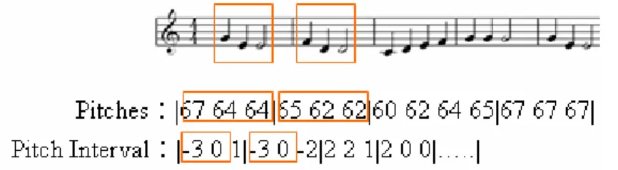
For transpose (interval repeat) (Figure 3.2 (b)), we have to transform the pitch sequence into pitch interval sequence(Figure 3.1). After that, the correlative matrix method is applied on the pitch interval sequence.

Figure 3.1 Transformation from pitch sequence into pitch interval sequence.

Sequence is a type of motive treatment which contains more than three consecutive motive transpositions (Figure 3.2 (c)). Beside, the direction of the transposition has to be the same, namely ascending or descending. In Figure 3.2 (c), the first rectangle indicates the original motive. The second and third are the transposition of the original motive. To discover sequence, the method is the same as the case of transpose except that we have to check whether the discovered pattern is repeated consecutively.

Contrary motion (Figure 3.2 (d)) is a motive treatment where pitch interval sequence is inversely repeated while the rhythm keeps the same. Namely, the contrary motion of the original motive can be obtained by assigning opposite sign for each pitch interval. To discover contrary motion, the correlative matrix is constructed by two different sequences. One is the original pitch interval sequence and the other is the one with opposite sign. Others remain the same.

Retrograde is a repetition where pitch contour is inversely repeated while rhythm keeps the same. Figure 3.2 (e) gives an example. The second motive <72, 72, 71, 67, 65, 65> is the retrograde of the first one <65, 65, 67, 71, 72, 72>. To discover retrograde in the sequence, The conditions to decide the value for each cell is changed. To assign the value of Mij, the original method will take Mi-1,j-1 into account while Mi-1,j+1 will be considered in the retrograde case. Others remain the same.

Augmentation (diminution) repetition is repetition where pitch sequence remains the same while rhythm becomes faster (slower) with a ratio. In Figure 3.2 (f), the second motive is the augmentation repetition of the first one and the third motive is the diminution of the first one. To discover augmentation (diminution) repetition, the process for discovering repeating patterns remains the same while an additional check on the results is needed to ensure the rhythm of repetitions with regarded to one pattern is changed in a ratio.

After six discovery processes perform on each music object, we only keep original motive to represent the structure feature of that music. Next step describes the process of feature extraction.

3.2 Feature Extraction

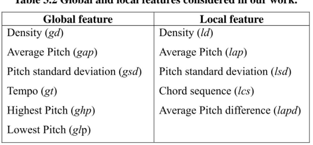
We extract six kinds of global feature representation and five kinds of local feature representation shown in Table 3.2. In other words, each music object is modeled as a six-attribute global feature and a set of five-attribute local features. Music features considered in this report are melody, rhythm and tempo. Representations for melody features include average pitch, pitch standard deviation, highest/lowest pitch, chord sequence and average pitch difference. Rhythm feature is represented as density while tempo is represented as the tempo value only.

Average pitch is the average pitch values of notes within a music piece (an entire one or a segment). Pitch standard deviation is the standard deviation of pitch values of notes within a music piece. Highest and lowest pitch value is extracted from a music object and average pitch difference indicates the average of difference in pitch between two consecutive notes within a music segment. Chord sequence is a sequence of chord within a segment calculated by chord assignment algorithm which is a heuristic method based on harmony and music theory. Details on chord sequence can be seen in [14]. Density of a music piece is defined as number of notes dividing by the total duration of a music piece. Tempo denotes the speed of a music object and is defined as number of beats per minute.

Table 3.2 Global and local features considered in our work. Global feature Local feature

Density (gd)

Average Pitch (gap)

Pitch standard deviation (gsd) Tempo (gt)

Highest Pitch (ghp) Lowest Pitch (glp)

Density (ld)

Average Pitch (lap)

Pitch standard deviation (lsd) Chord sequence (lcs)

Average Pitch difference (lapd)

In some cases, two different music segments may be approximately sounds the same. In order to consider the fault-tolerant cases, we intent to quantize the feature values in each segment. In the aspect of global feature, density and pitch standard deviation are quantized by the range of 0.5. More precisely, the quantized value will equal the quotient obtained by dividing the raw value by 0.5. For instance, two densities of 1.7 and 1.9 are quantized as 3. In the same way, the average pitch, highest pitch and lowest pitch are divided by 5. In the part of local feature, density, pitch standard deviation and average pitch difference are divided by 0.5.

The average pitch value is quantized as it does in the global feature, while the chord sequence remains the original value.

In order to observe the impact of quantization on performance, we keep two copies of features, the raw one and the quantized one. These two copies will be processed in the next step and the sequential learning process respectively. We will compare the performance of the two different representations in the chapter 5.

3.1 Significant Motive Selection

We aim to filter significant motivic patterns (SMPs) in this step. We measure the significance of each motivic repeating pattern and retain those significant one with regard to a music segment. A motivic repeating pattern with high frequency in the music object isn’t necessarily more important than the one with low frequency in the other music object. Therefore, the frequency of a motive, f(p,m), is normalized by dividing the maximal frequency of the motivic pattern p’ in music m. A motive is more important with respect to one music object if the motive is more specific in the music database (DB) and thus the importance of a motive with respect to one music object is defined as follows:

) , sup( ) ,' ( max ) , ( ) , ( ' DB p m p f m p f m p W = p∈m (2)

where sup(p,DB) stands for the support of p in the DB.

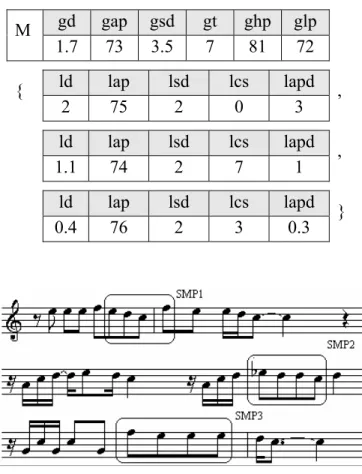
Table 3.3 shows the representations of the song “don’t let the sun go down on me” which contains eight SMPs with importance higher than 0.5. Only the representations of global feature and local features of three SMPs are shown in Table 3.2. Figure 3.3 illustrate the corresponding score for these SMPs.

Figure 3.2 Examples of six motivic treatments.

Table 3.3 Representation of the global feature and three SMPs of the music object M.

gd gap gsd gt ghp glp M 1.7 73 3.5 7 81 72 ld lap lsd lcs lapd { 2 75 2 0 3 , ld lap lsd lcs lapd 1.1 74 2 7 1 , ld lap lsd lcs lapd 0.4 76 2 3 0.3 }

CHAPTER 4

Semantic Learning from User’s Relevance Feedback

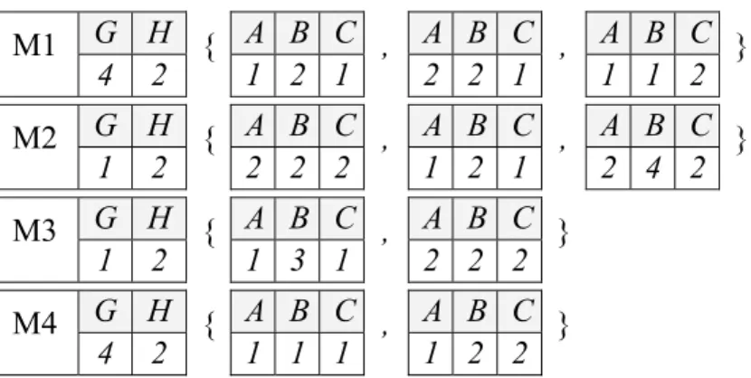
The semantic learning process at each round is performed on the accumulated training data. The training data is composed of two databases, the relevant one (MDBP) and irrelevant one (MDBN). Each database contains relevant/irrelevant music objects accumulated from previous rounds. The amount of samples in each MDBP/ MDBN increases during the session. The concept can be learned by mining common properties of MDBP andMDBN respectively first and then discovering discrimination between these properties. Table 4.1 is an example of MDBP containing four music objects while Table 4.2 is an example of MDBN with three music objects. For convenience of explanations, in these examples, a music object is modeled as a two-attribute global feature (G, H), and a set of three-attribute local features (A, B, C) where each three-attribute local feature corresponding to a SMP. One example of common properties of MDBP is (A=1,C=1) and one example of discriminative properties of MDBP and MDBN is (B=2) & (H=2) & (A=1, C=1) which appears frequently in MDBP but seldom or never appears in MDBN.

The semantic learning process for capturing user’s concept proceeds first by frequent pattern mining algorithm followed by associated classification algorithm. Details are shown in the following.

Relevance/irrelevance is usually defined by a characteristic that is shard by relevant/irrelevant music objects. To capture the characteristic sharing by a class of music objects, we employ the data mining techniques. Before the mining process, each (attribute, value) pair of the global and local feature is transformed to an item. For example, an (attribute, value) pair of (B,2) is transformed to an item “B2”. Therefore, the global feature is represented as an itemset of six items while the local feature of an SMP is represented as an itemset of five items. A music object is therefore treated as a set of itemsets. Before presenting the algorithm, we introduce some formal definitions in the following.

Definition 1:

Let I be the set of possible items and Y = {X| X ⊆ I, X is the itemset corresponding to a local feature or a global feature}. Let MDBP/MDBN be a music database, where each object T is a set of itemset such that T={T1, T2,…,Tx| Ti∈Y }, namely T ⊆Y.

Example 1:

Take M1 in table 4.1 as an example. The object M1 is represented as {{G4, H2}, {A1, B2,

C1}, {A2, B2, C1}, {A1, B1, C2}}.

The common property found in this mining stage is called a frequent pattern,.

Definition 2:

Let X be the itemset corresponding to a local feature or a global feature. The common property, pattern, found in the mining stage is a set of itmest, P = {P1, P2,…,Pv| Pj ⊆ X }.

Example 2:

An example of pattern in table 3 is {{H2}, {A1,C1}} where itemset {H2} and {A1, C1} are the subset of a local feature or a global feature.

Definition 3:

We say that an object T contains the pattern P if there is a one-to-one mapping function from

P to T such that for each Pi, there exists a Ti, Ti∈T ∋ Pi ⊆ Ti.

Example 3:

Take the pattern {{A2}, {C2}} as an example. If an object contains {{A2}, {C2}}, there must exist two distinct itemset containing {A2} and {C2} respectively. For instance, in table 4.1 M1 and M2 contains {{A2}, {C2}}, while M3 doesn’t contain {{A2}, {C2}}.

Definition 4:

Given a pattern P, the support count of P, supCount(P), is the number of objects in MDBP / MDBN that contain P and it’s support sup(P) in an object database is (supCount(P))*100%. We called P a frequent pattern if sup(P) is no less than a given minimum support threshold ,minsup.

Example 4:

An example of frequent patterns with support 100% in MDBP is {{B2}, {H2}, {A1,C1}} which is contained in all objects in MDBP.

Table 4.1 An example of MDBP. G H A B C A B C A B C M1 4 2 { 1 2 1 , 2 2 1 , 1 1 2 } G H A B C A B C A B C M2 1 2 { 2 2 2 , 1 2 1 , 2 4 2 } G H A B C A B C M3 1 2 { 1 3 1 , 2 2 2 } G H A B C A B C M4 4 2 { 1 1 1 , 1 2 2 }

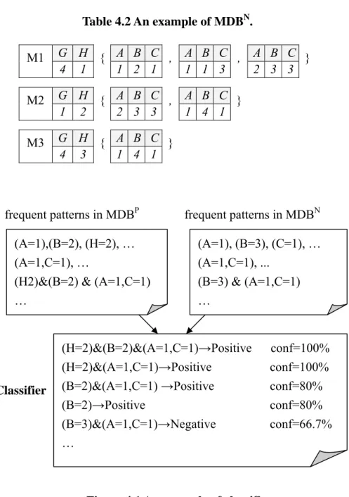
Table 4.2 An example of MDBN. G H A B C A B C A B C M1 4 1 { 1 2 1 , 1 1 3 , 2 3 3 } G H A B C A B C M2 1 2 { 2 3 3 , 1 4 1 } G H A B C M3 4 3 { 1 4 1 }

Figure 4.1 An example of classifier.

The task of frequent pattern mining is to find all frequent patterns with support no less than the minimum support threshold minsup. The frequent pattern found in MDBP, MDBN are called positive frequent pattern and negative frequent pattern respectively. Both of them are is the form of set of itemsets.

A well-known approach for mining frequent pattern is Apriori algorithm [1]. Apriori is a frequent patterns in MDBP

(A=1),(B=2), (H=2), … (A=1,C=1), …

(H2)&(B=2) & (A=1,C=1) … frequent patterns in MDBN (A=1), (B=3), (C=1), … (A=1,C=1), ... (B=3) & (A=1,C=1) … (H=2)&(B=2)&(A=1,C=1)→Positive conf=100% (H=2)&(A=1,C=1)→Positive conf=100% (B=2)&(A=1,C=1) →Positive conf=80% (B=2)→Positive conf=80% (B=3)&(A=1,C=1)→Negative conf=66.7% …

data mining technique originally developed to discover frequent itemsets from database of itemsets. However, in our work, MDBP/MDBN.is a database of sets of itemsets and the frequent pattern is also a set of itemsets. Therefore, we proposed a two-phase mining algorithm modified from Apriori to discover the frequent patterns. The first phase will find the frequent itemsets and the second phase will discover the frequent patterns constituted by the frequent itemset found in the first phase. Note that the itemset found in the first phase corresponds to the music segment (SMP) level while the pattern (set of itemsets) found in the second phase corresponds to the music object level. The mining process will proceed on both MDBP and MDBN respectively.

1st phase : mining frequent itemsets

We employ Apriori algorithm to discover all frequent itemset in which each item must appear in the same itemset. The classic Apriori algorithm for discovering frequent itemset makes multiple passes over the database. In the first pass, support of each individual item is calculated and those above the minsup will be kept as a seed set. In the subsequent pass, the seed set is used to generate new potentially frequent itemsets, candidate itemsets. Then the support of each candidate itemset is calculated by scanning the database. Those candidates with support no less than minsup are the frequent itemsets and are fed into the seed set that will be used for the next pass. The process continues until no new frequent itemsets are found. In our work, only the step of support calculation is different from classic Apriori algorithm, since in our work each object is a set of itemset, rather than an itemset. For the example of Table 3, the support count of the frequent itemset {A2, C2} is two. {A2, C2} appears in M2, M3, but not in M1, M4.

2nd phase : mining in segment level

The second phase will discover the patterns constituted by frequent itemsets found in the first phase. Similar to the algorithm in the first phase, the algorithm makes multiple passes over the database MDBP/MDBN. In the k-th pass, the seed set (the set of candidate patterns of

k itemsets) is generated by joining two frequent patterns of k itemsets found in the previous

pass. Then the support of each candidate pattern is calculated by scanning the database. Those candidates with support no less than minsup are the frequent patterns and are fed into the seed set that will be used for the next pass. The process continues until no new frequent patterns are found. The only exception is the first pass in which the seeds are the frequent itemsets generated in the first phase.

In order to improve the efficiency of the above mining process, we introduce the pattern

canonical form in the following to makes the candidate generation more efficient.

Following shows the definitions and examples.

Definition 5:

Let Pk be a pattern containing k itemsets. Assume that items in an itemset is ordered by lexicographic ordering pl. The pattern canonical form of P k is defined as the set of itemsets

in which itemset is rendered based on the ordering _ppcf. We define the ordering _ppcfas follows. If α = {s1, s2, …,sm} and β = {t1, t2, …,tn} are two itemsets in P k, then αppcfβ iff one of the following is true.

(i) m < n or

(ii) m = n and ∃i,j,1<i< j,∋sαk = tβk for 1<k≤i and sαj_plt_βj.

Example 5:

Definition 6:

Given two frequent k-patterns in pattern canonical form, {P1, P2,…,Pk} and {Q1, Q2,…,Qk, they are joinable if P2= Q1 and P3= Q2, …, and Pk = Q(k-1). A (k+1)-candidate pattern {P1,

P2,…, Pk,Qk} will be generated in canonical form as well.

Example 6:

Given two frequent 2-patterns in canonical form, {{A1},{B2}} and {{B2},{A1,C1}} will generate the 3-candidate pattern {{A1},{B2},{A1,C1}}.

Moreover, in order to count the support of patterns more efficiently, we maintain a table,

occurrence table, for each pattern.

Definition 7:

Given a frequent k-patterns P in pattern canonical form, {P1, P2,…,Pk}, the occurrence of P in object T is {LP1, LP2, …, LPk} where LPi, 1 ≦ i ≦ k indicates the location of itemset Piin T. There may be more than one occurrence in an object. The table records all occurrences in each object in the database for P is called the occurrence table.

Example 7:

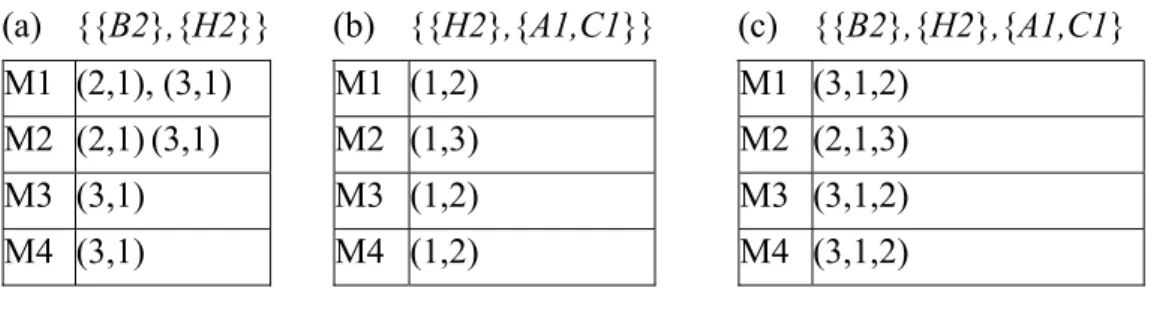
The occurrence tables for the patterns {{B2},{H2}} and {{H2},{A1,C1}} are shown in Table 5(a) and (b) respectively. In Table 5(a), the first occurrence of the pattern {{B2},{H2}} in music object M1 is (2,1) where {B2} appears in the 2nd itemset and {H2} appears in the 1st itemset of music object M1.

We use the data structure, occurrence table, to store positions where the pattern appears in. Each pattern is associated with an occurrence table. Moreover, we also derive the occurrence table for each candidate during the process candidate generation.

Table 4.3 Examples of occurrence tables.

(a) {{B2},{H2}} (b) {{H2},{A1,C1}} (c) {{B2},{H2},{A1,C1} M1 (2,1), (3,1) M1 (1,2) M1 (3,1,2)

M2 (2,1)(3,1) M2 (1,3) M2 (2,1,3)

M3 (3,1) M3 (1,2) M3 (3,1,2)

M4 (3,1) M4 (1,2) M4 (3,1,2)

Definition 8:

Given two joinable k-patterns along with their occurrence tables, suppose that the occurrence of the first pattern in a specific music object is (u1, u2, …,uk) while that of the second pattern in the same music object is (v1, v2, …,vk), an occurrence (u1, u2, …, uk, vk) for this object will be generated if u2= v1, u3= v2,…, uk = v(k-1) and u1 ≠ vk.

Example 8:

Given two occurrence tables in Table 5(a) and 5(b), the occurrence table for the candidate {{B2}, {H2}, {A1,C1}} is presented in Table 5(c). In Table 5(c), the occurrence in object M1, (3,1,2) is generated by (3,1) in Table 5(a) and (1,2)in Table 5(b) of M1.

By utilizing the occurrence table, it is efficient to check the support count of each candidate pattern without scanning the music database.

4.2 Associative Classification

After a two-level mining process performs on MDBP and MDBN,we obtain a collection of positive and negative frequent patterns with respect to the common properties of music objects relevant and irrelevant to the concept respectively. In order to discriminate the concept of relevant music from that of irrelevant music, this step tries to find the discrimination between characteristics of MDBP and MDBN. The result of this step is a classifier consisting

of rules. Figure 4.1 is an example of classifier learned from common properties discovered from Table 3 and 4. One rule is “(B=2) & (A=1,C=1)→ Positive”, which classifies a music object containing attributes of (B=2) &(A=1,C=1) as positive class. This rule comes from the fact that (B=2) & (A=1,C=1) appears frequently in MDBP but seldom appears in MDBN.

We employ associative classification algorithm [16] to generate a binary classifier learned from the positive and negative frequent patterns. The algorithm eventually will generate a classifier containing a set of ranked rules. The classifier is of the form <r1, r1,…, r1,

default_class}. Each rule ri is of the forml⇒y, wherel∈F, F is the collection of positive and

negative frequent patterns and y is a class label. The confidence of a rule is defined as the

percentage of the training music that contains l belonging to class y.

A naïve version of the algorithm will first sort the set of rules according to a defined precedence order. And then select rules following the sorted sequence that correctly classify at least one music object and will be a potential rule in our classifier. Different from the original rule type, the frequent pattern on the left hand side of one rule in our work is a set of itemset. We say that a music object is covered by a rule if it contains the frequent pattern of the rule. Take the rule {{B2},{A1,C1}}→ positive in Figure 4.1 as an example, if a music object has two itemsets containing {B2} and {A1,C1} respectively, then the music objects is covered by rule {{B2},{A1,C1}}→Positive. If the music object is in MDBP, we say that it’s correctly classified by the rule. A default class referred to the majority class of the remaining music object in database is determined. Finally, it will discard those rules that do not improve the accuracy of the classifier. The first rule in classifier that made the least error recorded in classifier is the cut off rule where rules after the cut off rule will be discarded since they only produce more errors.

4.3 S2U Feedback Strategy

Once the classifier is constructed, the system then produces a ranked list of music objects. As we have mentioned in section 1, what the system return to the user will determine the potential information granted from the user. We present three types of feedback strategies, most-positive, most-informative and hybrid strategies. In general, the most-informative music objects will not coincide with the most-positive music objects. Different strategies along with corresponding scoring function are described as follows.

(1) Most-Positive strategy (MP)

If the user is impatient, the system should present the most positive (i.e. those marked as relevant by the system) music objects learned so far. The most positive music is a list of music object m ordered by the score function which is related to the confidence of matched rules.

∑ ∑ = ∪ ∈ ∈ Rn Rp r Rp r MP _{conf r} r conf m Score ) ( ) ( ) ( (3)

where Rp/Rn stands for rules belong to positive/negative class that satisfies each music object

m.

(2) Most-Informative strategy (MI)

If we sacrifice the performance at this round for maximizing information obtained for the next round, a better result can be expected in the future process. Most-Informative strategy will select a set of music objects such that their judgment by the user will provide more information for labeling uncertain music objects. The uncertain music objects are those whose

class labels the system is uncertain about. These objects are most-informative objects. In other word, the system using MI strategy will display a collection of most informative objects at each round until the user attempts to find out what the system can retrieve in hand. Then, the system will adjust itself to MP strategy and return the most positive music objects.

In the associative classification algorithm, object which matches no rules in hand belongs to the default class. We define those belong to default class as most informative music objects. If the user is willing to interact with the system, our system will display a number of most informative music objects for user’s feedback.

(3) Hybrid strategy (HB)

HB is a compromised between MP and MI strategies. The system applied HB strategy will equally return both most positive and most informative objects each round. The score of each music object m is defined as follows:

⎩ ⎨ ⎧ ∈ = otherwise m score class default m m score MP HB _{( ),} _ , 5 . 0 ) ( (4)

CHAPTER 5

Experimental Result and Analysis

5.1 Dataset

The dataset contains 215 MIDI music objects collected from the internet. Each music object belongs to western pop music including rock, jazz, and country genres. Subjects involved in the experiment are unfamiliar with some of the music objects. In this case, noisy and inconsistent judgment caused by the user because of familiarity may be avoided.

Automatic melody extraction process is performed on each MIDI file by all-mono algorithm. The raw feature representation and quantized version will be fed to the system separately for performance evaluation.

5.2 Experiment Setup

In order to evaluate the segment-based relevance feedback algorithm, we design an on-line CBMR system with relevance feedback mechanism. The relevance feedback information of users is essential for system evaluation. We invite eight subjects to investigate our system for creating relevance feedback data.

The retrieval process proceeds by randomly selecting 20 music objects for user’s labeling. An on-line training process will derive a classifier based on initial U2S feedback. The classifier labels all music objects in database along with a scoring function which defines

relevance degree of each one. According to specified S2U feedback strategy, at most 20 music objects will be returned and judged by the user. Once the user isn’t satisfied with the current retrieval result, next round proceeds again. The training samples are accumulated from each relevance feedback round. The classifier is expected to be refined based on the accumulated training samples via the relevance feedback mechanism.

In order to compare with performances for experiments with different strategies and parameter settings, the user has to go through many experiments and provide relevance feedback for each one of them in reality. It wastes user’s time and somewhat a tiring job. To reduce user’s burden, we attempt to collect user’s relevance feedback data in advance. Once the user determines the concept in mind, the user labels each music object in the database either as relevant or irrelevant. The relevance feedback data made by the user will be regarded as the groundtruth. After that, a series of experiments for each user will be conducted. Each experiment corresponding to a query session contains many rounds will be simulated and each returned music object will be automatically label based on user’s groudtruth.

5.3 Effectiveness Analysis

In order to evaluate the results of our experiments, the performance measure employed is based on the average precision, which is defined as the ratio of the number of relevant music objects of the returned music objects over the number of total returned music objects n for all users.

Note that each experiment intends to evaluate effectiveness of the refinement framework on music retrieval system. Music objects that system has returned in previous round will not be removed from the music database.

We conducted four sets of experiments for performance comparison. The first one is to evaluate the different feedback strategies of the system. The second experiment is to measure the effectiveness of the number of music objects accumulated from user’s feedback (top K). Subsequently, the experimental result for evaluating effectiveness of the number of rounds (N) applied most-informative (MI) will be discussed. Finally we show the effect of motive threshold on performance.

5.3.1 Effectiveness of System Feedback Strategy

We perform three different experiments to compare the effectiveness of system feedback strategy applied for each round during a query session. As mentioned in section 4.3, the system can employ MP, MI or HB strategy at each round. Three different experiments are described as follows:

S2U feedback strategy (MP): the system applies MP feedback strategy each round and only uses the top K music objects returned for further refinement.

S2U feedback strategy (MI): the system applies MI feedback strategy for consecutive N rounds and then evaluates the final result by applying MP feedback strategy for the rest of rounds. By examining precision at the N+1 round among three S2U feedback strategies, how well does MI strategy work can be evaluated.

S2U feedback strategy (HB): the system applies HB feedback strategy each round during the query session.