依據品質良率指標Yq應用複式抽樣方法於供應商選擇

國立交通大學

工業工程與管理學系

碩士論文

依據品質良率指標

Y

_q

應用複式抽樣方法於

供應商選擇

Bootstrap Approach for Supplier Selection Based on

Quality Yield Index

Y

_q

研 究 生：郭威麟

指導教授：彭文理 博士

吳建瑋 博士

依據品質良率指標

Y

_q

應用複式抽樣方法於

供應商選擇

Bootstrap Approach for Supplier Selection Based on

Quality Yield Index

Y

_q

研 究 生： 郭威麟 Student : Wei-Lin Kuo 指導教授： 彭文理 博士 Advisor: Dr. W. L. Pearn 吳建瑋 博士 Dr. Chien-Wei Wu

國 立 交 通 大 學

工 業 工 程 與 管 理 學 系

碩 士 論 文

A Thesis

Submitted to Department of Industrial Engineering and Management

College of Management

National Chiao Tung University

in partial Fulfillment of the Requirements

for the Degree of

Master

in

Industrial Engineering

May 2007

Hsinchu, Taiwan, Republic of China

依據品質良率指標

Y

_q

應用複式抽樣方法於

供應商選擇

研究生：郭威麟 指導教授：彭文理 博士

吳建瑋 博士

國立交通大學工業工程與管理學系碩士班

摘要

製程良率 (Process Yield) 仍是應用於製造工業中對於量測製程好壞的一個 判斷標準，而更為先進的量測公式稱為品質良率指標 又將顧客損失考慮在 內。Ng and Tsui 在 1992 年指出品質良率指標針對產品品質特性偏離目標值之變 異程度對良率作一個處罰的動作，即把平均的產品損失考慮出來。本研究應用品 質良率指標來比較兩家供應商的製程能力。我們使用假設檢定來比較兩個指標， 並且改寫成差距 ( , q Y 0: q2 q1 0 H Y −Y ≤ H Y₁: _q2 −Y_q1 >0) 以及比例 ( , ) 的形式分別來作比較。由於抽樣分配較為複雜，因此本研究使 用複式抽樣的模擬方法來建立差距以及比例值的信賴下界。我們也針對了錯誤機 率以及檢定力去比較四種複式抽樣方法間的表現。為了實務上的便利，本研究依 據所需的檢定力整理出建議的樣本數量表並且基於我們建議的方法去設計一個 流程來衡量兩家供應商的品質。最後，我們以一個製造電漿面板產品的製程為 例，套用我們的流程去幫助製造商選擇一個製程品質較好的供應商。 0 : q2/ q1 H Y Y ≤ 1 1 1: q2/ q1 H Y Y > 關鍵字：複式抽樣方法、信賴下界、假設檢定、模擬、供應商選擇、品質良率。

Bootstrap Approach for Supplier Selection Based

on Quality Yield Index

Y

_q

Student:

Wei-Lin

Kuo

Advisor: Dr. W. L. Pearn

Dr. Chien-Wei Wu

Department of Industrial Engineering and Management

National Chiao Tung University

Abstract

Process yield has been used in the manufacturing industry for measuring process performance. A more advanced measurement formula called the quality index , has been proposed to calculate the quality yield for arbitrary processes by taking customer loss into consideration. Ng and Tsui (1992) indicated that penalizes yield for the variation of the product characteristics form its target, which presents a measure of the average product loss. In this paper, we use the index to compare which supplier has better process performance. The supplier selection decisions would be based on the hypothesis testing comparing the two values,

q Y q Y q Y q Y H Y₀: _q2−Y_q1 ≤0 versus H Y₁: _q2−Y_q1>0 (difference

testing), or versus (ratio testing). Due to the

complexity of the sampling probability, we use a bootstrap resampling simulation to construct a lower confidence bound for the difference and the ratio statistics. To compare the performance of those four Bootstrap methods, further simulations of error probability and selection power analysis are conducted. For practical application, we tabulate the different sample size required for designated selecting power. A selection procedure is developed to select a better supplier in quality performance with the method. Finally, we also investigate a real-world case on the PDP (Plasma Display Panel) and apply the selecting procedure to help the manufacturer selecting a better supplier.

0: q2/ q1

H Y Y ≤ 1 H Y₁: _q2/Y >_q1 1

Keywords: Bootstrap methods, Lower confidence bound, Hypothesis testing, Simulation, Supplier selection, Quality yield.

誌謝

終於完成了我人生中的第一本著作。能夠走到現在這一步，一路上承蒙許多 朋友的關心和打氣。首先要多謝彭老師以及吳建瑋老師的指導，對我的論文的架 構以及完整性有了很大的幫助。彭老師常常語重心長的跟我們講很多道理，讓我 對事情有了許多不一樣的看法。還有鍾淑馨老師，在口試時候給了我許多的意見 也讓我獲益不少。學長姐們在我修訂格式以及排版時，也幫了我很多忙。特別感 謝雅靜以及雅甄學姐，抽空幫我指導論文格式以及摘要的寫法。讓我這篇一開始 慘不忍睹的論文，慢慢的有模有樣。 從我一進實驗室以來，我很慶幸我可以遇到一群好同學。耀聰以及阿亮實在 是兩個很積極進取的人，讓我在研究期間深怕追不上兩人的腳步，一起出去吃清 大猪排的時光真是讓人難忘。我覺得我以後一定會常常想起晚上跟阿亮一起改論 文，一邊改一邊為自己的粗心而笑的那段時間。仲軒是一個很奇妙的人，做什麼 事情都是怡然自得的樣子。他的羽球以及唱歌真的蠻厲害的。隔壁研究室的夥 伴，雖然大家相隔兩地，每次吃飯還是不會忘記過來找一下。善康學長以及于婷 學姊，真是我心目中的大哥哥大姐姐，總是可以在我煩惱時給予我一些中肯的建 議。還有我們實驗室的三位學長，百忙之中總是不忘走過來說一些有趣的話題。 碩一的兩位學弟你們好好努力吧，相信你們會有不一樣的收穫。寢室的三位室 友，雖然大家都為論文所苦，可是在宿舍的時光總是一樣的歡樂。 在我研究所的這段時間，我覺得我學會了面對事情的一些觀點。有時候很多 事情會和你想的不一樣。隨著年齡漸漸變大，這種事情會越來越多。這可能是想 法變成熟的開始吧，希望這些經驗可以幫助我以後在社會上保持應有的態度以及 熱情。最後真的要感謝我的老媽，一個人努力工作撫養我長大。等我當完兵後， 就讓我來盡一下孝道吧。 將此論文獻給我親愛的家人以及所有陪伴我的朋友

Contents

摘要...i Abstract...ii 誌謝... iii Contents...iv List of Table ...v List of Figure...vi Notations ... viii 1. Introduction ...1 2. Literature Review ...2

2.1. Process Capability Indices ...2

2.2. Quality Yield Y_q and Relation Indices...3

2.2.1. Process Yield ...3

2.2.2. Process Lose ...4

2.2.3. Quality Yield Y_q ...4

2.3. Investigation in Supplier Selection...5

3. Selection Method ...6

3.1. Selecting a Better Supplier by Comparing Two Y_q Indices...6

3.2. Bootstrap Methodology ...7

4. Performance Comparisons of Four Bootstrap Methods ...11

4.1. Simulation Layout Setting ...11

4.2. Error Probability Analysis...13

4.3. Selection Power Analysis...17

5. Supplier Selection Based on BCPB Method ...19

5.1. Sample Size Determination with Designated Selection Power ...19

5.2. Selecting the Better Supplier ...20

6. Application Example :PDP Producer with ITO Glass Supplier Selection ...21

6.1. Data Analysis and Supplier Selection...22

7.Conclusions ...24

References...25

Appendix A. Error probability analysis information ...29

Appendix B. Power analysis information...35

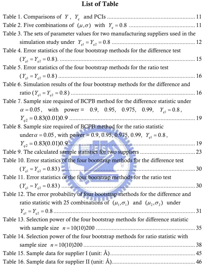
List of Table

Table 1. Comparisons of Y , Y_q and PCIs ... 11 Table 2. Five combinations of ( , )μ σ with Y =_q 0.8 ... 11 Table 3. The sets of parameter values for two manufacturing suppliers used in the

simulation study under Y_q1=Y_q2 =0.8... 12 Table 4. Error statistics of the four bootstrap methods for the difference test

(Y_q1 =Y_q2 =0.8). ... 15 Table 5. Error statistics of the four bootstrap methods for the ratio test

(Y_q1 =Y_q2 =0.8) ... 16 Table 6. Simulation results of the four bootstrap methods for the difference and

ratio (Y_q1 =Y_q2 =0.8) ... 16

Table 7. Sample size required of BCPB method for the difference statistic under α=0.05, with power = 0.9, 0.95, 0.975, 0.99, , ... 19 1 0.8 q Y = 2 0.83(0.01)0.9 q Y =

Table 8. Sample size required of BCPB method for the ratio statistic underα =0.05, with power = 0.9, 0.95, 0.975, 0.99, Y =_q1 0.8,

... 19

2 0.83(0.01)0.9

q Y =

Table 9. The calculated sample statistics for two suppliers ... 23 Table 10. Error statistics of the four bootstrap methods for the difference test

(Y_q1 =Y_q2 =0.83) ... 30 Table 11. Error statistics of the four bootstrap methods for the ratio test

(Y_q1 =Y_q2 =0.83) ... 30 Table 12. The error probability of four bootstrap methods for the difference and

ratio statistic with 25 combinations of ( , )μ σ_{1 1} and ( ,μ σ_{2 2}) under

... 31

1 2 0.8

q q

Y =Y =

Table 13. Selection power of the four bootstrap methods for difference statistic with sample size n =10(10)200... 35 Table 14. Selection power of the four bootstrap methods for ratio statistic with

sample size n =10(10)200... 38 Table 15. Sample data for supplier I (unit: Å)... 45 Table 16. Sample data for supplier II (unit: Å)... 46

List of Figure

Figure 1. Four processes with Y =_q 0.8... 12

Figure 2. Error probability of four bootstrap methods under Y_q2−Y_q1 =0 (Y_q1 =Y_q2 =0.8) ... 14

Figure 3. Error probability of four bootstrap methods under ( ) ... 14 1/ 2 1 q q Y Y = 1 2 0.8 q q Y =Y = Figure 4. The selection power of four bootstrap methods for the difference statistic with sample size n =10(10)200, Y =_q1 0.8, Y =_q2 0.9... 18

Figure 5. The selection power of four bootstrap methods for the ratio statistic with sample size n =10(10)200, Y =_q1 0.8, Y =_q2 0.9... 18

Figure 6. The sample size curve for the difference statistic under α =0.05, with power = 0.9, 0.95, 0.975, 0.99, Y =_q1 0.8, Y =_q2 0.83(0.01)0.9... 20

Figure 7. The sample size curve for the ratio statistic under α=0.05, with power = 0.9, 0.95, 0.975, 0.99, Y =_q1 0.8, Y =_q2 0.83(0.01)0.9... 20

Figure 8. An assembly drawing for the PDP products... 21

Figure 9. Histogram of data S1 ... 22

Figure 10. Histogram of data S2... 22

Figure 11. Normal probability plot for S1 ... 23

Figure 12. Normal probability plot for S2 ... 23

Figure 13. Error probability of four bootstrap methods under ( ) ... 29 2 1 0 q q Y −Y = 1 2 0.83 q q Y =Y = Figure 14. Error probability of four bootstrap methods under Y_q1/Y =_q2 1 (Y_q1 =Y_q2 =0.83) ... 29

Figure 15. The selection power for the difference statistic with sample size , , 10(10)200 n = Y =_q1 0.8 Y =_q2 0.81. ... 41

Figure 16. The selection power for the ratio statistic with sample size , , 10(10)200 n = Y =_q1 0.8 Y =_q2 0.81. ... 41

Figure 17. The selection power for the difference statistic with sample size , , 10(10)200 n = Y =_q1 0.8 Y =_q2 0.82... 41

Figure 18. The selection power for the ratio statistic with sample size , , 10(10)200 n = Y =_q1 0.8 Y =_q2 0.82... 41

Figure 19. The selection power for the difference statistic with sample size , , 10(10)200 n = Y =_q1 0.8 Y =_q2 0.83. ... 41

Figure 20. The selection power for the ratio statistic with sample size , , 10(10)200 n = Y =_q1 0.8 Y =_q2 0.83. ... 41

Figure 21. The selection power for the difference statistic with sample size , , 10(10)200 n = Y =_q1 0.8 Y =_q2 0.84... 42 Figure 22. The selection power for the ratio statistic with sample size

10(10)200

n = , Y =_q1 0.8, Y =_q2 0.84... 42 Figure 23. The selection power for the difference statistic with sample size

, ,

10(10)200

n = Y =_q1 0.8 Y =_q2 0.85. ... 42 Figure 24. The selection power for the ratio statistic with sample size

, ,

10(10)200

n = Y =_q1 0.8 Y =_q2 0.85. ... 42 Figure 25. The selection power for the difference statistic with sample size

, ,

10(10)200

n = Y =_q1 0.8 Y =_q2 0.86... 42 Figure 26. The selection power for the ratio statistic with sample size

, ,

10(10)200

n = Y =_q1 0.8 Y =_q2 0.86... 42 Figure 27. The selection power for the difference statistic with sample size

, ,

10(10)200

n = Y =_q1 0.8 Y =_q2 0.87... 43 Figure 28. The selection power for the ratio statistic with sample size

, ,

10(10)200

n = Y =_q1 0.8 Y =_q2 0.87... 43 Figure 29. The selection power for the difference statistic with sample size

, ,

10(10)200

n = Y =_q1 0.8 Y =_q2 0.88... 43 Figure 30. The selection power for the ratio statistic with sample size

, ,

10(10)200

n = Y =_q1 0.8 Y =_q2 0.88... 43 Figure 31. The selection power for the difference statistic with sample size

, ,

10(10)200

n = Y =_q1 0.8 Y =_q2 0.89... 43 Figure 32. The selection power for the ratio statistic with sample size

, ,

10(10)200

n = Y =_q1 0.8 Y =_q2 0.89... 43 Figure 33. The selection power for the difference statistic with sample size

, ,

10(10)200

n = Y =_q1 0.8 Y =_q2 0.9... 44 Figure 34. The selection power for the ratio statistic with sample size

, ,

10(10)200

Notations

T : target value

LSL : the lower specification limits preset by the process engineers USL : the upper specification limits preset by the process engineers

d : the half specification width

m : the midpoint between the upper and lower specification limits

μ : the population mean

σ : the population variation

2

σ : the population standard deviation

i

π : supplier i

n : the number of the sample size drawn from suppliers πi

B : the number of bootstrap resamples

N : simulation replicated times

* 1

ˆ

q

Y : the Yˆ_q1 of bootstrap resamples from supplier I

* 2

ˆ

q

Y : the Yˆ_q2 of bootstrap resamples from supplier II

θ : the difference or the ratio of two suppliers’Y_qindex ˆ

θ : the estimator of θ

*

ˆ

θ : the associated ordered bootstrap estimate of θ

* ˆ

θ : the sample average of the bootstrap estimates B

*

1. Introduction

Process capacity indices (PCIs) are used to determine whether a production process is capable of manufacturing items within a specified tolerance. The larger process capability index means the more capable process and reflects that the process output is closer to the target or the smaller process spread. Kane (1986) started that the quantification of the process mean and variation is central to understand the quality of units produced from a manufacturing process and PCIs can be used to measure process potential at the stage of the initial production setting. These facts bring the issue of supplier selection based on PCIs into the main focus. There are some assumptions when we use PCIs to measure the process performance. Ng and Tsui (1992) indicated that PCIs are designed to monitor the performance should be normal or near-normal processes with symmetric tolerance. In contrast with the assumption for using PCIs, the quality yield index is proposed to rectify this disadvantage. also emphasizes the ability of the process clustering around the target. According to these advantages, we use the quality yield index to distinguish which supplier has better process capability. Using the hypothesis test to find the larger . Unfortunately, statistical properties of comparing two estimated are mathematically intractable. In this paper, we apply the bootstrap resampling technique to obtain the lower confidence bound on the difference (ratio) of two estimated . Four types of bootstrap method, including the standard bootstrap (SB), the percentile bootstrap (PB), the biased corrected percentile bootstrap (BCPB), and the bootstrap-t (BT) method will be compared. Performance comparisons are made among these in terms of error probability and selection power. Through these comparisons, a better method would be selected to apply in supplier selection.

q Y q Y q Y q Y q Y q Y

This paper is organized as follows. We first give a review of PCIs and a brief introduction on the yield. We then take the connection between the process loss and the quality yield. In section 3, we compared two suppliers’ by the hypothesis testing and bootstrap method estimation technique will be applied. For selecting the best one of four bootstrap methods, we set the simulation layout in order to analyze the error probability and the selection power in section 4. For convenience of applications, we tabulate the sample size required for various designated selection power in section 5. Finally, we investigate a real-world case and apply the selection procedure using actual data collected from the factories to reach a decision in the supplier selection in section 6.

q

2. Literature Review

2.1. Process Capability Indices

Process capability indices are convenient and powerful tools for measuring process performance proposed by several researchers such as Boyles (1991), Pearn

(1992), Kushler and Hurley (1992), Kotz and Johnson (1993), Vännman and Kotz (1995), Vännman (1997), Kotz and Lovelace (1998), Pearn

.

et al

.

et al (1998), Pearn

and Shu (2003) and references therein. By taking into consideration process location, process variation, and manufacturing specifications, those indices quantify process performance and reflect process consistency, process accuracy, process yield, and process loss. The process indices C_p, C_pk, C_pm and C_pmk take natural process tolerance, manufacturing specifications, process centering, and the target value of the process into consideration and take advantage of unitless measures. Those indices convey critical information regarding whether a process is capable for reproducing items satisfying the customer’s requirement. In practice, a minimal capability requirement would be preset by the customers/engineers. If the prescribed minimum capability fails to be met, one would conclude that the process is incapable. The first process capacity index appearing in the literature was the precision index C_p and defined as (see Juran (1974) and Kane (1986)):

6 p USL LSL C σ − = ,

where is the upper specification limit, is the lower specification limit, and

USL LSL

σ is the process standard deviation. The index C_p measures process precision (process quality consistency) and does not consider whether the process is centered. In order to reflect the deviations of the process mean from the target value, the index

pk

C was proposed. It considers process variation and location of process mean which is defined as: min{ , } min , 3 3 3 pk pu pl d m USL LSL C C C μ μ μ σ σ σ − − − − ⎧ ⎫ = = _{⎨ ⎬}= ⎩ ⎭ ,

where μ is the process mean, d =(USL LSL)/2− , and m=(USL LSL /2+ ) . However, C_pk alone still cannot provide adequate measure of process centering. That is, a large C_pk does not really say anything about the location of the mean in the tolerance interval. To help account this, Hsiang and Taguchi (1985) introduced the index C_pm, which was also proposed independently by Chan (1988). The index is related to the idea of squared error loss, (where T is the target value), and this loss-based process capability index

. et al 2 ( ) ( ) loss X = X T− pm C , sometimes called Taguchi index. The index emphasizes on measuring the ability of the process to cluster around the target, which therefore reflects the degrees of the process targeting (centering). The index C_pm incorporates with the variation of production items with respect to the target value and the specification limits preset in the factory. The index

pm C is defined as: 2 2 6 ( pm USL LSL C T σ μ ) − = + − .

Pearn et al . (1992) proposed an index called C_pmk, which combines the merits of the before three basic indices C_p, C_pk and C_pm. The index C_pmk has been defined as:

{

}

(

)

2 2 min , 3 pmk USL LSL C T μ μ σ μ − − = + − .

The index C_pmk is more sensitive to the departure of the process mean μ from the target value T than the other three indices C_p, C_pk and C_pm.

Those indices are effective tools for process capability analysis and quality assurance. We could divide these indices into two categories according to the target value T. The first includes C_p and C_pk, which are independent of . Process loss incurred by the departure from the target is neglected. The second category includes

T

pm

C and C_pmk, which rectify the disadvantage by taking the target value into account. The limitation on using those indices requires the assumption that the quality characteristic measurement must be obtaining from normal distributions. Somerville and Montgomery (1996) presented an extensive study to illustrate how poorly the normally based capability indices perform as a predictor of process fallout when the process is non-normally distributed. If the normally based capability indices are still used to deal with non-normal process data, the value of the capacity indices are incorrect and might misrepresent the actually product quality. Although new capacity indices have been developed for non-normal distributions, those indices are harder to compute and interpret, and are sensitive to data peculiarities such as bimodality or truncation. Moreover, those indices do not explicitly account for the manufacturing cost or customer’s loss. Process quality yield index is proposed to remedy these

disadvantages. q

Y

2.2. Quality Yield Y_q and Relation Indices 2.2.1. Process Yield

Traditionally, process yield Y is defined as the percentage of the processed product units passing the inspections. Units are inspected according to specification limits placed on various key product characteristics and sorted into two categories: accepted (conforming items) and rejected (defectives). Process yield has long been the most common and standard criteria used in the manufacturing industries for judging process performance. For product units rejected during the inspection, additional costs would be incurred to the factory for scrapping or reworking. All passed product units are treated equally and accepted by the producer. No additional cost to the

factory is required. The definition of Y index is

( ) USL LSL

Y =

_∫

dF x ,

where and are the upper and the lower specification limits, respectively and

USL LSL

( )

F x is the cumulative distribution function of measured characteristic x . The

disadvantage of yield measure is that it does not distinguish the products that fall inside of the specification limits. Customers do notice unit-to-unit difference in these characteristics, especially if the variance is large and/or the mean is offset from the target.

2.2.2. Process Loss

To rectify this disadvantage, the quadratic loss function is considered to distinguish the products by increasing the penalty as departure from the target increases. However, the quadratic loss function itself does not provide comparison with the specification limits and depends on the unit of the characteristic. To address these issues, Johnson (1992) developed the relative expected loss for a symmetric

case as: e L

(

)

2 2 2 2 2 ( ) _{( )} e T x T L dF x d d σ μ ∞ −∞ + − ⎡ − ⎤ = _{⎢ ⎥} = ⎣ ⎦

∫

,

where _{σ is the process variance, μ is the process mean,} 2 _{T is the target value}

and is the half specification width. This measure has a direct relationship with ( d = USL LSL− )/2 pm C because _{(3 )} 2 e pm

L ₌ C − _{. The disadvantage of the index is}

the difficulty in setting a standard for the index since it increases from zero to infinity. e

L

2.2.3. Quality Yield Y_q

The main idea of the quality yield index is that it penalizes yield for the variation of the product characteristics from its target. Ng and Tsui (1992) suggested it by connecting the proportion-conforming-based index Y and loss-function-based index . Unlike the yield index , the quality yield focuses on the ability of the process to cluster around the target by taking the relative loss within the specifications into consideration. It is different from the expected relative worth index defined by Johnson by truncating the deviation outside the specifications. With this truncation, will be between zero and one and thus has better interpretation. Then the index defined as:

q Y e L Y Y_q q Y q Y 2 2 ( ) 1 USL q LSL x T Y d d ⎡ − ⎤ = _⎢ − _⎥ ⎣ ⎦

∫

F x . ( )

the proportion of “perfect” products. By relating to the yield measure, which is familiar to engineers, it is much easier for the engineers to understand and accept this capacity measure. The advantage of the index over the index is that the value of the former goes from zero to one. Similarly to the yield index, the Y measure, the ideal value of is one, which provides the user a clear concept about the standard. Similar to yield Y , the index does not rely on the normality assumption. And it can be interpreted as the average degree of products reaching ‘on target’. q Y L_e q Y q Y

In recent years, several methods have been proposed about . Pearn

(2004a) proposed a reliable approach for measuring by converting the estimate into a lower confidence bound for process with a very low fraction of defectives. And Pearn (2005) further applied a nonparametric but computer intensive method called bootstrap to obtain a lower confidence bound on for capability testing purposes. In this paper, we would use the quality index to judge which supplier has a better process performance.

q Y et al . q Y . et al q Y q Y

2.3. Investigation in Supplier Selection

The decision-maker usually faces the problem of selecting the best manufacturing supplier from several available manufacturing suppliers. There are many factors, such as quality, cost, and service and so on, that need to be considered in selecting the best supplier. Production quality is one of the key factors in supplier evaluation. For this reason, several selection rules have been proposed for selecting the means or variance in analysis of variance by Gibbons .et al (1977), Gupta and

Panchapakesan (1979), Gupta and Huang (1981) for more detail. Process capability indices are useful management tool, particularly in the manufacturing industry. Tseng and Wu (1991) considered the problem of selecting the best manufacturing process from available manufacturing processes based on the precision index k C_p and a modified likelihood ratio selection rule is proposed. Chou (1994) developed three one-sided tests (C_p, C_pu, C_pl ) for comparing two process capability indices in order to choose between competing process when the sample size are equal. Huang and Lee (1995) considered the supplier selection problem based on the index C_pm, and developed a mathematically complicated approximation method for selecting a subset of processes containing the best supplier from a given set of processes. Pearn (2004b) further provided useful information regarding the sample size regarding the sample size required for various designated selection power by using a simulation technique. A two-phase selection procedure was developed to select a better supplier and to examine the magnitude of the difference between the two suppliers. Chen and Chen (2004) offered four approximate confidence interval methods, one based on the statistical theory given in Boyles (1991) and three based on the bootstrap method, for selecting a better one of two suppliers. However, the method of comparing two suppliers in term of has not yet been discussed. In order to select a better supplier in process cabability, this article proposes the hypothesis testing for comparing the capability of two suppliers based on index.

. et al q Y q Y

3. Selection Method

3.1. Selecting a Better Supplier by Comparing Two Y_q Indices

Since we can not compare two suppliers directly, we have to sample some products made by two suppliers, and use some statistical analysis to compare which one has better process capability. Then we decide whether switch the present supplier or not. Let πi be the pollution assumed to be normally distributed with mean μi

and variance 2 i

σ , i =1,2, and are the independent random samples from

1, 2,..., _i

i i in

x x x

i

π , . In most applications, if a new supplier#2 (S2) wants to compete for the orders by claiming that its capability is better than the existing supplier#1 (S1), then the new S2 must furnish convincing information justifying the claim with a prescribed level of confidence. Thus, the supplier selection decision would be based on the hypothesis testing comparing the two values

1,2 i = q Y 0: q1 q 2 H Y ≥Y 1: q1 q 2 H Y <Y .

If the test rejects the null hypothesis H Y0 : q1 ≥Yq2 , then one has sufficient

information to conclude that the new S2 is superior to the original S1, and the decision of the replacement would be suggested. Equivalently, this test hypothesis problem can be rewritten as:

versus

0: q2 q1 0

H Y −Y ≤ H Y₁: _q2−Y_q1>0 (difference testing) versus (ratio testing).

0: q2/ q1 H Y Y ≤ 1 1 1 q 2 1 q i 1: q2/ q1 H Y Y >

Thus, if the lower confidence bound for the difference between two process capability indices is positive and then S2 has a better process capability than S1. Otherwise, we do not have sufficient information to conclude that the S2 has a better process capability than S1. In this case, we would believe that is true, i.e. . Similar, if the lower confidence bound between two process capability indices is great than 1, then S2 has a better process capability than S1. Otherwise, if the lower confidence bound of the ratio statistic is less than 1, and then we would conclude that S1 has a better process capability than S2.

2 q Y −Y 0: q2 q1 0 H Y −Y ≤ 1 q q Y ≥Y 2/ q Y Y

Based on above reasons mentioned, we should know the information about the point estimator of . Ng and Tsui (1992) proposed a sample estimator based on a finite population of products. Suppose q

Y

1, 2,...,

i i in

x x x denote the sample

measurements of product characteristics. It follows that are estimated by collected sample data and can be defined as follows: q

2 2 1 ( ) / ˆ i q LSL Xi USL X T d Y n < < ⎡ − − ⎤ = _{⎢ ⎥} ⎣ ⎦

∑

.

It is important to find a lower bound on the rather than just the sample point estimate. The index can be rewritten as follows (see Pearn q

Y q Y et al (2004a)): .

( )

2 2 ( ) USL q _LSL e x T Y Y dF x Y L d ⎡ − ⎤ = − _{⎢ ⎥} ≥ − ⎣ ⎦

∫

.

Thus, the measure provides a lower bound on the . We can obtain the lower 100γ% confidence bound on by calculating the lower 100

e

Y L− Y_q

q

Y γ₁% confidence

bound on Y and the upper 100γ2% confidence bound on Le (γ γ γ= × ). Pearn 1 2

(2004a) obtain the 100γ% lower confidence bound for and simultaneously can be expressed as:

. et al Y_q Y

(

)

(

)

₂

₍

₎

2 ˆ ˆ 2 3 1, 2 3 1 ˆ 1 ; L q L e n n P Y C Y C L x λ φ φ γ γ λ ⎛ ⎡ ₊ ⎤ ⎞ ⎜ _{≥ − ≥ − −}⎢ ⎥ ⎟ ⎜ ⎢_⎣ ′ − ⎥_⎦ ⎟ ⎝ ⎠ ≥ , where CL is the 100γ% lower bounds for Cpk, is sample size, n

2

2 ˆ

(1 ; )

n

x′ −γ λ is the (lower) (1−γ₂)th percentile of the 2

( )

n x′ λ distribution

(

)

2 2 ˆ _/ n n x T S λ₌ ⎡ ₋ ⎤ ⎣ ⎦ ( 1 / n i i x =

∑

₌ x n, S_n =

∑

_in₌₁⎡_⎣

(

x_i−x

)

2/n⎤_⎦1/2) and

(

)

2 2 1 1 ˆ n e i i L x nd = =

∑

−T .

However, their investigations are all developed for evaluating whether a single supplier’s process conforms to a customer’s requirements. Due to the complexities of the sampling distributions of Yˆ_q2 −Yˆq1 or , constructions of exact

confidence intervals for and are difficult. 2 ˆ q Y /Yˆq1 2 ˆ q Y −Yˆq1 Yˆq2 /Yˆq1 3.2. Bootstrap Methodology

The bootstrap is the idea that in the absence of any other knowledge about a population, the distribution of values found in a random sample of size from the population is the best guide to the distribution in the population, introduced by Efron (1979, 1982). Franklin and Wasserman (1991) proposed an initial study of three bootstrap methods for obtaining confidence intervals for

n

pk

C when the process was normally distributed. Franklin and Wasserman (1992) also proposed an initial study of these bootstrap lower limits for C_p, C_pk , and C_pm. Chen and Tong (2003) obtained the C_pk1−C_pk2 confidence interval using bootstrap methods under a normal distribution of observation. We can find most of them concluded that the

performance such bootstrap limits for PCIs is quite satisfactory in the majority of these cases. It can be applied whenever the construction of confidence intervals for parameters using the standard statistical techniques becomes intractable. The simulation results performed in the bootstrap confidence limits were as well as the lower confidence limits applied by the parametric method in the normal process environment. Without using distribution frequency tables to compute approximate probability values, the bootstrap method generates a unique sampling distribution based on the actual sample rather than the analytic methods.

In the following four bootstrap confidence limits are employed to determine the lower confidence bounds of difference and ratio statistics and the results are used to select the better supplier of the two selections. For n₁=n₂ = , let two bootstrap n

samples of size n drawn with replacement from two original samples be denoted by

{

* * *

} {

* * *

}

11, 12,..., 1n 21, 22,..., 2

x x x x x x _n . The bootstrap sample statistics , and

are computed. There are possibly a total of such samples, the statistic is calculated for each of these, and the resulting empirical distribution is referred to as the bootstrap distribution of the statistic. Due to the overwhelming computation time, it is not of practical interest to choose such samples. Eforn and Tibshirani (1986) indicated that a roughly minimum of 1,000 bootstrap resamples is usually sufficient to compute reasonably accurate confidence interval estimates for population parameters. For accuracy purpose, we consider

* 1 ˆ q Y * 2 ˆ q Y _nn n n 3,000 B = bootstrap resamples (rather than 1,000). Thus, we take B =3,000 bootstrap estimates

* * 2 ˆ ˆ q Y θ = * 1 ˆ _q Y − of θ =(Y_q2 −Y_q1) * * 2 ˆ ˆ q Y θ = * 1 ˆ / Y_q of θ =(Yq2/ Yq1),

respectively and then ordered from smallest to the largest where =1,2,…..,l B

( )* *2 ˆ ₍ˆ q l Y θ = * 1 ( ) ˆ )_{q l} Y − _{( )}* * 2 ˆ ˆ or θ_l =(Y_q * 1 ( ) ˆ /Y_q )_l .

Four kinds of bootstrap confidence intervals can be derived, including the standard bootstrap confidence interval (SB), the percentile bootstrap confidence interval (PB), the biased corrected percentile bootstrap confidence interval (BCPB), and the bootstrap-t (BT) method introduced by Efron (1981) and Efron and Tibshiraniwill (1986) are conducted in this paper. The generic notations ˆ θ and _θˆ* _{will be used}

to denote the estimator of θ and the associated ordered bootstrap estimate. Construction of a two-sided 100(1 2 )%− α confidence limit will be described. We note that a lower 100(1−α)% confidence limit can be obtained by using only the lower limit. The formulation details for the four types of confidence intervals are displayed as follows.

[A] Standard Bootstrap (SB) Method

From the bootstrap estimates B ˆ_{( )}* l

θ , l =1,2,..., ,B the sample average and the sample standard deviation can be obtained as:

* 1 ˆ B θ = _{( )}* 1 ˆ B l l θ =

∑

, 1/ 2 2 * * ( ) 1 1 _{ˆ ˆ} 1 B l l S B θ θ θ = * ⎡ _{⎡ ⎤} ⎤ =_{⎢ ⎢} − _{⎥ ⎥} ⎣ ⎦ − ⎣

∑

⎦ . The quantity _S*

θ is an estimator of the standard deviation of ˆθ is approximately

normal. Thus, the 100(1 2 )%− α SB confidence interval for θ can be constructed as:

[θˆ*−z S_{α θ}* , θˆ*+z S_{α θ}*],

where ˆθ is the estimated θ for the original sample, and z_α is the upper α quantile of the standard of the standard normal distribution.

[B] Percentile Bootstrap (PB) Method

From the ordered collection of ˆ_{( )}* l

θ , l =1,2,..., ,B the α percentage and 1− percentage points are used to obtained the α 100(1 2 )%− α PB confidence interval for θ

[θˆ_{( )}*_αB , θˆ₍*_(1−α)B)]. [C] Biased-Corrected Percentile Bootstrap (BCPB) Method

While the percentile confidence interval is intuitively appealing it is possible that due to sampling errors, the bootstrap distribution may be biased. In other words, it is possible that bootstrap distribution may be shifted higher or lower than would be expected. A three steps procedure is suggested to correct for the possible bias by Efron (1982). First, we use procedure the ordered distribution of _θˆ* _{and calculate}

the probability _p0=_P(θˆ* _≤θ 0

ˆ ) . Second, we compute the inverse of the cumulative distribution function of a standard normal based upon p₀ as z0 =φ( )p0 ,

0

(2 )

L

p =φ z −zα pU =φ(2z0+zα). Finally, by executing these steps we obtain the 100(1 2 )%− α BCPB confidence interval [ ˆ₍* ₎ L p B θ , ˆ₍* U ) P B θ ]. [D] Bootstrap-t (BT) Method

By using bootstrapping to approximate the distribution of a statistic of the form

ˆ

ˆ

(θ θ− )/S_θ, the bootstrap approximation in this case is obtained by taking bootstrap samples from the original data values, calculating the corresponding estimates _θˆ*

T =(_θˆ*_{- ˆθ )/ . The hope is then that the generated distribution will mimic the}

distribution of T. The 10

S

0(1 2 )%− α BT confidence interval for θ may constitute as: [θˆ*−t Sα* θ*ˆ , * * ˆ ˆ _{t S} α θ* θ − ], where _t*

α and t1*−α are the upper α and 1− quantiles of the bootstrap α

t-distribution respectively, i.e. by finding the values that satisfy the two equation P((θˆ*- ˆθ ) /S_θ*>t_α*)= and P((α θˆ*- ˆθ ) /S_θ*>t₁*_−α)= − 1 α

4. Performance Comparisons of Four Bootstrap Methods

4.1. Simulation Layout Setting

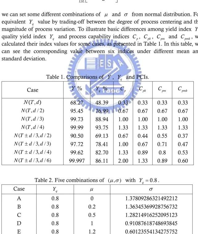
We consider mainly two characteristics of importance in the capacity of a process, the process location relative to its specification limits and the process spread. The more capable is the process reveals the closer the process output is to the mid-point of specification limits and the smaller the process spread. Based on the relationship 2 2 ( ) 1 ( USL q LSL X T Y d d ⎡ − ⎤ = _⎢ − _⎥ ⎣ ⎦

∫

F x , )

we can set some different combinations of μ and σ from normal distribution. For equivalent value by trading-off between the degree of process centering and the magnitude of process variation. To illustrate basic differences among yield index , quality yield index and process capability indices

q

Y

Y

q

Y C_p, C_pk, C_pm and C_pmk, we

calculated their index values for some cases, as presented in Table 1. In this table, we can see the corresponding value between six indices under different mean and standard deviation.

Table 1. Comparisons of Y , Y_q and PCIs.

Case Y % Yq % Cp Cpk Cpm Cpmk ( , ) N T d 68.27 48.39 0.33 0.33 0.33 0.33 ) 2 / , (T d N 95.45 76.99 0.67 0.67 0.67 0.67 ) 3 / , (T d N 99.73 88.94 1.00 1.00 1.00 1.00 ) 4 / , (T d N 99.99 93.75 1.33 1.33 1.33 1.33 ) 2 / , 3 / (T d d N ± 90.50 69.13 0.67 0.44 0.55 0.37 ) 3 / , 3 / (T d d N ± 97.72 78.41 1.00 0.67 0.71 0.47 ) 4 / , 3 / (T d d N ± 99.62 82.70 1.33 0.89 0.8 0.53 ) 6 / , 3 / (T d d N ± 99.997 86.11 2.00 1.33 0.89 0.60

Table 2. Five combinations of ( , )μ σ with Y_q = 0.8.

Case Yq μ σ A 0.8 0 1.37809286321492212 B 0.8 0.2 1.36345369928756732 C 0.8 0.5 1.28214916252095123 D 0.8 1 0.91087618748693845 E 0.8 1.2 0.60123554134275752

Figure 1. Five processes with Y_q = 0.8.

Table 3. The sets of parameter values for two manufacturing suppliers used in the simulation study under Y_q1 =Y_q2 =0.8.

Component Y_q1 Case Y_q2 Case

1 0.8 A 0.8 A 2 0.8 A 0.8 B 3 0.8 A 0.8 C 4 0.8 A 0.8 D 5 0.8 A 0.8 E 6 0.8 B 0.8 A 7 0.8 B 0.8 B 8 0.8 B 0.8 C 9 0.8 B 0.8 D 10 0.8 B 0.8 E 11 0.8 C 0.8 A 12 0.8 C 0.8 B 13 0.8 C 0.8 C 14 0.8 C 0.8 D 15 0.8 C 0.8 E 16 0.8 D 0.8 A 17 0.8 D 0.8 B 18 0.8 D 0.8 C 19 0.8 D 0.8 D 20 0.8 D 0.8 E 21 0.8 E 0.8 A 22 0.8 E 0.8 B 23 0.8 E 0.8 C 24 0.8 E 0.8 D 25 0.8 E 0.8 E

We set five processes with different combinations of ( , )μ σ with in Table 2. The distribution of these combinations of

0.8 q

Y =

( , )μ σ is showed in Figure 1. These five processes are equivalent according to and all have 80% average degree of products reaching ‘perfect’ or ‘on target’. Hence, we performed a series of simulations to investigate the error probability and selection power of difference and ratio testing statistics for the performance comparisons of four bootstrap methods in order to make a comparative study among bootstrap confidence limits. We selected twenty-five values for two manufacturing supplier used in the simulation study given in Table 3. By this way, we cloud test the bootstrap methods’ performance in different conditions. (i.e. ‘on-target’ and ‘off-target’ range). For each combination, 3000 random samples were generated and the corresponding bootstrap confidence intervals were showed for each of these samples later.

q

Y

4.2. Error Probability Analysis

The error probability is the proportion of times that we wrongly reject the null hypothesis H Y₀: _q1 ≥Y_{q 2}, while actually H Y₀: _q1≥Y_{q 2} is true. For the test, we will calculate the proportion of times the LCB of Y_q2 −Y_q1 is positive and the LCB of

is larger than 1. A sample of size

2/ q

Y Y_q1 n =100 was drawn with

bootstrap resamples, and the single simulation was then replicated times. Figures 2 and 3 show the error probability of those four bootstrap methods for the difference and ratio statistics with 25 combinations (it also called 25 cases in the following) tabulated in Table 3, respectively. Usually, the reasonable probability of error selection is less than a maximum value

3,000

B =

3,000

N =

*

α -condition. The frequency of error selection is a binomial random variable with N =3,000 and . Then we can calculate a 99% confidence interval for error probability is

* _0.05 α = * * * 0.05 (1 )/ 0.05 2.576 (0.05 0.95)/3000 0.05 0.0103 Z N α ± × α −α = ± × × = ± .

That is, if we set , the reasonable interval would be the range from 0.0397 to 0.0610.

* _0.05

α =

Before we selected the parameter of the error test, we tried many different combinations of N , B and . Because too low value of n N would make the

random error significant and the tendency between different cases wouldn’t be obvious. On the other hand, too high value of N will make the 99% confidence bound too narrow. Cases were out of interval easily in this condition and it was difficult to judge which bootstrap method was better. As the result, we tested many combinations of the parameter and finally selected N =3,000, , and

to perform the error test. Considering different value of may also affect the layout of the error curve for four bootstrap methods, different values of were also simulated under the same combination (

3,000 B = 100 n = Y_q q Y 3,000 N = , B =3,000, ) and then we found that the tendency of the curves were more significant by the increase of value in . And the relative location between the curve of four methods wasn’t changed. Based on these tests, we finally selected the case of with

100 n = q Y 0.8 q Y =

3,000

N = , , and to perform the error test in four bootstrap

methods. 3,000 B = n =100

difference error

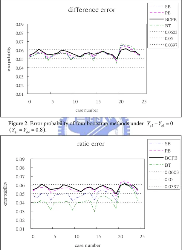
0.01 0.02 0.03 0.04 0.05 0.06 0.07 0.08 0.09 0 5 10 15 20 25 case number erro r pro ba bi lit y SB PB BCPB BT 0.0603 0.05 0.0397

Figure 2. Error probability of four bootstrap methods under Y_q2 −Y_q1 =0

(Y_q1=Y_q2 =0.8). ratio error 0.01 0.02 0.03 0.04 0.05 0.06 0.07 0.08 0.09 0 5 10 15 20 25 case number erro r p ra b il it y SB PB BCPB BT 0.0603 0.05 0.0397

Figure 3. Error probability of four bootstrap methods under Y_q2/Y =_q1 1

After the difference statistic, there were three occurrences out of the 25 cases were outside the interval (0.0397, 0.0603) for the SB method. And for the PB method, there were three occurrences beyond these limits. Only two occurrences were outside the interval for the BCPB method, and there were three occurrences beyond these limits for the BT method. As for the ratio test, there were 3 occurrences out of the 25 cases outside the interval (0.0397, 0.0603) for the SB, PB and BCPB methods. The most cases out of the limits were for the BT method (7 occurrences). We could find that the PB, SB and BCPB methods had similar number of occurrences outside the interval for the 25 cases and the BT method had the least cases out of the upper bound in the ratio test.

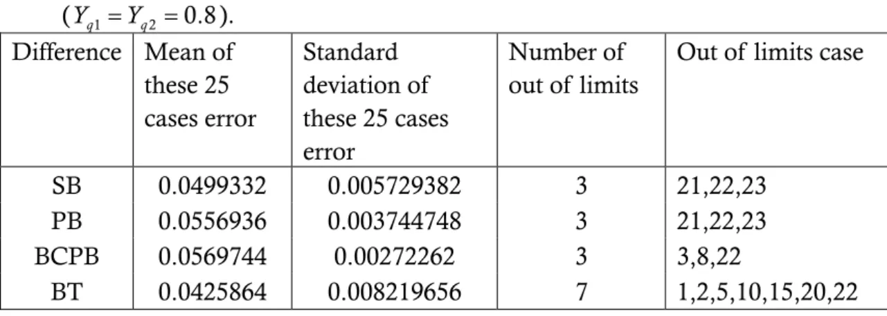
By the following Tables 4-5, we can further examine the mean and standard deviation of the error probability for four methods. We could find that the mean of the error probability for the BCPB method was the farthest from the target and the standard deviation was the lowest compared with the other methods in the different test. In the ratio test, the mean for the BT method was the farthest from the setting 0.05 and the standard deviation was the highest in four bootstrap methods. And The BCPB method still had the lowest standard deviation. The SB method has the closest mean to the target, but its deviation was higher than the PB and BCPB methods in Table 5. In the two tests, we could find that the BCPB method had a higher mean of error probability in four methods but it could keep a lowest standard deviation in all four methods. We also performed the error test in Y_q1 =Y_q2 =0.83 (see Tables 10-11 and Figures 11-12 in Appendix A) and found that as the value became larger, the standard deviation of the error probability for four methods got larger. In this condition, the BCPB method still had the smallest variation among four bootstrap methods. Considering the application in high quality measuring, the BCPB method could keep the steadiest value of the error probability.

q

Y

Table 4. Error statistics of the four bootstrap methods for the difference test (Y_q1 =Y_q2 =0.8). Difference Mean of these 25 cases error Standard deviation of these 25 cases error Number of out of limits

Out of limits case

SB 0.0552528 0.004475521 3 21,22,23

PB 0.0556936 0.003744748 3 21,22,23

BCPB 0.0567064 0.002709163 2 3,22

Table 5. Error statistics of the four bootstrap methods for the ratio test (Y_q1 =Y_q2 =0.8). Difference Mean of these 25 cases error Standard deviation of these 25 cases error Number of out of limits

Out of limits case

SB 0.0499332 0.005729382 3 21,22,23

PB 0.0556936 0.003744748 3 21,22,23

BCPB 0.0569744 0.00272262 3 3,8,22

BT 0.0425864 0.00821965 6 7 1,2,5,10,15,20,22

Table 6. Simulation results of the four bootstrap methods for the difference and ratio (Y_q1=Y_q2 =0.8).

Difference statistic Ratio statistic

1 q

Y case Y_q2 case Bootstrap

methods _Error prob. Average LCB Standard deviation of LCB Error prob. Average LCB Standard deviation of LCB 0.8 E 0.8 E SB PB BCPB BT 0.05267 0.05367 0.05467 0.05167 -0.03888 -0.03891 -0.03892 -0.03883 0.02429 0.02438 0.02449 0.02420 0.04900 0.05367 0.05500 0.04167 0.95201 0.95277 0.95277 0.95088 0.02905 0.02930 0.02947 0.02876 0.8 C 0.8 C SB PB BCPB BT 0.05433 0.05533 0.05600 0.05400 -0.05799 -0.05800 -0.05807 -0.05790 0.03621 0.03635 0.03649 0.03610 0.05033 0.05533 0.05633 0.04133 0.92872 0.93050 0.93042 0.92622 0.04241 0.04302 0.04329 0.04171 0.8 A 0.8 E SB PB BCPB BT 0.05000 0.05133 0.05467 0.04767 -0.04986 -0.04927 -0.04858 -0.05043 0.02917 0.02924 0.02928 0.02910 0.04200 0.05133 0.05467 0.03100 0.93888 0.94146 0.94227 0.93560 0.03355 0.03413 0.03426 0.03285 0.8 A 0.8 A SB PB BCPB BT 0.05200 0.05300 0.05433 0.05167 -0.05843 -0.05850 -0.05851 -0.05834 0.03598 0.03608 0.03624 0.03590 0.04767 0.05300 0.05467 0.03933 0.92819 0.92991 0.92990 0.92567 0.04212 0.04270 0.04298 0.04147 0.8 A 0.8 C SB PB BCPB BT 0.05633 0.05700 0.06100 0.05700 -0.05822 -0.05827 -0.05829 -0.05816 0.03624 0.03637 0.03656 0.03611 0.05033 0.05700 0.06100 0.04233 0.92845 0.93021 0.93019 0.92589 0.04243 0.04304 0.04337 0.04172

In addition, we calculated an average lower bound and the standard deviation of the lower bound based on the N =3000, B =3000, n =100 difference trials. Table 6 also displays the average lower confidence bound (LCB) and standard deviation of the LCB for each of the four bootstrap confidence intervals and we tabulated these values of 25 cases for four bootstrap methods in Table 12 in Appendix A. In the Figures 2-3, and Table 6, we could find the different cases’ influence on the error probability. The average and standard deviation of LCB was significantly different between these cases. By setting different cases and comparing the performance of four methods, a suitable bootstrap method could be selected. In Tables 4-5, we found the performance of the BT method was the worst. It couldn’t keep steady error probability in different cases. The SB, PB, and BCPB methods had similar performance in two tests, but the BCPB method had the smallest variation and the least out of limit cases.

4.3. Selection Power Analysis

In this stage, we further compared the performance of those four bootstrap methods. Different simulations of selections of selection power analysis were conducted with sample sizes n =10(10)200 for Y =_q1 0.8 , . Because the difference between four methods in 25 cases didn’t change too much, we could set two on-target (

2 0.83(0.01)0.9 q

Y = T

μ = ) cases to compare selection power in four methods. The selection power is the probability of rejecting the null hypothesis H Y₀: _q1≥Y_{q 2} while actually H Y₁: _q1 <Y_{q 2} is true. Under our setting, the selection power is the proportion of times that the LCB of Y_q2−Y_q1 is positive for the difference statistic. And for the ratio statistic, the selection power is the proportion of times that the LCB of was larger than 1 in the simulation. Figures 4-5 display the power of four Bootstrap methods for the difference and ratio statistic with 2

/ q

Y Y_q1

10(10)200

n = , ,

, respectively and other simulation values and corresponding figures are displayed in Tables 13-14 and Figures 15-34 in Appendix B.

1 0.8 q Y = 2 0.9 q Y =

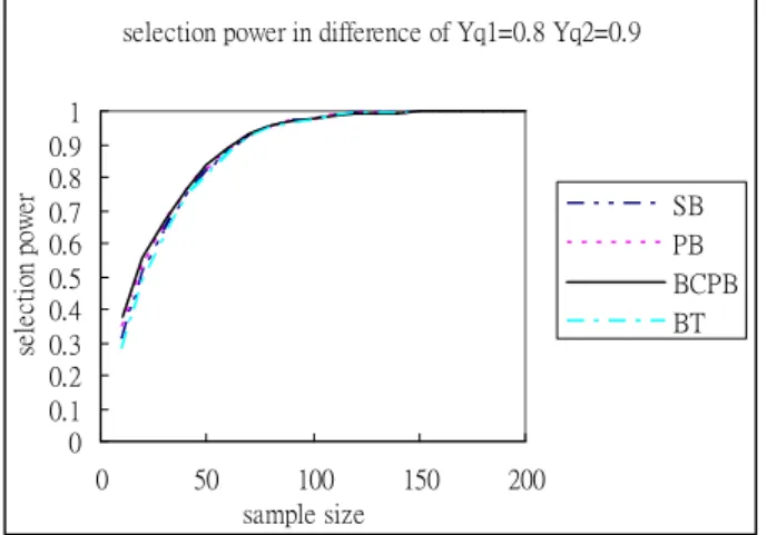
According to Figures 4-5, we found that the difference test has similar power between four cases. For ratio test, the PB and BCPB methods had smaller required sample size with fixed selection power. In the other, the SB and BT methods had larger required sample size with fixed selection power. In terms of error probability analysis above and selection power analysis, the BCPB and PB methods had more correct error probability and better selection power with fixed sample size, but the BCPB method was better than the PB method in some considerations. Therefore, we recommend that the best of those four bootstrap methods in our approach was the BCPB method.

selection power in difference of Yq1=0.8 Yq2=0.9 0 0.1 0.2 0.3 0.4 0.5 0.6 0.7 0.8 0.9 1 0 50 100 150 200 sample size se le ct ion pow er SB PB BCPB BT

selection power in ratio of Yq1=0.8 Yq2=0.9

0 0.1 0.2 0.3 0.4 0.5 0.6 0.7 0.8 0.9 1 0 50 100 150 200 sample size se le ctio n po w er SB PB BCPB BT

Figure 4. The selection power of four bootstrap methods for the difference

statistic with sample size ,

, . n =10(10)200

1 0.8 q

Y = Y =_q2 0.9

Figure 5. The selection power of four bootstrap methods for the ratio statistic with sample size n =10(10)200, Y =_q1 0.8,

2 0.9 q

5. Supplier Selection Based on BCPB Method

5.1. Sample Size Determination with Designated Selection Power

In practice, if a new supplier (S2) wants to convince customers their capability is better than the existing supplier (S1). Credible information should be proposed with a prescribed level of confidence. Thus, we must determine the sample size to collect actual data from the factories for designated selection power. By the last stage, we investigated the BCPB method with B =3,000 bootstrap resamples, and the

times were replicated. The selection power is computing the proportion of rejecting the null hypothesis

3,000

N =

0: q1 q2

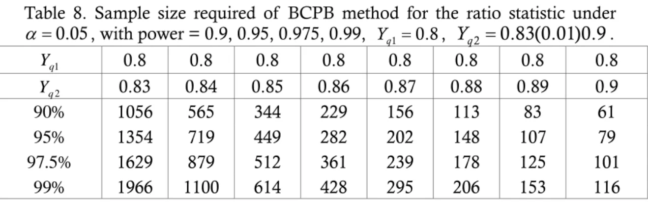
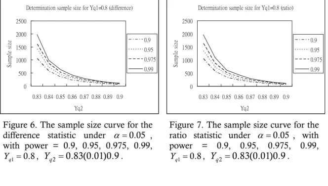
H Y ≥Y while actually H Y₁: _q1<Y_q2 is true. For users’ convenience in applying our procedure in practice, we tabulated the sample size required of the BCPB for various designated selection power = 0.90, 0.95, 0.975, 0.99 and the difference with Y =_q1 0.8 and Y =_q2 0.83(0.01)0.9 in Table 7 (the ratio in Table 8). From Tables 7-8, it could be find the smaller the sample size required for the fixed selection when the larger the value of difference δ =Y_q2−Y_q1 between two suppliers. By this phenomenon, if we want to recognize the smaller of the difference and have larger designated selection power, the more collected sample is required to account the smaller uncertainty in estimation. Figures 6-7 show the curve of the sample size based on Tables 7-8, and we could observe the tendency of curves between two tests with four kinds of power value is similar.

Table 7. Sample size required of BCPB method for the difference statistic under 0.05 α= , with power = 0.9, 0.95, 0.975, 0.99, Y =_q1 0.8, Y =_q2 0.83(0.01)0.9. 1 q Y 0.8 0.8 0.8 0.8 0.8 0.8 0.8 0.8 2 q Y 0.83 0.84 0.85 0.86 0.87 0.88 0.89 0.9 % 90 1050 571 350 232 159 112 82 63 % 95 1425 720 441 301 204 145 103 81 % 5 . 97 1613 863 520 351 240 177 126 93 % 99 1974 992 635 425 288 208 153 118

Table 8. Sample size required of BCPB method for the ratio statistic under 0.05 α= , with power = 0.9, 0.95, 0.975, 0.99, Y =_q1 0.8, Y =_q2 0.83(0.01)0.9. 1 q Y 0.8 0.8 0.8 0.8 0.8 0.8 0.8 0.8 2 q Y 0.83 0.84 0.85 0.86 0.87 0.88 0.89 0.9 % 90 1056 565 344 229 156 113 83 61 % 95 1354 719 449 282 202 148 107 79 % 5 . 97 1629 879 512 361 239 178 125 101 % 99 1966 1100 614 428 295 206 153 116

Determination sample size for Yq1=0.8 (difference) 0 500 1000 1500 2000 2500 0.83 0.84 0.85 0.86 0.87 0.88 0.89 0.9 Yq2 S am p le s ize 0.9 0.95 0.975 0.99

Determination sample size for Yq1=0.8 (ratio)

0 500 1000 1500 2000 2500 0.83 0.84 0.85 0.86 0.87 0.88 0.89 0.9 Yq2 S am p le s ize 0.9 0.95 0.975 0.99

Figure 6. The sample size curve for the difference statistic under α =0.05 , with power = 0.9, 0.95, 0.975, 0.99,

, .

1 0.8 q

Y = Y =_q2 0.83(0.01)0.9

Figure 7. The sample size curve for the ratio statistic under α =0.05 , with power = 0.9, 0.95, 0.975, 0.99,

1 0.8 q

Y = , Y =_q2 0.83(0.01)0.9.

5.2. Selecting the Better Supplier

By Tables 7-8 in 5.1, in order to make users do this selection work conveniently, we develop the practical step-by-step procedure for practitioners to use in making supplier selection decisions. The main steps in tests could be done in the following : 1. Determine the minimum requirement of Y_q values for two candidates and the minimum difference.

2. Based on the BCPB method, Obtain the sample size required with selection power.

3. Apply Kolmogorov-Smirnov test to affirm whether the sample data of two suppliers is normal distributed.

4. If the LCB of Yˆ_q2 −Yˆ_q1 is positive or the LCB of Yˆ_q2 /Y is greater than 1, then ˆ_q1

we conclude that the S2 is better than the S1. Otherwise, since we don’t have sufficient information to reject the null hypothesis H Y₀: _q1≥Y_q2, we would believe that the S1 has better capacity than the new S2.

6. Application Example: PDP Producer with

ITO Glass Supplier Selection

Plasma Display Panel (PDP) is a new display technology which can be used to produce high-screen TV. PDP allows displays to be thinner and less weight than Cathode Ray Tube (CRT). Compared with other displays, it also has large viewing angles and can’t be effect by the magnetic field. With these advantages, PDP technology can accord with the demand for science and consumer electronics industries in the future.

The basic operation principle of PDP is similar to CRT and the fluorescent lamp. PDP screen is composed of a lot of light space, every little space call a cell. The operation principle of every cell is similar to the fluorescent lamp. Like a small volume of the fluorescent lamp, it has the gas of helium (He), neon (Ne), xenon (Xe). When the high-tension electricity is passed, it will release the electric energy and touch off the gas in cell to discharge the gas emitting the ultraviolet ray. Utilizing the ultraviolet ray to stimulate the red, green and blue phosphorescence on the coating glass, three kinds of primary colors will be produced. By controlling the ultraviolet ray in different intensity through different cells, it can produce various combinations of three primary colors and different kinds of colors are made.

In the following Figure 8, the manufacturing procedure of PDP is composed of two mainly parts. One is close to users called front process including glass substrate, transparent electrode, bus-electrode and dielectric layer. Another one is rear process. Among them include color phosphor, barrier rib, address electrode and glass substrate. The producer combines the two processes then the control circuit is inserted in the middle. In this process, it needs accurate line in two substrates and do well matching with the control circuit to ensure it couldn’t be problematic in bringing the light. Through some treatment and inspecting the stability, a basic PDP screen has been finished. Figure 8 is taken from http://digital.photosharp.com.tw/digital.

In PDP producing process, transparent electrode is made by etching Indium Tin Oxide (ITO) glass substrate. The thickness of ITO membrane has a critical influence in the resistance value and it is very important for the manufacturing procedure of PDP. So the accuracy of ITO membrane in thickness plays a very important role in product yield. PDP manufacturers usually look for a supplier to obtain ITO glass substrate. By these reasons, it is a very important thing for PDP manufacturer to find a good ITO glass substrate supplier.

We already know that the thickness of ITO membrane is an important quality characteristic. To illustrate how to select a better process capability between two suppliers, we presented a PDP manufacturer which is located in Taiwan. The manufacturer wanted to select a better ITO glass substrate supplier between two glass manufacturers. For a particular model of the PDP investigated, the upper specification limit (USL) of ITO membrane thickness is set to USL 1500 Å; the lower specification limit (LSL) of membrane thickness is set to Å, and the target value of membrane thickness is set to

= 1100

LSL =

1300

T = Å.

6.1. Data Analysis and Supplier Selection

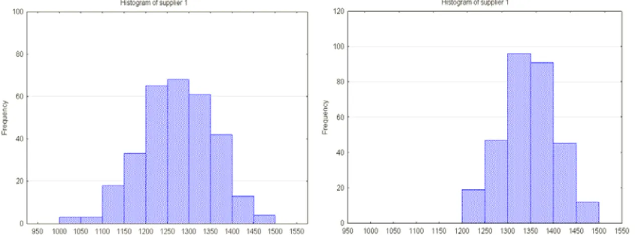
For the step1 of supplier selection, the practitioner should input the minimum requirement of and the minimum difference for two candidates. And in the step2, we decided the sample size based on the minimum requirement, the minimum difference and the selection power we need. In this application, the upper specification limit was 1500 Å, the lower specification limit was 1100 Å and the target value was 1300 Å. The minimum requirement for ITO product was 0.8 and the minimum difference of is 0.06 between two candidates with selection power 0.95. By checking the preset table (Tables 7-8) with the data, we had to take 301 samples for the difference statistics and 282 samples for the ratio statistics. In the case, we took 310 samples for S1 and S2 respectively.

q

Y

q

Y