A sliding-mode approach to fuzzy control design

IEEE TRANSACTIONS ON CONTROL SYSTEMS TECHNOLOGY, VOL. 4, NO. 2, MARCH 1996 141

A

Sliding-Mode Approach to

Fuzzy

Control Design

J.

C.

Wu and T.

S. Liu,

Member, IEEE

Abstract- This study develops a method for fuzzy control design with sliding modes in which robustness is inherent. Fuzzy control is formulated to become a class of variable structure system (VSS) control. Sliding modes are used to determine best values for parameters in fuzzy control rules, thereby robustness in fuzzy control can be improved. A switching manifold is prescribed and the phase trajectory is demanded to satisfy both the reaching condition and the sliding condition for sliding modes. Both computer simulations and experiments are carried out for an apparatus which can to some extent represent cornering motion of a motorcycle on which a rider leans to maintain stability. Experimental results demonstrate that the proposed method outperforms both proportional integral derivative (PID) control and neural-network-based fuzzy control.

I. INTRODUCTION

UZZY control is a direct method for controlling a system

F

without the need of a mathematical model, in contrast to the classical control which

is^

an indirect method with a mathematical model. Fuzzy control has been implemented in many industrial applications. There are, however, few systematic procedures available for analysis and design of fuzzy control. In this study, a fuzzy control design with sliding mode is proposed to improve control system performance. The sliding mode is used to determine parameters in fuzzy control rules, in which the robustness is inherent in variable structure systems (VSS’s) with sliding modes. With the aid of sliding modes, it provides an effective design method of fuzzy control to ensure robustness. To validate the proposed method, an experimental apparatus is designed and conducted in which an inverted pendulum is hinged to a rotating disk. Both computer simulations and experiments are carried out. This apparatus is designed in such a way that it can, to some extent, represent the cornering motion of a motorcycle on which a rider leans to maintain stability.

Fuzzy control research based on the fuzzy set theory [29] was initiated by Mamdani 1191. Braae and Rutherford [2] proposed both an algebraic model and a linguistic model for fuzzy control. The algebraic model cannot deal directly with the rules of a fuzzy controller. This limitation of the algebraic model led to the linguistic model that provided a

linguistic structure for dealing with fuzzy control. Tang and Mulholland [27] compared fuzzy control with proportional integral derivative (PID) control. Langari [ 151 proposed an analytical formulation of fuzzy control which is essentially nonlinear. Kawaji et al. [ 141 proposed to design fuzzy control

Manuscript received May 12, 1995. Recommended by Associate Editor, J .

Winkelman. This work was supported in part by the National Science Council. Taiwan, ROC under Grant NSC83-0401-E009-081.

The authors are with the Department of Mechanical Engineering, National Chiao Tung University, Hsinchu 30050, Taiwan, ROC.

Publisher Item Identifier S 1063-6536(96)02073-8.

employing the knowledge of a proportional derivative (PD) control, in which the fuzzy control is treated as PD control with gain switching. Lin and Kung [17] proposed a fuzzy- sliding mode controller (FSC) that improves VSS control with the aid of fuzzy control. The FSC is based on the VSS control theory and entails the advantages of VSS control and fuzzy control. In contrast to Lin and Kung who improved VSS control with the aid of fuzzy control, the current study aims to determine the parameters in fuzzy control rules based on sliding modes to ensure robustness. Kawaji and Matsunaga 1131 proposed a method of generating fuzzy rules for servo- motors based on the VSS control. They determine linguistic values in fuzzy control rules and choose the best linguistic value based on both experience and trial and error. By contrast, in this study the switching manifold is treated as a reference model, and parameters in fuzzy control rules are determined to satisfy both reaching and sliding conditions using sliding-mode theory.

In this study, fuzzy control is designed with sliding modes that are basic motions in a VSS. The VSS with sliding modes was proposed and elaborated upon by Emelyanov [4] and Itkis [12]. The VSS control is generally modeled in the phase space. It employs switching and discontinuous control actions to drive a phase trajectory toward a prescribed hyperplane and to force the phase trajectory to slide on the hyperplane. Robustness is an important feature of VSS control. A detailed survey can be found in [\11]. For discrete- time VSS control, only quasi-sliding modes are achieved in practice due to the limitation of sampling rates [20]. Sira-Ramirez [25] investigated stability conditions and the convergence for discrete-time sliding-mode control systems. Furuta [7] presented a discrete sliding-mode control based on discrete Lyapunov functions. He also presented discrete- type VSS control [8] and its application to self-tuning control. Pieper and Goheen [23] achieved quasi-sliding modes in a discrete input-output model with nonminimum phase. Padeh and Tomizuka 1221 proposed a discrete-time VSS control for a direct-drive robot.

In this study, Section I1 describes definitions and assump- tions and then formulates fuzzy control. In Section 111, sliding- mode theory is described. Fuzzy control rules are enacted with the aid of sliding modes in Section IV. Section V describes a case study to validate the proposed method.

11. FUZZY CONTROL A. DeJinitions and Assumptions

are described in the following.

Several assumptions that facilitate formulation in this study

142 IEEE TRANSACTIONS ON CONTROL SYSTEMS TECHNOLOGY, VOL. 4, NO. 2, MARCH 1996

Fig. 1. Membership functions of input variables

Assumption 1: Let X be a universe. P and N are fuzzy

subsets whose membership functions are continuous but not differentiable mappings ,U:

X

-+ [0, 11. Define p.p(z) and P f i ( 4 as

P f i ( 4 = 1 - P p ( 4 (2)

where

xu

and 21 denote the upper and lower bounds in the

universe, respectively.

P

and N are shown in Fig. 1, in which they form fuzzy partitions of a closed, bounded region. Both

P

and N are normal, i.e., sup, p p ( z ) = sup, p # ( z ) = 1,

IL' E [zl,

z,].

Moreover, for each z E [ZL, z,]

(3) CLp(4

+

P.rv(.) = 1.

Assumption 2: Let A = {A,} and

B

= { B l ) be collections of fuzzy subsets over E and EC, respectively. E and EC denote the bounded universe for scaled error e and scaled error change ec. This study assumes that each of

2

and B

contains only two fuzzy subsets as described in Assumption 1. According to ( 3 ) , for any e E E and ec E EG

2 2

PCLA,k) = PLBl(ec) = 1. (4)

3=1 1=1

Assumption 3: Let U be a bounded universe for scaled

control action U . Fuzzy rules

R,

defined on

E

x EC x U , are expressed as the union (U) of four individual rules

R

=

U

R,,l. ( 5 )

3 , l

Fuzzy rules [26] containing two input variables can be written as a simple form

R,,z:IfeisA, andecisB1 ,thenu,,t = p i +p",+piec e E E , e c E EC, u,,~ E U , i = 1

>

. . . 4

,

(6) where p t , p: , and p i denote parameters of a linear dependence between nonfuzzy values of input variables and control action. The fuzzy controller contains four rules, since only two fuzzy subsets, P and N , are defined for each of

E

and EC as described in Assumption 2.

B.

Formulation

Fuzzy sets provide a useful foundation to handle human knowledge pertaining to a real world problem and contribute to the notation of fuzzy control. The formulation for fuzzy control is described in the following: Given crisp input values eo and eco, assume that input values can be treated as fuzzy singletons Eo and Eo, i.e.,

1, if e = eo 0, otherwise

/la,(e) = (7)

and similar condition holds for E O . Denote f,, 1 as a mapping from E x EC to U , U,,[ = f,,l(e, ec) as described in (6). Since Eo and

EO

are fuzzy singletons, ba_sed on the extension principle [ 3 ] one can define fuzzy sets

C,

in

U

as

1

C, are also fuzzy singletons, as shown in (8). From ( 5 ) and (6), fuzzy rules

R

can be written as

R =

@

[FAJ ( e )

0

P E L (e.) @ Pet

(.)I

(9)

,,1

where @ denotes the union operator and

0

the algebraic product operator. In this study, the algebraic product instead of the minimum operator is employed and results in interactivity among elements in (9). The fuzzy set of control action U, in terms of input values eo, eco, and fuzzy rules R, can be written as

PZL(U) = [P.;, (e> @ P&) (eel1 O

R

=

@

{ P i , (eo)

0

P& (eco) 0 PE, ( U ) > (10) ,,I

where o denotes a composition operator. Let w3, z = p i

(eo)@

p ~ ~ ( e c 0 ) denote rule strength of (6). The center of gravity method is employed for defuzzification, and the crisp value U , can be written as

,>1

Since

cj,

wj, 1 = 1 from (4), (1 1) becomes

Since both

w,,

1 and U,, 1 in (12) are continuous functions of eo and eco, U , is a continuous and nonlinear function of eo and eco, i.e., fuzzy control is essentially a class of nonlinear control.

To gain insight into the relationship between fuzzy control and VSS control, the phase plane of E and EC can be divided

WU AND LIU: SLIDING-MODE APPROACH

I

XR

XP

lT7

VII

into nine regions

as

depicted in

Fig.

2(a) which accounts for

I1

m

T 7 TTT

e

Ix

Region I: Region 11: Region 111: Region IV: Region V: Region VI: Region VII: Region VIII: Region IX:

This study assumes XP = -2 and x f i = 2. Equation (12) can be written as in Region I in Region 11 in Region I11 in Region IV in Region V in Region VI in Region VI1 in Region VI11 in Region IX (1 3 ) where

H.O.T.

denotes higher-order terms and

D,,

E,,

and

F,,

and m = 1,

.

. .

,

9 denotes parameters that are functions of p ; , z = I , . .

.

,

4 , j = 0, I, 2 . Specifically 3 3 3 1 1 1

D1

= P o

El

= P I Fl = p , 0 3 = P o

E3 =PI

F3

= p 2 0 7 = P i E7

'P:

F7

= P ; D9 = P i E9 =p:. Fcj = p ; . (14)

ec=

e c =

143

e c

e=+

I

e=xm

ec=xR

ec=xp

FL

e=xp

I

e=xR

(b) Fig. 2.

Determination of control actions based on partition planes.

(a) Nine partition planes of error (e) and error change (ec). (b)

The 12 parameters p i can be determined based on conditions in sliding modes. Each of f,, m = 1 , . . .

,

9 is a continuous and differentiable function in terms of

eo

and eco. U,, however, is continuous but not differentiable on lines e = xp, e = x f i ,

ec = x p , and ec = x f i . Control actions uo in these nine regions are shown in Fig. 2(b), in which FL and F N L denote linear and nonlinear functions, respectively. Control actions due to Regions I, 111, VII, and IX are linear functions since u J , ~ in (6) are linear functions, and only one rule fires in each of these four regions. Hence, fuzzy control is similar to

PD control in these four regions. Fuzzy control in essence resembles VSS control since control actions U , change with divided regions on the phase plane as shown in (13). Therefore, fuzzy control can be treated as a class of VSS control. Besides, the lines e = xp, e = x f i , ec = x p , and ec = X N that divide the phase plane can be regarded as switching lines.

144 IEEE TRANSACTIONS ON CONTROL SYSTEMS TECHNOLOGY, VOL. 4, NO 2, MARCH 1996

There are, however, two differences between fuzzy control and VSS control. First, a VSS control is generally devised with a sliding mode, whereas fuzzy control is not. Second, control actions of VSS control often discontinuously change whenever the trajectory crosses switching lines, on which sliding modes occur. By contrast, the variation of control action U , in (13) for fuzzy control is continuous, and no sliding mode occurs on four switching lines.

To implement conventional fuzzy rules, an input space has to be divided into many fuzzy subsets, and the consequences of fuzzy conditional propositions are also fuzzy subsets. This study employs fuzzy rules proposed by Takagi and Sugeno

[26] to reduce the number of fuzzy subsets and rules. The consequences of rules represent linear input-output relations of a system. By adjusting crisp values p i in (6), via sliding modes in the current study, fuzzy rules can effectively correlate fuzzy subsets so that a multivariable and complex system is tractable. Although in this study each input variable contains merely two fuzzy subsets, the control inputs are nonlinear functions f ( e , ec) as shown in (13). The consequences of conventional fuzzy rules are fuzzy subsets that are specified. The center positions of these fuzzy subsets act like single

&

in (6). In contrast to consequences in conventional fuzzy rules, crisp u3,1 defined in (6) depends on p: and p i in addition to

p i .

Besides, unlike conventional fuzzy rules, ug,l varies with both e and ec. This is equivalent to the division of input spaces in the conventional method. Hence, this approach is comparable to conventional fuzzy rules, in which seven or more subsets are often employed on each universe. The present method can indeed reduce the need of so many fuzzy sets and rules. Nevertheless, the limitation of this approach is that the consequences as expressed in (6) are not fuzzy, and thus a great deal of theories in fuzzy logic cannot be directly applied.

111. SLIDING MODE THEORY

A VSS can be treated as a combination of subsystems, each with a fixed structure and each operating in a specified region of phase space. VSS control is a class of nonlinear control whose control actions are discontinuous. To implement VSS control, switching functions have to be selected. The dynamic behavior of the system is dominated by the switching functions. Due to discontinuous control actions, sliding modes occur whenever the trajectory on the phase plane crosses switching manifolds. When the system motion is constrained on the switching manifolds, the motion is said to be in the slid- ing mode. Consider an nth-order control system represented

by the state equation

X = A(x)

+

B(x)u

where x denotes state vector and U input vector. Generally,

the transient dynamics of VSS consists of two conditions: a reaching condition and a sliding condition. Under the reaching condition, the desired response aims to reach the switching manifold in finite time. The switching manifold S is written as

where s denotes a switching function. Parameters of the switching manifold dominate the dynamic behavior of the system during sliding mode control. The Lyapunov function approach is one of methods for specifying reaching condition. To avoid the chattering that is present in VSS control, one can smooth out the control discontinuity by defining a bound- ary layer of thickness Cp. Accordingly, denote the Lyapunov function candidate

V(x) = $(s -

ay.

₍₁₅₎

The reaching condition is obtained by differentiating (15) with respect to time, i.e.,

V ( x ) = (s - @ ) ( S -

6)

<

0 when (s -

@)

#

0. ₍₁₆₎ The control law for the reaching condition is written as

. = { U ' when s(x)

>

0

U- when s(x)

<

0

where U+ and U- denote different control actions. This control

law, which is discontinuous on s = 0, is given according to prescribed switching function s such that the switching manifold can be reached in finite time. Hence, the VSS control entails different control actions on either side of the given switching manifold.

Under a sliding condition, the trajectory asymptotically goes to the origin of the phase plane. The dynamics can be formulated as S(x) = 0; that is a necessary but not sufficient condition for the state trajectory to remain on the switching manifold. Solution of i(x) = 0 gives the equivalent control ueq. The feature of VSS control is that the sliding mode occurs on the switching manifold, and the system remains insensitive to external disturbances and plant uncertainty. The sliding- mode theory entails switching functions that are represented by lines on the phase plane. The phase plane facilitates the qualitative analysis. VSS control is generally devised with sliding-mode theory. It can also be devised without a sliding mode, but such a system would not possess the associated merits.

For discrete-time system, only quasi-sliding modes can be accomplished. Replacing derivative terms in (16) by forward difference terms yields

[ ~ ( k

+

1) - @ ( k

+

1) - ~ ( k )

+

@ ( k ) ] [ s ( k ) - @ ( k ) ]

<

0. (17)

This condition is a necessary but not sufficient condition for the existence of quasi-sliding modes. The inequality equation ~ 4 1

Is(k

+

1) - @ ( k

+

1)1

<

Is(k) - @ ( k ) ( (18) is a sufficient condition for quasi-sliding modes that guarantees the convergence of state trajectories. Equation (18) can be decomposed into two inequality equations, i.e.,

[ s ( k

+

1) - @ ( k

+

1) - s ( k )

+

@ ( k ) ] [ s ( k

+

1) - @ ( k

+

1)

+

s ( k ) - @ ( k ) ] . Sign [ s ( k ) - @ ( k ) ]

<

0 . Sign [ s ( k ) - @ ( k ) ]

>

0. (19) (20)

s

= {XI s(x) = O}

WU AND LIU: SLIDING-MODE APPROACH 145

It is noted that (19) is equivalent to (17). In addition, (18) is equivalent to [7]

[ s ( k

+

1) - @ ( k

+

1)12

<

[ s ( k ) -

@@)I2.

IV. SLIDING MODES FOR FUZZY RULES

This study employs a linguistic system [2] to design fuzzy control, for which sliding modes are used to determine param- eters in control rules. Consider a linguistic system with the representation in discrete time

x”(k

+

1) = A/’[x”(k), U”] ₍₂₁₎

where k denotes the time step, x”(k) the linguistic state vector, U” a linguistic input, and A”(.) a linguistic map

whose parameters are linguistic values. Linguistic variables rely on the user’s linguistic values such as “positive” and “negative,” and are described in terms of fuzzy subsets as shown in Assumption 2 of Section

11-A.

The linguistic system enables modeling fuzzy control as a nonlinear system. Assume x”(k

+

1) contains two terms and U” only one term, i.e., a

second-order system and single input (21) can be written as x:’(k

+

1)

=xP(k)

x/2/(k

+

1) = A”[x?(k), z $ ( k ) , ~ ” ( k ) ] . (22) Let xd be the setpoint and linguistic error e ” ( k ) =

xy(k

+

1) - Z d , then (22) becomes

ec”(k)

=xy(k

+

1) -

xy(k)

xy(k

+

2 ) = A”[e/’(k), ec”(k), u”(k)] (23)

Fig. 3. Switching function s and phase point

4

on a phase plane.

(14). In addition, control actions in these four regions are linear functions that facilitate the determination of parameters. Control actions in the four regions can be written as

U =

o;wc

(26)

where 0; =

[D,

F,],

T = 1, 3, 7 , 9, and w,’ =

[1 ec]. Due to (14), O,, consists of elements p i . The switching function is defined as s = Xe

+

ec shown in Fig. 3 where

x

is a positive constant. It is seen that the switching function is located in the second and fourth quadrants. This function can be treated as a phase trajectory of Pd(e, ec). Furthermore, for ease of sensor feedback, e and ec instead of s are employed. Under the reaching condition, from (23) the manifold s ( k

+

1) = 0 can be treated as a reference model

E,

e

where ec” denotes linguistic error change. The linguistic _{? ( k}

+

_{2) = XR;(k)}

+

xd

₍₂₇₎

where XR = 1/(x

+

1). Since is a positive constant, XR is less than one. Hence, the reference model is stable. From (25)-(27)

system is investigated on the phase plane to combine with sliding mode. Treating A ” ( . ) as a rule set [lo], (23) thus becomes

xy‘k

+

2 ) =

A”

o [e”(k) x ec”(k) x u”(k)] where o denotes the composition operator and x the Cartesian product. The control action of a fuzzy controller is given by

U” = F g ( e , ec)

z ( k

+

2 ) = A”(e/’, ec”, O:,wc)

-

-

xd

(28) where

z

=

x”

-

9. For the reaching condition, it is desired to determine

O,,

such that z + 0 as k + 00. The VSS control with sliding mode can hence be considered as a model-reaching control, where the model reached in finite approach is implemented to specify the control action to obtain (24)

where Fg denotes a linguistic map. Equation (23), combined _{time represents the sliding equation, The Lyapunov function} with (24), becomes

2 - i 0 with the time step k as small as possible. Accordingly,

from (25) and (26), rewrite (19) and (20) as (25)

d l ( k

+

2) = A”[e’/, ec”, F g ( e , e c ) ] .

The design procedure is to first specify the response Pd(e, ec) on the phase plane and then design a fuzzy controller (24) to achieve this response. To carry out fuzzy control design, the control action is formulated, such as (13) on

the partition plane. Finally, the values of 12 parameters p ; , i = 1,

. . .

,

4, j = 0, 1, 2 are determined such that both desired reaching and sliding conditions can be satisfied to ensure robustness. To determine these values, Regions I, 111, VII, and IX are considered, since D,, E,, and F,, T = 1, 3 , 7 , 9 are equal to 12 parameters p i as shown in

[A”(e”, ec”,

o:wc)

-

xd

- e ( k )

-

XRec(k)

-

[A”(e”, ec”,

oLw,)

-

xd

+

X&e(k)

+

XRec(k) -

a.21

.

Sign [ s ( k ) - @ ( k ) ]

<

0

.

Sign [ s ( k ) - @(k)]

>

O

(29) (30) where

Xk

= ( x - l ) / ( x + l ) , @I = [ @ ( k + l ) - @ ( k ) ] / ( x + l ) , and @ 2 = [ @ ( k

+

1)

+

@ ( k ) ] / ( X

+

1). Inequalities (29) and

(30) are used to determine O,,, T = 3 when s ( k ) - @ ( k )

>

0, whereas O,,, T = 7 when s ( k ) - @ ( k )

<

0.

I46 IEEE TRANSACTIONS ON CONTROL SYSTEMS TECHNOLOGY, VOL. 4, NO. 2, MARCH 1996

Under the sliding condition, s ( k

+

1) - s ( k ) = 0 [7] is

required for the phase trajectory to remain on the switching manifold s ( k

+

1) = 0. Furthermore, using (23), s ( k

+

1) -

s ( k ) = 0 can be rewritten to become a reference model (3 1) Since both e and ec are scaled by gains, s = 0 represents a line passing the origin and Regions I, V, and IX as shown in Fig. 3. Moreover,

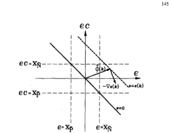
e,,,

T = 1, and 9 can be determined by (25), (26), and (31). This is similar to the procedure leading to the equivalent control ueq as described in Section 111. Nevertheless, from the above method one can find solutions of

O,,,

T = 1, 3,

7,

and 9 to satisfy both the reaching and sliding conditions. To further choose the best value of

e,,,

the slope X ( k ) of phase point

$(k)

at time step k is employed where X ( k ) is given by

? ( k

+

2) =

q k )

+

X&c(k)

+

Zd.

Since gradient V s ( k ) = [ X ( k )

11

and phase point & k ) =

[ e ( k ) ec(k)lT, (32) can be written as (Vs,

4)

= 0 where

(.,

.) denotes the inner product. Accordingly,

6

represents the null space of Vs. The function s = s ( k ) at time step

k

represents a line parallel to the line s = 0, whereas

- V s ( k )

denotes the flow direction of the phase point as shown in Fig. 3. X ( k ) is negative in the first and third quadrants but positive in the second and fourth quadrants. It is desired that X ( k ) is approaching

x

with not only k but also the overshoot as small as possible. This reasoning is similar to that in characterizing a transient response due to unit step input.

V. CASE STUDY

A. System Model

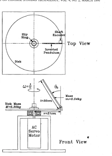
A rider-motorcycle integrated system can be treated as a man-machine system. Although a motorcycle is statically unstable in nature, appropriate steering by the rider can stabi- lize the motorcycle during riding. To maintain stability, with respect to tire bottoms on the ground, the moment arising from the gravity force must be equal to, but opposite to, the direction of the moment due to the centrifugal force during cornering. Forouhar [5] proposed a feedback control scheme based on robust optimal control theory to improve the dynamic behavior of motorcycles. Liu and Wu [ 181 employed the fuzzy control method to investigate the performance of

rider-motorcycle systems. In this study, an inverted pendulum hinged to a rotating disk as shown in Fig. 4 is used to represent cornering motion of a motorcycle on which a rider leans to maintain stability. This apparatus is designed in such a way that it can, to some extent, represent motion control involving the leaning angle of the rider’s body (represented by the inverted pendulum) and the banking speed of the motorcycle (represented by the disk). In a manner similar to the balance during motorcycle cornering, the inverted pendulum is not stable at any tilt angle unless both moments caused by the pendulum weight and the centrifugal force counteract each other. The inverted pendulum representing a rider’s body in

!

\\U

Disk Mass

_8..

‘=‘*-\A

M=6.30ko Servo Motor

View

Mass m=O.Olkg B

Front

View

Fig. 4. Schematic diagram of an inverted pendulum hinged to a rotating disk.

leaning morion is hinged to the rim of the rotating disk. The centrifugal force resulting from the rotating motion of the disk enables the inverted pendulum to rotate about the tangential direction of the disk. Rotating speeds of the disk that correspond to riding speeds of the motorcycle dominate the leaning motion of the inverted pendulum that corresponds to the rider’s leaning motion. This study regulates the tilting inverted pendulum to target angles using fuzzy control with sliding mode, in which target angles are prescribed to change during excursion and control input is the rotating speed of the disk. It is desired to vary rotating speeds, so that the tilt angle can be regulated by the centrifugal force that arises from disk rotation.

The Hamiltonian formulation constructs the system model in terms of generalized coordinates and generalized momenta and thus results in a set of first-order equations of motion. Furthermore, solution trajectories for equations of motion derived by the Hamiltonian formulation form a phase space which lends itself to the description of the qualitative behavior of the system. To derive Hamilton’s equations, generalized coordinates and generalized momenta are defined as

r

WU AND LIU: SLIDING-MODE APPROACH 147

0.02

-

0.01

.12

-0.02

0

3.14

6.28

Fig. 5 . Phase planes of 8 b and P O , without control.

Hamilton's equations [9] are accordingly written as

(34) where U denotes the generalized force, i.e., the torques of motor, COb and CO are damping coefficients of the inverted pendulum and the disk to account for viscous damping at joints, and

~b =

mi2

I ,

=

M r 2

+

m ( ~ - 1

.

sin 8b)'

IC = ml(r - $ 1 . sin O b ) cos 0 b .

Neglecting generalized force and damping, i.e., U = 0 and

cob

= CO = 0, (34) gives equilibrium points: p = 0, o b = 0,

&7r, f27r,

. .

-, whereas

Q

is arbitrary. If damping exists, as

depicted in Fig. 5, equilibrium points ( T , O), (3n, 0), etc., become stable nodes which account for the pendulum in the vertically downward direction.

B. Simulation Results

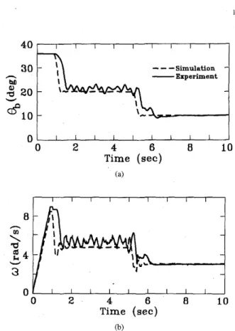
In this study, initial conditions are prescribed as: the angle of inverted pendulum 0 b = 36', the angular velocity of inverted

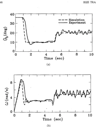
pendulum 0 b = 0, and the angular velocity of motor w = 0. The inverted pendulum is initially supported by a vertical strut such that 0 b cannot be larger than 36". Two cases are investigated in which the target angle change occurs at the fifth second. The target angle of the inverted pendulum in Case I is 20" from the start to the fifth second and 10" from

-

-

-Simulation h -Experiment M

0

2 4

6

8

10

Time (sec)

(a) 8 h

5

rd k 4

3

W

0

0

2

4 6 8 10

Time (sec)

(b) Fig. 6.

the inverted pendulum and (b) angular velocity of the motor in Case I. Simulation and experimental results of (a) angular displacement for

the fifth second to the end. The target angle of the inverted pendulum in Case I1 is 10' in _the former period-md 20" in the latter period. Since positive ( P ) and negative ( N ) are denoted as fuzzy subsets for input variables as depicted in Fig. 1, four fuzzy rules can be written, as in the form of (6)

where error e ( k ) denotes the current angle of the inverted pendulum minus the target angle and error change e c ( k ) the current error minus the error at the previous sampling time. In the above four rules, 12 parameters p i in the consequence are determined by sliding-mode theory as described in Section IV. Dashed curves in Figs. 6 and 7 show simulation results for Cases I and 11, respectively. It is seen that to track the larger target angle 20", it requires a larger motor angular velocity w . This applies to motorcycle cornering in the sense that only in a larger body lean of the rider can faster cornering motion be accomplished. The same control rules but different gains are used for both cases. The phase trajectories shown

148 IEEE TRANSACTIONS ON CONTROL SYSTEMS TECHNOLOGY, VOL. 4, NO. 2 , MARCH 1996 I I I I I I I I

- -

-

Simulation

-

Experiment - I I I I I I I I I 0 2 4 6 8 10 Time ( s e c ) (b) Fig. 7.

the inverted pendulum and (b) angular velocity of the motor in Case II. Simulation and experimental results of (a) angular displacement for

in Fig. 8 initiate from 8 b = 36" and ec = Oo, and

x

that denotes the slope of switching lines is the same in both cases. No chattering phenomenon occurs on switching lines since boundary layers are employed in (18). As shown in Fig. 8, the phase trajectories approach two switching lines but do not stay on them. This is anticipated since the switching lines are the prescribed reference lines and the control input for fuzzy control is continuous, as shown in Section 11; thus the sliding condition cannot be fulfilled perfectly. Besides, discrete-time VSS control can only achieve quasi-sliding modes according to [20].

C. Experimental Results

The schematic diagram of the experimental setup is shown in Fig. 9. A shaft encoder at the hinge of the inverted pen- dulum measures the tilt angle. An interface card transmits the position count to the PC to carry out the fuzzy control. The

sampling time of a PC command is 1 ms. A motor driver receives control signals via the interface card and enables instantaneous rotation motion of the AC servo motor. The initial angle of pendulum 0 b is 36" and the rotational velocity

of the motor w = 0.

Solid curves in Figs. 6 and 7 depict experimental results for variations of

O b

in two cases. Data is collected at a sample rate of 50 Hz. Experimental curves lag behind simulation curves, since in the experimental setup there exist mechanical and electrical time constants that are not accounted for in simulations. In contrast to simulation results, curve wiggle is present due to gear collision at backlash in the gear box

0

I I I

Switching

50

-100

L

0

10

20

30

40

(b)

Fig. 8. Simulation results of phase trajectories for (a) Case I and (b) Case I1

for the servo motor. The collision occurs whenever the motor undergoes large acceleration or deceleration. The collision

hence belongs to unknown nonlinearity. Since motor angular velocities w increase with target angles, the degree of collision increases with target angles. Furthermore, since variations of w increase with target angles as shown in Figs. 6(b) and 7(b), the wiggle of the O b curve also increases with target angles

as shown in Figs. 6(a) and 7(a). Fig. 10 shows Bode plots of

o b versus motor angular velocity w in both cases. The phase lag in Case I1 is larger than that in Case I. It is noted that compensating for larger phase lag requires more control effort. From the viewpoint of a rider-motorcycle system undergoing rider's posture change, Fig. 10 demonstrates that it takes more control effort for a rider to increase than to decrease the leaning angle.

WU AND LIU: SLIDING-MODE APPROACH 149 Interface Card haft ncoder Interface Card Count er Motor Driver

I

K

p

c

-80486 n

Fig. 11 compares the experimental results between the pro- posed method and PID control for target angles 20' and 10". Three gains for the PID controller are determined by Ziegler-Nichols tuning [6]. Dealing with the current system in the presence of nonlinearity, the proposed method outperforms

I-\ - 40 - I I I I

-

1 5 -

I I 1 1 1 1 1 1 1 1 I 1 1 1 1 1 1 1 I I 1 1 1 1 1 1

a

W

-

0 - 1 5

-

Ld

-

m Case I Case I1 E - 3 0 -

---

-

-45.

' I l f 1 1 1 ' 1 I I ' 1 1 1 ' 1 1 ' 1 ' ' ' I l l - n lo 0 0

2

2 4 6 8 10 Time( sec) (a) *O

...

Fuzzy control PID control 10 0 ' I I I I 0 2 4 6 8 10 Time(sec) (b) Fig. 11.

posed method and PID control.

Experimental results of the angular displacements using the pro-

PID control that yields significant angular variation. This is attributed to fuzzy control in essence exerting different control input among different phase plane regions as shown in (1 3). Control input for different regions is adjusted by the parameters of rules in this work.

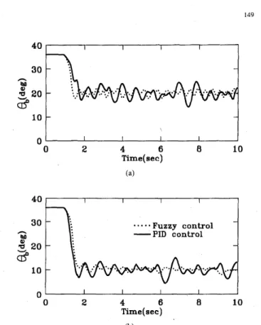
In the literature, there exist other fuzzy control meth- ods available, e.g., neural-network-based fuzzy control and adaptive fuzzy control. Fig. 12 compares experimental re- sults between the proposed method and neural-network-based fuzzy control 1161. In neural-network-based fuzzy control, a backpropagation algorithm is employed to learn membership functions and parameters in fuzzy rules. The backpropagation network consists of two nodes in the input layer, three hidden layers with ten nodes in each, and one node in the output layer. Input signals contain error e and error change ec, and the output signal is the motor angular velocity

w.

It is shown in Fig. 12 that the proposed method is comparable to neural-network-based fuzzy control. Due to the backpropaga- tion algorithm, however, neural-network-based fuzzy control spends about 250 times the CPU time for the proposed method, as depicted in Table I. Three disadvantages of the algorithm lead to long learning time. First, initial weighting values have to be randomly prescribed which result in slow convergence. Second, a set of sufficient input-output data has to be available for learning. Third, the algorithm often leads to unsatisfactory local minima of cost functions. Taking advantage of adaptive control, adaptive fuzzy control [ 11, [28] incorporates a training

algorithm which adjusts the parameters of fuzzy control based on input-output data. Its parameter adaption, however, only works well in dealing with uncertainties in terms of constant

150 IEEE TRANSACTIONS ON CONTROL SYSTEMS TECHNOLOGY, VOL. 4, NO. 2, MARCH 1996 30

I-

\

-

I

\

I

l o t

1

01 I I I I 0 2

4

6 8 10 Time( sec) (a) I I I I I

VSS-based fuzzy control NN-based fuzzy control

30 h M

4

20

a

10 I I I I

I

0 2

4

6 8 10 Time( sec) Fig. 12.

method and neural-network-based fuzzy control.

Experimental results of angular displacements using the proposed

TABLE I

CPU TIME COMPERSSION

The Present Method Neural-Network-Based Fuzzy Control

I

or slowly varying parameters versus VSS in nonlinearity and uncertainties in terms of quickly varying parameters. Fur- thermore, indirect adaptive fuzzy control [21] has to identify models using input-output data.

VI. CONCLUSIONS

This study proposes a method for fuzzy control design with sliding modes. Fuzzy control has been formulated to become a class of VSS control. Sliding modes facilitate determining the best values for parameters in fuzzy control rules. The Lyapunov function and the boundary layer have been employed to satisfy the reaching condition and to avoid chattering, respectively. In addition to computer simulations, experiments have been conducted to validate the proposed method.

In

comparison, the present method outperforms not only PID control but also neural-network-based fuzzy control. The success of the present method lies in the fact that fuzzy control inherently resembles VSS control, since both control actions vary with divided regions on phase planes.

It is difficult, however, to carry out the present method for very high-order systems with multi-input, for which an effective scheme would be required to enable state trajectories approaching sliding modes.

REFERENCES

C. Batur and V. Kasparian, “Adaptive expert control,” Int. J. Contr.,

vol. 54, no. 4, pp. 867-881, 1991.

M. Braae and D. A. Rutherford, “Theoretical and linguistic aspects of the fuzzy logic controller,” Automatica, vol. 15, pp. 553-577, 1979. D. Dubois and H. Prade, Fuzz)) Sets and Systems: Theory and Applica-

tions. New York Academic, 1980.

S. V. Emelyanov, Variable Structure Control Systems. Moscow: Nauka, 1967.

F. A. Forouhar, “Robust stabilization of high speed oscillations in single track vehicles by feedback control of gyroscopic moments of crankshaft and engine inertia,” Ph.D. dissertation, Univ. California, Berkeley, 1992. G. F. Franklin, J. D. Powell, and A. Emami-Naeini, Feedback Control

of Dynamic Systems, 3rd ed.

K. Furuta, “Sliding mode control of a discrete system,” Syst. Contr.

Lett., vol. 14, pp. 145-152, 1990.

-, “VSS-type self-tuning control-@ equivalent control approach,” in Proc. Amer. Contr. Con$, San Francisco, CA, 1993, pp. 980-984. H. Goldstein, Classical Mechanics, 2nd ed. Reading, MA: Addison-

New York: Addison-Wesley, 1994.

Wesley, 1980.

C. 3. Harris and C. G. Moore, “Phase plane analysis tools for a class of fuzzy control systems,” in Proc. IEEE Int. Con5 Fuzzy Syst., San Diego, J. Y . Hung, W. Gao, and J. C. Hung, “Variable structure control: A

CA, 1992, pp. 511-518.

L I

survey,” IEEE Trans. Industr. Electr., vol. 40, no. 1, pp. 2-21, 1993. U. Itkis, Control Systems of Variable Structure. New York: Wiley, 1976.

S. Kawaji and N. Matsunaga, “Generation of fuzzy rules for servomo- tor,” in Proc. IEEE Inter. Wkshp. Intelligent Motion Contr., Istanbul, Turkey, 1990, pp. 77-82.

S. Kawaji, T. Maeda, and N. Matsunaga, “Fuzzy control using knowl- edge acauired from PD control,” in Proc. IECON’9I. Kobe, Japan, ~ up. ^ I

15149-1 5?4.

R. Langari, “A nonlinear formulation of a class of fuzzy linguistic control -algorithms,” in Proc. 1992 Amer. Contr. Con$, Chicago, IL,

C. T. Lin and C. S. G. Lee, “Neural-network-based fuzzy logic control and decision system,” IEEE Trans. Comput., vol. 40, no. 12, pp. 1320-1336, 1991.

S. C. Lin and C. C. Kung, “Linguistic fuzzy-sliding mode controller,” in Proc. I992 Amer. Contr. Con$, Chicago, IL, pp. 1904-1905. T. S. Liu and J. C. Wu, “A model for a rider-motorcycle system using

fuzzy control,” IEEE Trans. Syst., Man, Cyber., vol. 23, no. 1, pp. 267-276, 1993.

E. H. Mamdani, “Application of fuzzy algorithms for control of a simple {ynamic plant,” Proc. IEE, vol. 121, pp. 1585-1588, 1974.

C. MilosavljeviC, “General conditions for the existence of a quasi- sliding mode on the switching hyperplane in discrete variable structure systems,” Automat. Remote Contr., vol. 46, no. 3, pp. 307-314, 1985. C. G. Moore and C. J. Harris, “Indirect adaptive fuzzy control,” Int. J.

Contr., vol. 56, no. 2, pp. 441-468, 1992.

R. Paden and M. Tomizuka, “Variable structure discrete time position control,” in Proc. Amer. Contr. Con$, San Francisco, CA, 1993, pp.

959-963.

J. K. Pieper and K. R. Goheen, “Discrete time sliding mode control via input-output models,” in Proc. Amer. Contr. Con$, San Francisco, CA, 1993, pp. 964-965.

S. Z. Sarpturk, Y. lstefanopulos, and 0. Kaynak, “On the stability of discrete-time sliding mode control systems,” IEEE Trans. Automat.

Conrr., vol. AC-32, pp. 930-932, 1987.

H. Sira-Ramirez, “Nonlinear discrete variable structure systems in quasisliding mode,” Int. J. Contr., vol. 54, no. 5 , pp. 1171-1187, 1991.

T. Takagi and M. Sugeno, “Fuzzy identification of systems and its applications to modeling and control,” IEEE Trans. Syst., Man, Cyber., vol. SMC-15, no. 1, pp. 116-132, 1985.

K. L. Tang and R. J. Mulholland, “Comparing fuzzy logic with classical controller designs,” IEEE Trans. Syst., Man, Cyber., vol. SMC-17, no. pp. 2273-2278.

6, pp. 1085-1687, 1987.

L. X. Wang, Adaptive Fuzzy Systems and Control: DesiRn and Stability - .

Analysis.

L. A. Zadeh, “Fuzzy sets,’’ Inform. Contr., vol. 8, pp. 338-353, 1965.

WU AND LIU: SLIDING-MODE APPROACH 151

J. C. Wu received the B.S., M.S., and Ph.D. degrees in 1989, 1991, and 1995, respectively, from National Chiao Tung University, Hsinchu, Taiwan, ROC, all in mechanical engineering.

He is engaged in R.O.T.C. service as an Ordnance Officer in the army from 1995 to 1997. His research interests include motion control of vehicles, fuzzy control, and variable structure control.

T. S. Liu (M’89) received the B.S. degree from

National Taiwan University, Taipei, in 1979, and the M.S. and Ph.D. degrees from the University of Iowa, Iowa City, in 1982 and 1986, respectively, all in mechanical engineering.

He served his R.O.T.C. service in the army of Taiwan from 1979 to 1981. From 1981 to 1986, he was a Research Assistant in the Center for Computer-Aided Design at the University of Iowa. Since 1987, he has been on the faculty of the Deuartment of Mechanical Engineering at National Chiao Tung University, Taiwan, where he is currently Professor. He was a Visiting rResearcher at the Institute of Precision Engineering, Tokyo Institute of Technology in Japan from 1991 to 1992. His research interests include motion control of vehicles and robots, fuzzy control, and mechanical system design.

Dr. Liu has received the Research Excellence Award three times from National Science Council in Taiwan.