科技部補助專題研究計畫成果報告
期末報告
中國農民工遷移、就業選擇與區隔及與城市勞工薪資差異之研
究
計 畫 類 別 : 個別型計畫 計 畫 編 號 : MOST 103-2410-H-004-015-執 行 期 間 : 103年08月01日至104年12月31日 執 行 單 位 : 國立政治大學經濟學系 計 畫 主 持 人 : 莊奕琦 計畫參與人員: 博士班研究生-兼任助理人員:游偉弘 報 告 附 件 : 出席國際會議研究心得報告及發表論文 處 理 方 式 : 1.公開資訊:本計畫涉及專利或其他智慧財產權,1年後可公開查詢 2.「本研究」是否已有嚴重損及公共利益之發現:否 3.「本報告」是否建議提供政府單位施政參考:否中 華 民 國 105 年 03 月 31 日
中 文 摘 要 : 中國自1978年經濟改革開放以來,農村勞動力遷移至城鎮地區的農 民工提供了工業化必須的勞動力,從而帶動了中國的城鎮化與經濟 發展。然中國的戶口管理制度限制了農民工的身分與權利,使得城 鎮地區的勞動市場產生了二元化的區隔,本文運用2008年「中國農 民工研究」的資料,以Oaxaca薪資差異分解法配合Heckman兩階段的 樣本選擇偏差的修正,探討中國城鎮地區的勞動市場中城鎮居民與 農民工之間的薪資差異和可能的歧視。不同於一般文獻,本研究將 薪資差異分解為樣本選擇性偏誤的差異、個體稟賦的差異、對城鎮 勞工族群有利的歧視與對農民工不利的歧視等來源。實證結果顯示 ,經樣本選擇偏誤的修正後城鎮居民與農民工之間的薪資差異比實 際觀察值大,其中存在不可解釋部份高達66-70%,惟人力資本變數 如健康、經驗、教育的報酬均對農民工有利,而在性別、婚姻、工 作合同或就業管道與產業別等制度性因素方面則不利於農民工,代 表勞動市場的薪資結構中,農民工顯著的受到制度性歧視。 中 文 關 鍵 詞 : 工資差距,農民工,戶口制度,城鄉所得差距,人力資本 英 文 摘 要 : Using a wider scope of cities data from 2008 survey of
Rural-Urban Migration in China, this study employs a comprehensive aspect of explanatory variables to
empirically estimate wage determination and decomposes the wage differentials between urban and migrant workers in Chinese labor market. We find that personal traits,
geography, cohort, firm characteristics and industry type accounts for 85-89% of the wage differentials; however, it drops significantly to 42-60% if group membership, a likely proxy for the Fukou system, is considered. Among those explanatory factors, human capital proxies of personal traits are the crucial factor for wage differentials; moreover, compared to the urban workers the education resource-poor migrants have higher rates of return on most human capital variables. The significant cohort effect reflects better job opportunity and labor quality of new generations of migrants. Policy implications for
institutional change to close the wage gap are also discussed.
英 文 關 鍵 詞 : Wage differentials, migrant workers, Fukou system, Rural-urban income gap, decomposition method, human capital
What Determine Wages and Their Differentials between Urban and
Migrant Workers in China
Abstract. Using a wider scope of cities data from 2008 survey of Rural-Urban Migration in China, this study employs a comprehensive aspect of explanatory variables to empirically estimate wage determination and decomposes the wage differentials between urban and migrant workers in Chinese labor market. We find that personal traits, geography, cohort, firm characteristics and industry type accounts for 85-89% of the wage differentials; however, it drops significantly to 42-60% if the group membership, a likely proxy for the Fukou system, is considered. Among those explanatory factors, human capital proxies of personal traits are the crucial factor for wage differentials; moreover, compared to the urban workers the education resource-poor migrants have higher rates of return on most human capital variables. The significant cohort effect reflects better job opportunity and labor quality of new generations of migrants. Policy implications for institutional change to close the wage gap are also discussed.
JEL classification: R23, O15
Keywords: Wage differentials, migrant workers, Fukou system, Rural-urban income gap, decomposition method, human capital
Key points:
1. Use a wider scope of cities data from 2008 survey of Rural-Urban Migration in China.
2. Employ a comprehensive aspect of explanatory variables in empirically estimation of wage determination and decomposition.
3. Find human capital proxies of personal traits are the crucial factor for wage differentials, and the migrant has higher rates of return than the urban on most human capital variables.
4. Find that personal traits, geography, cohort, firm characteristics and industry type accounts for 85-89% of the wage differentials;
5. However, the explained part drops significantly to 42-60% if the group membership, a likely proxy for the Fukou system, is considered.
6. Wage analysis with firm characteristics and industry type but without considering group membership tends to underestimate the discrimination effect.
I. Introduction
After 1978 economic reform, China experienced three decades’ fast economic growth with an average annual growth rate of 9.7%. In this period, both agriculture and industry sectors undertaken rapid transformation. In 1958, in order to manage labor under collective farm community arrangement the implementation of household registration system (Fukou) officially identifies a person as a resident of a city to control the movement of people between urban and rural areas. This Fukou system is considered as the major institutional arrangement that discriminates migrants from urban workers in China, see for example Meng (2012).
The economic reform in 1978 relaxed the restrictions and regulations for rural and urban migration by allowing the transfer of surplus labor in agriculture sector to industry sector especially located in the coastal area of China for speeding up the process of industrialization. In 1978, per capita output in primary industry was only RMB$363 about 14.44% of that in secondary industry. However, in 1990 it increased to RMB$1,301 about 23.36% of secondary industry, while in 2010 it further jumped to RMB$14,512, more than ten-fold increase in twenty years, but its ratio with secondary industry dropped to 16.90%. Moreover, between 1980 and 2010, the share of non-agriculture employment in agriculture sector amplified from 9.32% to 48.29%, implying more and more rural labor leave low-productivity agriculture sector to high-productivity non-farm activities. This agriculture-industry transformation also reflected in the employment share by sector, in 1978 the employment share of primary industry was 70.53% and then declined to 60.10% in 1990 after the opening up of special economic zones in Shenzhen, Zhuhai, Shantou, Xiamen along the southern coastal area since 1980. As a result, the employment share of secondary and tertiary
sector climbed to 21.40% and 18.50%, respectively. By 2010, the employment share of primary, secondary, and tertiary industries reached 36.70%, 28.70%, and 34.60%, respectively. This shows that even the GDP share of primary sector had decreased from 28.19% in 1978 to 10.10% in 2010 under rapid industrialization, agriculture sector still maintained a high proportion of labor force and population.
However, the Fukou system still remains to keep the wage of migrants from rising so that a large cheap army of floating population prevails.1 The population and labor policy reform in 1978 focused on three aspects: first, change from collective farm community to household responsibility system; second, loosen Fukou system to allow the rural migrants to work in urban cities or manufacturing; third, promote one-child policy in the urban area. These labor policies have profound effects on the process of industrialization and demographic structure change in China. During the period of 2001-2011, the rate of urbanization increased from 37.66% to 51.27%, while the employment share in secondary and tertiary industries rose to over 60%, higher than the rate of urbanization. This decoupling effect between industrialization and urbanization was mainly due to the Fukou system that restricted labor mobility between rural and urban sectors. In 2012, China has a population of 1.37 billion people, and half of them lived in urban area with a share of only 20% of permanent residents. With a large group of migrant workers lives in cities, what happen to their wage relative to that of the urban workers? What are the advantages and disadvantages factors determining migrant workers’ wage compensation? Have migrants been discriminated while working in cities? These are important research questions for labor policy on further structure transformation in Chinese economy as
1 The number of floating population increased from 25 million people in 1990 to 37 million person in
they affect the living standard and income of migrants and income disparity between rural and urban sectors.2
Over the past decades, there has been a problem of widening income gap in many economies in the world. In the literature, the cause of rising wage inequality may be related to trade that helps to spread technology, workers’ level of human capital, workers’ proficiency in applying technology for production, and discrimination towards workers with different background.3 China undergoing three decades’ fast growth since 1978, of no exception, faces a problem of widening income gap, which can be observed from diverging gap of per capita income between urban and rural residents in China. As shown in Figure 1, the income ratio of rural residents with respect to urban residents dropped significantly from 54% in 1985 to 31% in 2010, implying that even with an increasing trend of rural residents’ income the rural-urban income gap keep widening over time.
Among the aforementioned causes of income gap, discrimination has been becoming a rising interest to people who are concerned with Chinese labor market. Some recent empirical studies on Chinese labor market have found that women are paid lower than other groups (e.g. Rozelle et al., 2002 and Liu et al., 2000), while others suggest that there is significant discrimination towards migrants in identity, occupation, and industry segregation (e.g. Meng and Zhang, 2001 and Lee, 2012). Using 2005 China Urban Labor Survey data from five cities, Shanghai, Wuhan, Shenyang, Fuzhou, and Xi 'an, Lee (2012) find 34% and 22% of wage and non-wage
2 As illustrated in the Twelve Five-Year Plan (2010-2015) and Third Plenary Session of the 18th
Central Committee of CCP in November, 2013, the major issues of future economic reform in China are to change the development strategy leaning towards more inward-oriented and deepen the market orientation by using urbanization as a vehicle to narrow rural-urban income gap.
3 For example, Bound and Johnson (1992), Mincer (1991), Allen (1991), and Krueger (1993) relate
wage inequality to technology; Beaudry and Green (2005) relate wage inequality to human capital; Forbes (2001) relates wage inequality to trade that spreads technology; and Altonji and Blank (1999) and Heckman (1998) consider discrimination to be the cause of wage inequality.
differences were unexplained for male and female migrants respectively. Among the five cities, Shanghai and Fuzhou were most discriminated for migrant workers with unexplained parts reached 44% and 34%, respectively. And a more detailed analysis on gender wage disparities among rural-urban migrants in urban China is conducted by Magnani and Zhu (2012), who find the average gender wage gap is 30.2% among rural migrants and the discrimination effects contribute more to the wage gap than endowment effects. A coarse observation on wage differential between urban and migrant workers is shown in Figures 2 and 3. Accordingly, hourly wage ratios of urban to migrant workers in China are in overall greater than 1 in 2008, whether male or female; and, the ratios are quiet close to a constant except for the widening dispersion of wage differential in the younger and elder groups and the group with education level higher than university.
The existing literature on the research of Chinese migrants is limited and works on rural-urban wage differentials only covers samples from small groups of cities and has restricted explained variables in wage determination. And mostly they don’t adjust for sample selection which may arise due to employment and occupational choice of migrant and urban workers, Lee (2012) is an exception but the estimated correction term is insignificant. The aim of this study is to investigate the discrimination towards migrants in China with a wider scope of coverage of cities by using the data of 2008 Rural-Urban Migration in China ((RUMiC) Survey which include more variables such as personal traits like gender, education, and health, cohort, geography, firm characteristics and industry type. Our major contributions are that wage determination regression takes into account of a wider scope of cities and a comprehensive aspect of explanatory variables, and decomposition of wage differentials between migrants and urban workers confirms that personal traits
attributed to human capital accumulation account for a large proportion of explained part for the wage differentials. Policies reducing differences in respect to health (including height and self evaluation on health condition), work experience, education, children rearing and gender gap would help to provide more equal chances to people with different economic background. Moreover, cohort, geography, firm size and ownership, and industry type that would influence explained part of wage differentials and decomposition are also analyzed. Finally, we offer policy implications for future reform.
[insert Figures 1-3 here]
II. The Empirical Model
Our empirical estimation model consists of two parts. The first part using Heckman two-stage regression model to estimate wage determination for migrants and urban workers, respectively. Second, using the estimated coefficients obtained from wage regressions to decompose the wage differential between urban and migrant employees through a modified decomposition method of Oaxaca (1973) and Blinder’s (1973) approach.
p Wage determination
Heckman’s (1979, 1998) two-stage regression model is used for estimating the wage rate. The following briefly introduces the methodology of Heckman test.
Heckman model of log hourly income is conducted on a set of explanatory variables. The set of variables is composed of (i) an unobservable latent variable that decides the probability of an urban or migrant agent being employed, (ii) a set of variables for milieu variables, including age, health, confidence, years of education
received, child rearing, gender, hometown (i.e. geographic distinctness) and cohort, that would influence the probability of the latent variable, (iii) and the other variables that explain the level of income. Note that milieu variables also explain the level of income as do the other variables. They are separated as a subset because they determine if an agent is employed.
Denote log income of agent i as ln INCiln INC!, where subscription i represents
urban agent (denoted as u) or migrant agent (denoted as m). Xi= (Xi A
, Xi B
)X! = (X!!, X!!)represents the vector of explanatory variables, and X
i B and X ! !X i Aare the
vector of milieu variables and the vector of afore-mentioned other variables, respectively. z!* is the latent variable and z
i is the indicator satisfying z! = 1 if zi
*
> 0z!* > 0 and z! = 0 if z!* ≤ 0.
Heckman test consists of two stages. The first stage model corrects the selection bias of sampling an employed urban (or migrant) agent, whereby it gives the inverse Mills ratios (λˆiλ!) to correct the selection bias in wage equation. Thus, the first stage
Probit model is
(1) P( z!= 1) = P z!∗ > 0 = X
!!′β!+ v!, i = u, m.
This resultant inverse Mills ratios (λˆiλ!) from equation (1) are introduced into
the second stage regression of log hourly income on explanatory variables as follows. (2) ln INC! = X!!′α!"+X!! ′α!"+ λ!′γ!+ η!, i = u, r, m.
p Wage Differential Decomposition
For urban worker, his mean value of log hourly income is denoted as ln INC! and for migrant worker, his mean value of log hourly income is denoted as ln INC!. X! and X! are the vectors of respective explanatory variables that would influence
income level. In this study, the core variables determining the wage differential between urban and migrant workers are personal traits including human capital, gender, and family background. Cohort, geography, firm characteristics and industry type are the sets of variables that may influence wage differential.
Conventionally, when the migrant is used as a reference group, ln INC!− ln INC! is decomposed as X!′(β!− β!)+(X!′− X!′)β!, in which (X!′− X!′)β! is the explained part attributed to the difference of endowments between migrants and the urban using migrants’ coefficients and X!′(β!− β!) is the unexplained part due to difference in the coefficients of the two groups using urban workers’ endowments as the reference. Unexplained ratio of this case is defined as U = [X!′(β!− β!)]/[X!′(β!− β!)+(X!′ − X!′)β!].
When the urban is used as a reference group, ln INC!− ln INC! is decomposed as ln INC!− ln INC! = X!′(β!− β!) + (X!′ − X!′)β!, in which (X!′− X!′)β! is the explained part attributed to the difference of endowments between migrants and the urban using urban workers’ coefficients and X!′(β!− β!) is the unexplained part due to difference in the coefficients of the two groups using migrants’ endowments as the reference. Unexplained ratio of this case is defined as U = [X!′(β!− β!)]/[X!′(β!− β!) + (X!′ − X!′)β!] . These two approaches of decomposition provide a reference range for us to determine the explained and unexplained parts of wage differential.4
4 Oaxaca & Ransom (1994) show that the decomposition approaches can be further generalized as: ln 𝑊! − ln 𝑊! = 𝑿! − 𝑿! 𝛽∗+ 𝑿! 𝛽!− 𝛽∗ + 𝑿! 𝛽∗− 𝛽! , where 𝛽∗ is the real
non-discriminated coefficients of wage structure, which by definition is a weighted average of
𝛽! and 𝛽! , i.e., 𝛽∗ = 𝛀𝛽!+ 𝑰 − 𝛀 𝛽! and 𝛀 is a matrix of weights and 𝑰 is an identity matrix.
In many cases, the traditional decomposition method will generate an extraordinarily large unexplained ratio. This, however, does not necessarily mean the wage gap is largely unexplainable. Instead, it might be simply because the denominator of U is too close to zero. To solve the problem, we take the exponential values of ln INC! and ln INC! and obtains
(3) INC!− INC! ∝ e!!′(!!!!!)+ e(!!′!!!′)!!,5
where e!!′(!!!!!) is the monotonic transformation of the unexplained part of the
original decomposition mentioned above, while e(!!′!!!′)!! is the monotonic
transformation of the explained part of the original decomposition mentioned above. Unexplained ratio of INC!− INC! under such a prerequisite is thus defined as (4) U = e!!′(!!!!!)/[e!!′(!!!!!) + e(!!′!!!′)!!].
Likewise, when the urban is used as a reference group, (5) INC!− INC! ∝ e!!′ (β!!′β!)+e(!!′!!!′)β!,
so its unexplained ratio is defined as
(6) U = e!!′(!!!!!)/[e!!′(!!!!!)+ e(!!′!!!′)!!].
Apart from the problem of extraordinary large unexplained ratio discussed above, another issue of the decomposition method is whether or not we should consider “group membership” that differentiates income at the same bundle of productivity (Jones and Kelley, 1984). As is observed previously, in the labor market of China, due to Fukou system the group membership is pronounced between urban and migrant workers. If it is considered in the decomposition, it might outweigh the effect of other explanatory variables being the cause of discrimination towards migrants leading the decomposition to drop its explanatory power. To manifest the influence of group
membership on explained ratios, the empirics in latter part simultaneously consider the cases with and without this factor. That is, both the cases where constant terms of regression results are included or excluded in the decomposition of wage differentials are analyzed.
III. The Data
Data used in this paper are compiled from 2008 Urban-Rural Migration in China (RUMiC) Survey, a longitudinal survey consists of three parts: the Urban Household Survey, the Rural Household Survey and the Migrant Household Survey. It was initiated by a group of scholars and researchers at the Australian National University, the University of Queensland and the Beijing Normal University and was supported by the Institute for the Study of Labor (IZA). For urban data, the sample size is 14,683. Among them, 5,790 entries are effective for empirical study. The simple size for migrant data is 8,446. Among them, 3,257 entries are effective for empirical study. Dependent variable is hourly income. Data chosen for regression are full time workers who are identified as those with monthly income no less than RMB$500 and weekly working hours more than 30 hours.6 Explanatory variables that would influence hourly income are characterized in five categories: personal traits, geography, cohort, firm characteristics and industry types. Personal traits include height, years of education, years of work, health condition, child rearing and gender. Geography includes the east, the central, and the southwest of China. Cohort includes the four generations aged below 30, between 30 and 44, between 45 and 60 and above 60. Firm characteristics include the size of firm classified by small, medium or large
6 We choose monthly wage above RMB$500 as the threshold for full time because RMB$500 is the
company and ownership by foreign-owned, private-owned, and state-owned enterprise.
In addition, there is a group of milieu variables that would determine if an urban or migrant agent is employed. These variables are age, self-evaluation of confidence, health condition, years of education, child rearing, gender, geography and cohort. The rationale to include two additional variables, age and self-evaluation of confidence, is for exclusion restrictions required in the Heckman selection equation. Older generation due to aging effect or being influenced by the prolonging socialist education movement could have a quite different value judgment and philosophy of life from those who received modern education system gradually adopted in China since the end of Mao Era. Hence, age variable reflexes not only differences in physical but also in mental and individual attitude. People with diverse degree of self-confidence may not only think but also behave differently in making their career decision. Thus, these two additional variables may properly explain people’s employment decision in certain way.
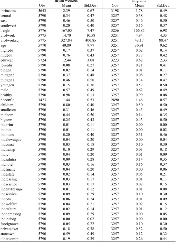
Table 1 lists the abbreviations and definition of all variables. Table 2 provides the descriptive statistics of the variables. The table illustrates the basic difference between an urban and a migrant worker. On average, urban workers received hourly wage RMB$10.91 with a age of 40.89 years old, 12.44 years of education, and 14.7 years of work experience; while migrants get hourly wage RMB$5.93 with 30.91 years of age, 9.62 years of education, and 4.94 years of work experience. Among them, 15% of urban workers with age below 30, while 57% of migrants aged below 30, and 31% of migrants workers work in manufacturing sector while only 20% of urban workers have job in manufacturing. Most of urban workers, 59%, employed in state-owned enterprises, while most of migrants, 52%, employed in private-owned
firms. In sum, the data show a general tendency that urban workers are (i) in average older than migrant workers, (ii) paid higher than migrant workers, (iii) better educated than migrants, (iv) more experienced than migrant workers, and (v) worked more in state-own enterprises than migrants who employed mostly in private enterprises.
[insert Tables 1-2 here]
IV. Estimation Results
Tables 3 and 4 respectively provide the results of Heckit test for both urban and migrant workers. Column (1) of the two tables is the base model, which regresses log hourly income on personal traits of employed agents. Column (2) to (5) of the two tables additionally adds the factor of geography, cohort, firm characteristics, and industry, separately to the base model. Column (6) jointly adds all the factors, geography, cohort, firm characteristics, and industry to the base model.
The six Heckit tests share the similar results. According to the first-stage selection results, an urban worker who are young or more self-confidence are more likely to be employed, while both variables are insignificant to determine the employment status of a migrant. This may be because migrants once decide to move they has a strong determination to work regardless of their age of confidence feeling. However, both urban agent and the migrant are male, have more education and better health condition tend to be employed. An urban agent who has the responsibility of child rearing is more likely to be employed. By contrast, a migrant rearing a child is less likely to find a job in a city because child rearing in city is more difficult and can be a burden for the migrant. As for geography and cohort, both are insignificant factors for determining employment status for the migrant; however, an urban in the east is more likely to find a job than in the central as eastern urban area provide better
labor conditions and job opportunities. Meanwhile, urban people of mid generation are more likely to be hired, while young generation of migrants exhibits advantage in finding a job in the city. Thus, the employment selection behavior for the urban and the migrant have some ways in common but also exist some discrepancies.
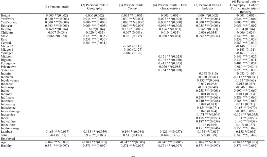
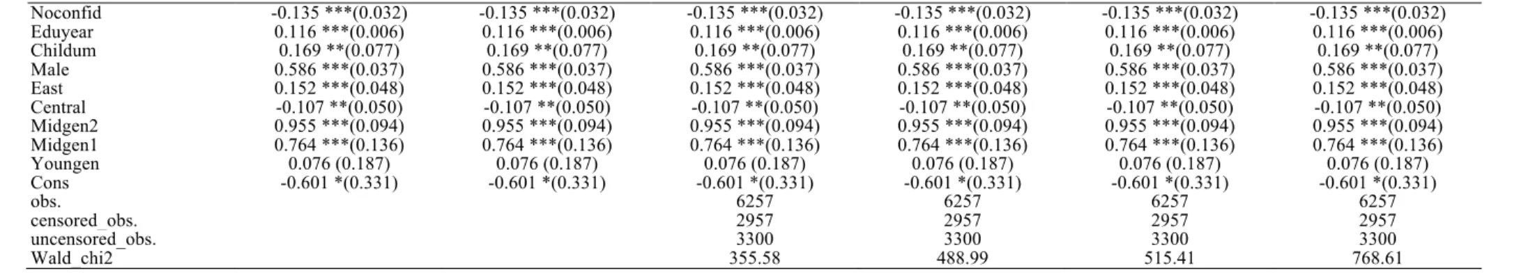
According to the second-stage results of income regression in Tables 3 and 4, sample correction terms derived from first stage are significant for wage determination of both urban and migrant workers, implying the necessity to correct for sample selection bias. The negative coefficient means that the observed wage tends to underestimate the real one. Both years of education and work experience are positive and strongly significant for both urban and migrant workers, but the returns to work experience of migrant workers are nearly twice the returns to work experience of urban workers implying that work experience is more important for those migrants who tend to be young, less educated and unskilled. Another reason is that the average years of work experience of the migrants is lower than that of urban workers. This result is thus consistent with law of diminishing returns. In fact, migrants in some occupation with the same years as that of urban workers, though paid lower than an urban worker, actually earns a higher rate of return to work experience. This support that the migrant relies more on skill accumulation through on-the-job training. It also implies that migrant workers’ human capital level in terms of work experience when compared to an urban worker is too low. In fact, the average work experience of the urban is about three times that of the migrants.
In contrast, the results show that urban workers have higher rate of returns to education than the migrants implying that urban workers enjoy more education resources than do migrant workers.7 After all, even if an urban worker has received
more years of education than a migrant worker, despite diminishing marginal returns, the rate of returns to his education level with better educational benefit and subsidy is still higher than that of a migrant worker without educational resources. The significant but negative estimates of squared value of work experience are consistent with nonlinear effect suggested by the literature.
Moreover, two other human capital variables, height and health condition, also show positive and significant effects on income level for both urban and migrant workers, and their effects are relatively stronger for the migrants than for the urban. This may have to do with the job characteristics that the migrants are engaged in work required more physical strength as in the manufacturing sector and at low operation level. All these results confirm that even in Chinese labor market human capital remains an important dimension for understanding the determination of labor income. Furthermore, except formal education which the urban has a great advantage over the migrants, other forms of human capital such as work experience and health condition the migrants have larger rates of return implying that improvement of human capital investment of the migrant can be an effective way to narrow the wage gap between urban and rural sectors.
As for geography, its coefficients are positive and significant; and, according to the magnitude, we find that for both urban and migrant workers their income level is higher in Eastern China and Central China than in Southwest China. This is consistent to our observation that job opportunity is better in these regions. In regard to the cohort effect, there is an evident difference between urban and migrant workers. For urban workers, there are no significant differences among cohorts, while for migrants, young workers tend to earn more and the highest income goes to the age group
between 30 and 45 years old. This implies that after controlling for personal traits, cohort does not influence urban agent’s income level but affect the migrant’s. We ascribe this phenomenon to relatively stable work environment in urban areas faced by urban workers with different cohorts. However, younger generation of migrants with more work experience tend to earn more implying either better job opportunities provided for them as the economy developed or better labor quality of new generation of migrants.
As for firm size, consistent with the literature, larger firms tend to pay higher wage. An urban worker receives a bigger wage premium in a medium-size company, while a migrant earns a highest wage premium from big company. This is because migrants usually work in big assembly factories as operation workers or laborers. For the type of firm ownership, both urban and migrant workers receive a highest wage premium from the foreign-owned company. However, in a private-owned company or a state-owned company only urban workers have a wage premium, while in a private-owned company where the migrant worker mostly worked it pays a negative wage premium, i.e., the migrant suffers a significant wage loss, implying that private firms are most likely to take the advantage of exploiting the migrant workers.
As for industry, urban workers tend to earn more in manufacturing; electric, water, and gas; information, computer, and software service; finance, real estate and leasing; scientific and technical service; education; health and social welfare; and domestic organization industries, while migrants earn more only in construction; information, computer, and software service; leasing; scientific and technical service; and education industries. The limited numbers of sectors that pay the migrants better wages implying that the migrants are likely segmented in the labor market.
[insert Tables 2-4 here]
Table 5 summarizes decomposition of income differentials. Tables 6 and 7 list unexplained and explained ratios. Group membership is not considered in Table 6 but is considered in Table 7.
Table 6 shows that our model specification in general explains up to 85-89%. When the urban is used as a reference group, the explained values of coefficient part are, in overall terms, larger than those of the case where the migrant is used as a reference group. Moreover, when geography, cohort, firm size, ownership and industry type are simultaneously added to the basic model, unexplained ratio can be reduced to 11% in the case where the urban is the reference group and to 15% in the case where the migrant is the reference group. The value of the unexplained ratio is close to that of Lee (2012) but smaller than that of Magnani and Zhu (2012).8
Columns (1) and (6) are the two baseline cases. Column (1) only considers personal traits, while column (6) considers personal traits, geography, cohort, firm characteristics and industry type simultaneously. According to column (1), we know that personal traits as a group of explanatory variables explain 76% of wage differential. The marginal effect of other variable groups, including geography, cohort, ownership and industry type added to the case of column (1), as column (6) shows, can only increase explained ratio by 13% in Panel I (making it increase from 76% in column (1) to 89% in column (6)) and by 14% in Panel II (making it increase from 71% in column (1) to 85% in column (6)). Therefore, personal traits are crucial to explaining the wage differential between urban and migrant workers.
8 Magnani and Zhu (2012) also point out that controlling for occupation and industry variables in
Among the other variable groups, the marginal contribution of cohort adding to personal traits has the greatest effect, since it increases explained ratios of column (1) by 9% in Panel I (improving it from 76% to 85%) and 11% in Panel II (improving it from 71% to 82%). By contrast, firm characteristics accounts for a least additional contribution, and geography and industry type share similar marginal effect.
Finally, let us look at the case where group membership is considered. As Table 7 shows, when group membership reflecting in the interception of regression models is considered as the unexplained part, the explained ratio will drop sharply from 70%-89% to 42%-60%. Meanwhile, we also find that cohort variable is least affected by the inclusion of group membership, since, when compared to the drop of geography, firm type and industry type, cohort solely added to column (1) brings about the smallest drop (from 85% in Panel I of Table 6 to 66% in Panel I of Table 7 and from 82% in Panel II of Table 6 to 60% in Panel II of Table 7). This implies that, when compared to other cases, the case considering cohort has a smaller effect of group members. Since group membership is a crucial component of unexplained ratio, we argue that the inclusion of cohort will increase explained ratio. By contrast, when geography, firm characteristics and industry type, are added to column (1) of Table 7, there shows no significant increase in explained ratio. This result implies that if discrimination towards migrants reflected in group membership, then the discrimination may largely be related to geography, firm ownership and industry type. These findings are consistent with that of Meng and Zhang (2001) and Appleton et al. (2004) who show significant labor market segregation and discrimination in occupation and industry to migrant workers in China.
By comparing the results from Table 6 and Table 7, we can conclude that including group membership will increase the unexplained part of wage differentials between the urban and migrant workers and it can be an approximation for total discrimination due to the Fukou system. However, the inclusion of industry type and firm characteristics variable in Table 6 reduces the unexplained part, which may underestimate the effect of discrimination as the migrants are restricted and segmented into certain occupation and industry sectors in the labor market.
V. Conclusion
Using Blinder-Oaxaca decomposition method, this study analyzes the influence of personal traits, geography, cohort, firm characteristics, and industry type on wage differential between urban and migrant workers. The results shows that, without considering unexplained part resulting from group membership, up to 85-89% of wage differentials in China’s labor market can be explained by personal traits, geography, cohort, firm characteristics, and industry type. And, if we solely look at the influence of personal traits on wage differential, we find that they explain 71-76% of the wage differential, which is consistent with the findings in Lee (2012). Among them, human capital variables are important factor determining one’s wage. On the other hand, if group membership is considered, the explained ratios drop prevalently in all the cases to 42-60%. However, among them, the case where cohort variable is added is least affected. This also suggest that the inclusion of firm characteristics and industry type variables without considering group membership is likely to underestimate the effect of discrimination as the migrants are subject to labor market discrimination and segregation by firms and industries. Likewise, the inclusion of
group membership can be a good approximation for estimation the total effect of discrimination in Chinese labor market.
In summery, our findings, on the one hand, imply that wage differential of China’s labor market is largely accounted for by the difference in human capital level, since personal traits such as education level, work experience, height, health condition are all crucial to determining wages. However, despite that migrants are subject to less educational resources and opportunity and hence receive less education and accumulate less work experience, they still have significant higher rates of return to health and work experience. Thus, policies towards the improvement in the human capital accumulation of the migrants can be an effective means to narrow the wage gap between rural and urban workers. On the other hand, we also find that the additional of cohort variable helps to increase explained ratio, whereas other factors such as geography, firm characteristics and industry type are more accountable for the discrimination towards migrants who are paid lower than the urban due to labor market segmentation. Thus model without considering group membership is likely to underestimate the effect of discrimination. The cohort effect may represent a better labor quality of new generations of migrants. However, the effect of group membership is likely the reflection of the current household registration (Fukou) system that not only discriminate the migrants in their identity and welfare benefits that the urban may acquire, but also on their children’s education opportunity and admission, which significantly impose an negative effect on the next generation of migrants. Thus, an institutional reform to abolish the Fukou system is perhaps the critical policy to close the income gap between rural and urban divide.
Table 1. Abbreviations and descriptions of variables
group of variable variable name explanation note Lhrincome log of hour wage
Employed being hired as a permanent worker, long term contract worker (one year and above) or a short term contract worker (less than one year)
personal traits Yrofwork years of work in present occupation Yrofworksq the square of years of work Eduyear years of education Age Years of age
Male gender dummy (male1 and female0)
Healthy dummy of good health (the value of dummy is 1 if the score of self-evaluation on health is between 1 and 3 otherwise its value is 0)
Noconfid dummy of “lacking self-confidence”
Childum dummy of children (1 if children number is greater than 0 and 0 otherwise)
geography Central dummy of central China southwest is the reference group East dummy of eastern China
Southwest dummy of southwestern China
cohort Oldgen dummy of old generation (aged above 60) oldgen is the reference group Midgen2 dummy of mid-generation (aged between 45 and 60)
Midgen1 dummy of mid-generation (aged between 30 and 45) Youngen dummy of young generation (aged below 30) firm characteristics Smallcom firm size dummy for small companies (with size
smaller than 50 persons) smallcom is the reference group Midcom firm size dummy for medium enterprises (with size
between 50 and 500 persons)
Bigcom firm size dummy for big company (with size no less than 500 persons)
Foreignown ownership dummy for “foreign-owned” Privateown ownership dummy for “private-owned” Stateown ownership dummy for “state-owned”
industry type Indprim industry dummy for “Agriculture, Forestry, Animal
husbandry, Fishery” indsalntra is the reference group Indmin industry dummy for “Mining”
Indmanu industry dummy for “Manufacturing”
Indelewatgas industry dummy for “Production and Supply of Electricity, Gas and Water”
Indconst industry dummy for “Construction Enterprise” Indtransp industry dummy for “Transport, Storage and Post
Industry”
Indict industry dummy for “Information Transmission, Computer Services and Software Industry” Indsalntra industry dummy for “Wholesale and Retail Trade” Indhotel industry dummy for “Hotel and Catering Services” Indfinanc industry dummy for “Financial Intermediation” Indestate industry dummy for “Real Estate Industry”
Indleasing industry dummy for “Leasing and Business Services” Indscience industry dummy for “Scientific Research, Technical
Service and Geologic Prospecting” Indenvtmange industry dummy for “Management of Water
Conservancy, Environment and Public Facilities” Indservice industry dummy for “Services to Households and
Other Services”
Indedu industry dummy for “Education”
Indwelfare industry dummy for “Health, Social Security and Social Welfare”
Indculture industry dummy for “Culture, Sport and Entertainment”
Inddomesorg industry dummy for “Public Management and Social Organization”
Table 2. Descriptive statistics
urban workers migrants
Obs Mean Std.Dev. Obs Mean Std.Dev. lhrincome 5643 2.39 0.67 3198 1.78 0.49 central 5790 0.34 0.47 3257 0.38 0.48 east 5790 0.46 0.50 3257 0.46 0.50 southwest 5790 0.20 0.40 3257 0.16 0.37 height 5776 167.05 7.47 3256 166.85 6.98 yrofwork 5775 14.70 10.58 3251 4.94 4.33 yrofworksq 5775 327.84 400.85 3251 43.17 88.47 age 5770 40.89 9.77 3251 30.91 9.62 highedu 5790 0.17 0.37 3257 0.02 0.14 midedu 5790 0.76 0.43 3257 0.77 0.42 eduyear 5724 12.44 3.08 3223 9.62 2.33 lowedu 5790 0.08 0.27 3257 0.21 0.41 oldgen 5790 0.02 0.14 3257 0.01 0.11 midgen2 5790 0.37 0.48 3257 0.08 0.27 midgen1 5790 0.46 0.50 3257 0.34 0.47 youngen 5790 0.15 0.36 3257 0.57 0.50 male 5790 0.57 0.49 3257 0.62 0.49 healthy 5790 0.98 0.13 3257 0.99 0.08 noconfid 3423 1.44 0.53 2890 1.46 0.57 childum 5790 0.80 0.40 3257 0.50 0.50 smallcom 5790 0.31 0.46 3257 0.43 0.49 midcom 5790 0.44 0.50 3257 0.14 0.35 bigcom 5790 0.25 0.43 3257 0.43 0.50 indprim 5790 0.01 0.11 3257 0.00 0.00 indmin 5790 0.01 0.11 3257 0.00 0.02 indmanu 5790 0.20 0.40 3257 0.31 0.46 indelewatgas 5790 0.04 0.20 3257 0.00 0.04 indconst 5790 0.03 0.18 3257 0.10 0.30 indtransp 5790 0.10 0.29 3257 0.03 0.18 indict 5790 0.04 0.20 3257 0.01 0.09 indsalntra 5790 0.09 0.28 3257 0.14 0.35 indhotel 5790 0.03 0.16 3257 0.16 0.37 indfinanc 5790 0.04 0.20 3257 0.00 0.06 indestate 5790 0.02 0.14 3257 0.05 0.21 indleasing 5790 0.03 0.17 3257 0.01 0.11 indscience 5790 0.03 0.17 3257 0.02 0.15 indenvtmange 5790 0.01 0.12 3257 0.01 0.08 indservice 5790 0.09 0.29 3257 0.10 0.30 indedu 5790 0.06 0.24 3257 0.01 0.09 indwelfare 5790 0.04 0.21 3257 0.02 0.15 indculture 5790 0.02 0.14 3257 0.01 0.12 inddomesorg 5790 0.09 0.29 3257 0.00 0.05 indintlorg 5790 0.00 0.02 3257 0.00 0.00 foreignown 5790 0.05 0.22 3257 0.10 0.30 privateown 5790 0.18 0.38 3257 0.52 0.50 stateown 5790 0.59 0.49 3257 0.12 0.32 othercomtp 5790 0.19 0.39 3257 0.26 0.44
Table 3. Income regression for urban workers
Dep var= lhrincome
(1) Personal traits (2) Personal traits + Geography (3) Personal traits + Cohort (4) Personal traits + Firm characteristics (5) Personal traits + Industry
(6) Personal traits + Geography + Cohort + Firm characteristics + Industry Height 0.005 **(0.002) 0.000 (0.002) 0.005 **(0.002) 0.003 (0.002) 0.004 *(0.002) -0.001 (0.002) Yrofwork 0.030 ***(0.004) 0.031 ***(0.004) 0.030 ***(0.004) 0.027 ***(0.004) 0.027 ***(0.004) 0.026 ***(0.004) Yrofworksq 0.000 ***(0.000) 0.000 ***(0.000) 0.000 ***(0.000) 0.000 ***(0.000) 0.000 ***(0.000) 0.000 ***(0.000) Eduyear 0.063 ***(0.005) 0.065 ***(0.005) 0.060 ***(0.006) 0.060 ***(0.005) 0.055 ***(0.005) 0.051 ***(0.007) Healthy 0.169 **(0.084) 0.162 *(0.084) 0.161 *(0.088) 0.186 **(0.083) 0.146 *(0.083) 0.134 (0.086) Childum -0.007 (0.034) -0.020 (0.033) 0.007 (0.041) 0.010 (0.033) 0.008 (0.034) -0.006 (0.039) Male 0.066 *(0.034) 0.123 ***(0.035) 0.061 (0.039) 0.080 **(0.034) 0.092 ***(0.034) 0.140 ***(0.040) East 0.251 ***(0.030) 0.238 ***(0.029) Central 0.284 ***(0.031) 0.283 ***(0.030) Midgen2 -0.146 (0.115) -0.146 (0.118) Midgen1 -0.100 (0.127) -0.143 (0.131) Youngen -0.089 (0.126) -0.163 (0.129) Midcom 0.151 ***(0.025) 0.143 ***(0.025) Bigcom 0.102 ***(0.030) 0.133 ***(0.031) Foreignown 0.411 ***(0.055) 0.401 ***(0.054) Privateown 0.076 **(0.035) 0.080 **(0.034) Stateown 0.164 ***(0.028) 0.127 ***(0.028) Indmin -0.098 (0.110) -0.083 (0.107) Indmanu -0.060 (0.041) -0.112 ***(0.041) Indelewatgas 0.135 **(0.064) 0.113 *(0.063) Indconst 0.037 (0.068) 0.018 (0.067) Indtransp -0.003 (0.048) -0.046 (0.048) Indict 0.258 ***(0.061) 0.197 ***(0.060) Indhotel 0.001 (0.075) 0.013 (0.073) Indfinanc 0.298 ***(0.061) 0.289 ***(0.060) Indestate 0.240 ***(0.086) 0.285 ***(0.083) Indleasing 0.094 (0.073) 0.111 (0.071) Indscience 0.154 **(0.071) 0.163 **(0.070) Indenvtmange 0.046 (0.094) -0.009 (0.092) Indservice -0.171 ***(0.046) -0.121 ***(0.045) Indedu 0.155 ***(0.053) 0.131 **(0.053) Indwelfare 0.187 ***(0.059) 0.145 **(0.059) Indculture 0.116 (0.079) 0.109 (0.077) Inddomesorg 0.151 ***(0.046) 0.155 ***(0.048) Lambda -0.165 ***(0.057) -0.153 ***(0.059) -0.194 **(0.084) -0.125 **(0.057) -0.134 **(0.057) -0.158 *(0.092) cons 0.444 (0.385) 0.939 **(0.383) 0.611 (0.452) 0.464 (0.379) 0.592 (0.379) 1.343 ***(0.449) Employed Age -0.047 ***(0.005) -0.047 ***(0.005) -0.047 ***(0.005) -0.047 ***(0.005) -0.047 ***(0.005) -0.047 ***(0.005) Healthy 0.571 ***(0.097) 0.571 ***(0.097) 0.571 ***(0.097) 0.571 ***(0.097) 0.571 ***(0.097) 0.571 ***(0.097)
Noconfid -0.135 ***(0.032) -0.135 ***(0.032) -0.135 ***(0.032) -0.135 ***(0.032) -0.135 ***(0.032) -0.135 ***(0.032) Eduyear 0.116 ***(0.006) 0.116 ***(0.006) 0.116 ***(0.006) 0.116 ***(0.006) 0.116 ***(0.006) 0.116 ***(0.006) Childum 0.169 **(0.077) 0.169 **(0.077) 0.169 **(0.077) 0.169 **(0.077) 0.169 **(0.077) 0.169 **(0.077) Male 0.586 ***(0.037) 0.586 ***(0.037) 0.586 ***(0.037) 0.586 ***(0.037) 0.586 ***(0.037) 0.586 ***(0.037) East 0.152 ***(0.048) 0.152 ***(0.048) 0.152 ***(0.048) 0.152 ***(0.048) 0.152 ***(0.048) 0.152 ***(0.048) Central -0.107 **(0.050) -0.107 **(0.050) -0.107 **(0.050) -0.107 **(0.050) -0.107 **(0.050) -0.107 **(0.050) Midgen2 0.955 ***(0.094) 0.955 ***(0.094) 0.955 ***(0.094) 0.955 ***(0.094) 0.955 ***(0.094) 0.955 ***(0.094) Midgen1 0.764 ***(0.136) 0.764 ***(0.136) 0.764 ***(0.136) 0.764 ***(0.136) 0.764 ***(0.136) 0.764 ***(0.136) Youngen 0.076 (0.187) 0.076 (0.187) 0.076 (0.187) 0.076 (0.187) 0.076 (0.187) 0.076 (0.187) Cons -0.601 *(0.331) -0.601 *(0.331) -0.601 *(0.331) -0.601 *(0.331) -0.601 *(0.331) -0.601 *(0.331) obs. 6257 6257 6257 6257 censored_obs. 2957 2957 2957 2957 uncensored_obs. 3300 3300 3300 3300 Wald_chi2 355.58 488.99 515.41 768.61
Note: Significance level: 1%=***, 5%=** and 10%=*. For abbreviations, see Table 3.
Table 4. Income regression for migrant workers
Dep var= lhrincome
(1) Personal traits (2) Personal traits + Geography (3) Personal traits + Cohort (4) Personal traits + Firm characteristics (5) Personal traits + Industry geography + cohort + firm (6) on personal traits + characteristics + industry Height 0.010 ***(0.002) 0.006 ***(0.002) 0.010 ***(0.002) 0.009 ***(0.002) 0.010 ***(0.002) 0.006 ***(0.002) Yrofwork 0.058 ***(0.005) 0.051 ***(0.005) 0.053 ***(0.005) 0.051 ***(0.005) 0.055 ***(0.005) 0.042 ***(0.005) Yrofworksq -0.002 ***(0.000) -0.002 ***(0.000) -0.002 ***(0.000) -0.002 ***(0.000) -0.002 ***(0.000) -0.001 ***(0.000) Eduyear 0.055 ***(0.004) 0.058 ***(0.003) 0.055 ***(0.004) 0.051 ***(0.004) 0.053 ***(0.004) 0.053 ***(0.003) Healthy 0.191 *(0.101) 0.185 *(0.097) 0.208 **(0.101) 0.186 *(0.098) 0.154 (0.099) 0.163 *(0.094) Childum 0.003 (0.018) 0.020 (0.018) -0.055 **(0.025) -0.001 (0.018) -0.009 (0.018) -0.015 (0.023) Male 0.004 (0.026) 0.055 **(0.025) -0.114 ***(0.037) 0.018 (0.025) -0.024 (0.026) -0.049 (0.032) East 0.361 ***(0.023) 0.312 ***(0.026) Central 0.261 ***(0.024) 0.190 ***(0.026) Midgen2 0.448 ***(0.112) 0.388 ***(0.098) Midgen1 0.697 ***(0.121) 0.619 ***(0.106) Youngen 0.459 ***(0.111) 0.464 ***(0.096) Midcom 0.005 (0.025) -0.015 (0.024) Bigcom 0.116 ***(0.018) 0.077 ***(0.019) Foreignown 0.160 ***(0.031) 0.116 ***(0.031) Privateown -0.052 ***(0.019) -0.026 (0.018) Stateown 0.008 (0.028) 0.012 (0.027) Indmin 0.357 (0.442) 0.350 (0.427) Indmanu 0.144 ***(0.025) 0.040 (0.026) Indelewatgas 0.223 (0.219) 0.090 (0.209) Indconst 0.144 ***(0.034) 0.103 ***(0.033) Indtransp 0.060 (0.048) 0.009 (0.046)
Indict 0.185 **(0.090) 0.156 *(0.086) Indhotel -0.118 ***(0.028) -0.102 ***(0.027) Indfinanc 0.089 (0.123) 0.127 (0.118) Indestate 0.029 (0.041) 0.046 (0.040) Indleasing 0.245 ***(0.072) 0.232 ***(0.069) Indscience 0.139 **(0.055) 0.104 **(0.052) Indenvtmange -0.025 (0.103) -0.045 (0.099) Indservice -0.025 (0.032) -0.054 *(0.031) Indedu 0.115 (0.090) 0.111 (0.086) Indwelfare -0.090 (0.057) -0.129 **(0.054) Indculture 0.087 (0.068) 0.095 (0.064) Inddomesorg -0.264 *(0.147) -0.355 **(0.140) Lambda 0.009 (0.069) 0.120 *(0.067) -0.755 ***(0.146) 0.075 (0.068) 0.049 (0.068) -0.411 ***(0.132) Cons -0.779 ***(0.292) -0.518 *(0.283) -0.482 (0.324) -0.725 **(0.286) -0.840 ***(0.286) -0.376 (0.298) Employed Age -0.004 (0.005) -0.004 (0.005) -0.004 (0.005) -0.004 (0.005) -0.004 (0.005) -0.004 (0.005) Healthy 0.622 ***(0.162) 0.622 ***(0.162) 0.622 ***(0.162) 0.622 ***(0.162) 0.622 ***(0.162) 0.622 ***(0.162) Noconfid 0.008 (0.029) 0.008 (0.029) 0.008 (0.029) 0.008 (0.029) 0.008 (0.029) 0.008 (0.029) Eduyear 0.100 ***(0.008) 0.100 ***(0.008) 0.100 ***(0.008) 0.100 ***(0.008) 0.100 ***(0.008) 0.100 ***(0.008) Childum -0.295 ***(0.053) -0.295 ***(0.053) -0.295 ***(0.053) -0.295 ***(0.053) -0.295 ***(0.053) -0.295 ***(0.053) Male 0.214 ***(0.029) 0.214 ***(0.029) 0.214 ***(0.029) 0.214 ***(0.029) 0.214 ***(0.029) 0.214 ***(0.029) East 0.022 (0.041) 0.022 (0.041) 0.022 (0.041) 0.022 (0.041) 0.022 (0.041) 0.022 (0.041) Central 0.023 (0.042) 0.023 (0.042) 0.023 (0.042) 0.023 (0.042) 0.023 (0.042) 0.023 (0.042) Midgen2 -0.226 (0.188) -0.226 (0.188) -0.226 (0.188) -0.226 (0.188) -0.226 (0.188) -0.226 (0.188) Midgen1 -0.196 (0.211) -0.196 (0.211) -0.196 (0.211) -0.196 (0.211) -0.196 (0.211) -0.196 (0.211) Youngen 0.628 ***(0.048) 0.628 ***(0.048) 0.628 ***(0.048) 0.628 ***(0.048) 0.628 ***(0.048) 0.628 ***(0.048) Cons -1.565 ***(0.089) -1.565 ***(0.089) -1.565 ***(0.089) -1.565 ***(0.089) -1.565 ***(0.089) -1.565 ***(0.089) obs. 8325 8325 8325 8325 8325 8325 censored_obs. 5169 5169 5169 5169 5169 5169 uncensored_obs. 3156 3156 3156 3156 3156 3156 Wald_chi2 532.09 811.37 558.54 703.93 735.06 1055.64
Table 5. Summary of income differential decomposition
(1)
personal traits (1)+geography (2)
(3) (1)+cohort (4) (1)+ firm type (size and ownership) (5) (1)+ industry type (6) all included urban as reference A: coefficient; explained. 0.33 0.32 0.31 0.36 0.35 0.34 B: coefficient; unexplained -0.84 -0.97 -1.42 -0.79 -1.04 -1.76 C: constant; unexplained 1.22 1.46 1.09 1.19 1.43 1.72 migrant as reference A: coefficient; explained. 0.19 0.19 0.20 0.20 0.17 0.16 B: coefficient; unexplained -0.71 -0.84 -1.32 -0.64 -0.87 -1.58 C: constant; unexplained 1.22 1.46 1.09 1.19 1.43 1.72
Table 6. Unexplained and explained ratios (without group membership)
(1)
personal traits (1)+geography (2) (1)+cohort (3)
(4) (1)+ firm type (size and ownership) (5) (1)+ industry type (6) all included Panel I. urban as reference
exp(A)/(exp(A)+exp(B)) 76% 78% 85% 76% 80% 89%
exp(B)/(exp(A)+exp(B)) 24% 22% 15% 24% 20% 11%
Panel II. migrant as reference
exp(A)/(exp(A)+exp(B)) 71% 74% 82% 70% 74% 85%
exp(B)/(exp(A)+exp(B)) 29% 26% 18% 30% 26% 15%
Table 7. Unexplained and explained ratios (with group membership)
(1) personal traits (2) (1)+geography (3) (1)+cohort (4) (1)+ firm type (size and ownership) (5) (1)+ industry type (6) all included Panel I. urban as ref
exp(A)/(exp(A)+exp(B+C)) 49% 46% 66% 49% 49% 60% exp(B+C)/(exp(A)+exp(B+C)) 51% 54% 34% 51% 51% 40% Panel II. migrant as reference
exp(A)/(exp(A)+exp(B+C)) 42% 40% 60% 41% 40% 51% exp(B+C)/(exp(A)+exp(B+C)) 58% 60% 40% 59% 60% 49%
References
Allen, S. G. (1991) “Technology and the Wage Structure,” Mimeo. North Carolina State University.
Altonji, J.G. and Blank R. (1999) “Race and Gender in the Labor Market,” In Ashenfelter, O. and Card, D. (Eds.), Handbook of Labor Economics, Vol. 3C, Elsevier Science B.V., pp. 3143-3259.
Appleton, S., Knight J., Song L., and Xi Q. (2004) “Contrasting Paradigms: Segmentation and Competitiveness in the Formation of the Chinese Labor Market,” Journal of Chinese Economic and Business Studies, 2 (3), pp.185–205 Beaudry, P. and Green, D. (2005) “Changes in U.S. Wages, 1976-2000: Ongoing
Skill Bias or Major Technological Change?” Journal of Labor Economics, 23, 3, pp. 609-48.
Blinder, A.S. (1973) “Wage Discrimination: Reduced Form and Structural Estimates,”
Journal of Human Resources, 8, pp. 436-454.
Bound, J., and Johnson, G. (1992) “Changes in the Structure of Wages during the 1980s: An Evaluation of Alternative Explanations,” American Economic Review, LXXXII, pp. 371-92.
Forbes, K. (2001) “Skill Classification Does Matter: Estimating the Relationship between Trade Flows and Wage Inequality,” Journal of International Trade &
Economic Development, 10 (2), pp. 175-209.
Heckman, J. (1979):“Sample Selection Bias as a Specification Error,” Econometrica, 47(1): pp. 153-61.
Heckman, J. (1998) “Detecting Discrimination,” Journal of Economic Perspectives, 12(2), pp. 101-116.
Jones, F. L., and Kelley, J. (1984) “Decomposing Differences between Groups. A Cautionary Note on Measuring Discrimination,” Sociological Methods and
Research, 12, pp. 323-343.
Krueger, A. (1993) “How Computers Changed the Wage Structure: Evidence from Microdata, 1984-1989,” Quarterly Journal of Economics, 108, 1, pp. 33-60. Lee, L. (2012) “Decomposing Wage Differentials between Migrant Workers and
Urban Workers in Urban China's Labor Markets,” China Economic Review, 23(2), pp. 461-470.
Liu, P.W., Meng, X., and Zhang J. (2000) “Sectoral Gender Wage Differentials and Discrimination in the Transitional Chinese Economy,” Journal of Population
Economics, 13(2), pp. 331-352.
Magnani, E. and Zhu, R. (2012) “Gender Wage Differentials among Rural–urban Migrants in China,” Regional Science and Urban Economics, 42 (5), pp. 779-793.
Meng, X. (2012) ”Labor Market Outcomes and Reforms in China,” Journal of
Economic Perspectives, 26(4), pp. 75-101
Meng, X. and Zhang, J. (2001) “The Two-Tier Labor Market in Urban China: Occupational Segregation and Wage Differentials between Urban Residents and Rural Migrants in Shanghai,” Journal of Comparative Economics, 29(3), pp. 485-504.
Mincer, J. (1991) “Human Capital, Technology, and the Wage Structure: What Do Time Series Show?” NBER Working Paper No. 3581.
Oaxaca, R. (1973) “Male-female Differentials in Urban Labor Markets,” International
Economic Review, 14. pp. 693-709.
Wage Differentials,” Journal of Econometrics, Vol. 61, pp. 5-21.
Park, Albert (2007) “Rural-Urban Inequality,” in S. Yusuf and T. Saich (eds), China in China Urbanizes: Consequences, Strategies, and Policies, Washington, D.C.: the World Bank.
Rozelle, S., Dong, X.-Y., Zhang, L., and Mason, A. (2002) “Gender Wage Gaps in Post-Reform rural China,” Pacific Economic Review, 7(1), pp157-179.
Appendix Proof of equation (3)
Consider the case where migrant is used as a reference group, wage differential can be expressed as
INC!− INC!
= (e!!′!!− e!!′!!)
= e!!′!!(e(!!′!!!!!′!!)!(!!′!!!!!′!!)− 1)
= INC!(e(!!′!!!!!′!!)!(!!′!!!!!′!!)− 1), which can be alternatively expressed as
(INC!− INC!)/INC!= e!!′(!!!!!)e(!!′!!!′)!!− 1.
This equation describes wage differential between urban and migrant workers as a deviation from the average wage level of migrant workers, INC!. We treat X!′− X!′ , β!− β! and (X!′β!− X!′β!) + (X!′β!− X!′β!) as three sources of the deviation so we decompose the deviation as three parts influenced by the three factors. We give each part an equal weight so e!!′(!!!!!)e(!!′!!!′)!! can be
expressed as a summand of
(i) e!!′(!!!!!)e(!!′!!!′)!! where X
!′ = X!′ , β! ≠ β! and (X!′β!− X!′β!) + (X!′β!− X!′β!) ≠ 0,
(ii) e!!′(!!!!!)e(!!′!!!′)!! where X!′ ≠ X!′ , β! = β! and (X!′β!− X!′β!) +
(X!′β!− X!′β!) ≠ 0, and
(iii) e!!′(!!!!!)e(!!′!!!′)!! where X!′ ≠ X!′ , β! ≠ β! and (X!′β!− X!′β!) +
(X!′β!− X!′β!) = 0.
Thus, (INC!− INC!)/INC! = [e!!′(!!!!!)e !!′!!!′ !!|
!!′ !!!′+ e!!′(!!!!!)e(!!′!!!′)!!| !!!!! + e !!′(!!!!!)e(!!′!!!′)!!| !!′ (!!!!!)!!(!!′!!!′)!!)]/ 3 − 1 ∝ e!!′(!!!!!)+ e(!!′!!!′)!!.
科技部補助專題研究計畫項下出席國際學術會議心得報告
日期:2015 6 月 7 日
一、
加會議經過
This 1st Annual International Conference on Social Sciences held in the historical and economically thriving city also the end of ancient Silk Road, Istanbul, Turkey. This conference was organized by Yuldiz Technical University found in 1911 and one of the leading university with a history over one hundred years old in Turkey. This conference aims to bring together researchers, scientists, scholars and students to exchange and share their experiences, new ideas, and research results about economics (economic theory, economic analysis, macroeconomics and money, microeconomics, economic psychology, econometrics, international economics, public finance, economic growth and development, social economics), business and administrative studies (management, marketing, finance and accounting, international business, supply chain and logistics management) within the global and interdisciplinary scope, and discuss the practical challenges encountered and the solutions proposed. This three-day conference was well organized by the host university with many sessions across different areas of economic studies. In addition to the ordinary sessions, the
計畫編號 MOST 103-2410-H-004 -015 - 計畫名稱 中國農民工遷移、就業選擇與區隔及與城市勞工薪資差異之研究 出國人員姓 名 莊奕琦 服務機構及職稱 政治大學經濟學系 教授 會議時間 104 5月21日至104 5月23日 會議地點 Istanbul, Turkey 會議名稱 (中文) 第1屆社會科學國際年會
(英文) 1st Annual International Conference on Social Sciences
(AICSS)
發表 文題
目 (中文) 決定中國農民工與城市居民薪資的差異原因探討
(英文) Behind the Invisible Wall: What Determines Wage Differentials between Urban and Migrant Workers in China
Professor Erdener Kaynak, School of Business Administration at the Pennsylvania State University shed important light on the recent development of the trend of globalization and regional development and its implications for the 21st century. His predictions are as fellows. Changing technologies and rapid innovations will prevail. Technological connectivity is transforming the way people live and interact. The unprecedented aging of population across the developed world will call for new level of efficiency and creativity from the public sector. The collapse of central planned economies in Eastern/central Europe has created a paradigm shift in global development, business, and investment. Europe as single market and South-East Asia is a growth market as an economic force to reckon with. This keynote speech gave us the comprehensive view on the future global trends and world development and its effects on regionalism. Except NAFTA, Europe and Asia are going to be two important regions for the growth of world economy. His predictions in some parts are consistent with my observations, however, he did not make a prediction on the rise of China and the recent initiative of “One Belt, One Road” development strategy through traditional land and maritime silk roads by Chairman Xi of PRC, which I believe will generate profound effect on Asia and Europe in long-term perspective. In order to enhance the relationship among all participants, this conference offered a Gala Dinner in a resort restaurant located in the traditional historical place, Cemile Sultan Korusu. People are able to relax, discuss, and share research results with each other before and during the dinner. Each of the three plenary sessions was designed and conducted in small size so that it enables participants to have closer discussion and focus on the presented papers. Overall, although this is a first year annual conference but I think it is a very well-organized and successful international conference and participants can have more time to share views on their opinions.
二、與會心得
Being a Taiwan scholar, I found this multidisciplinary international conference a wonderful opportunity for me to attend, to interchange, and to share the academic ideas, the expertise, and experience with distinguished scholars from different disciplines and countries. I presented a paper on “Behind the Invisible Wall: What Determines Wage Differentials between Urban and Migrant Workers in China” at the session of Labor Issues. My paper intends to identify the sources of the wage differentials between migrant workers and urban workers in China. Using a wider scope of city data from a 2008 survey of Rural-Urban Migration in China, our work employs a comprehensive aspect of explanatory variables to empirically estimate wage determination and decomposes the wage differentials between urban and migrant workers in the Chinese labor market. We find that personal traits, geography, cohort, firm characteristics, and industry type