Game Theory at Grace Baptist Church 貳

Game Theory at Grace Baptist Church

Spring 2006

Professor Hsueh-I Lu （呂學一）

National Taiwan University

重要的規定（將會每週提醒）

重要的規定（將會每週提醒）



除了白開水之外，禁止在教室內飲食，

違者立刻喪失旁聽與修課的資格。



注意路上的安全，過馬路時不要趕時間

，我們上課不會點名，所以遲到，缺席

都沒有關係，就是千萬不要「用生命趕

路」。



盡可能將腳踏車停在校園內然後走過來

，以免造成懷恩堂周遭環境的紊亂。

Outline

Outline



Strategic games



Nash equilibrium



Strictly competitive games



Bayesian games



上官與左左木兩位同學涉嫌於期末考聯

手舞弊，遭隔離偵訊

_…

An example

An example

上招

上不招

左招

各記大過一次

左小過、上退學

左不招 上小過、左退學

都沒事

Strategic games

Strategic games



Also known as

– Matrix games

– Games in normal form

Choices

Choices



In a strategic game,

– (1) each player chooses her plan of action

once and for all, and

– (2) all players make their choices

simultaneously.



An equivalent implementation for (2):

– When each player makes her choices, she is

not aware of other players’ choices.

Players

Players

上招

上不招

左招

各記大過一次

左小過、上退學

左不招 上小過、左退學

都沒事

F

There are always a ¯nite number n ¸ 2 of players in

a game.

F

_{Let N = f 1;2;:::;ng denote the set of players. For}

example, thefollowing is a 2-player game. Sometime,

we call them the

row player

and the

column player

.

Actions

Actions

上招

上不招

左招

各記大過一次

左小過、上退學

左不招 上小過、左退學

都沒事

F

Each player may have an arbitrary number of actions. A

game is

¯nite

if the number of actions for each player is

¯nite.

F

_{Let A = A}

₁

£ A

₂

£ ¢¢¢£ A

_n

denote the set possible actions.

F

For example, in the following game, each player has two

actions. We have jA

₁

_{j = jA}

₂

_{j = 2 and thus jAj = 2¢2 = 4.}

Consequences

Consequences

上招

上不招

左招

各記大過一次

各記小過一次

左不招

各記小過一次

都沒事

F

Let C consist of all possible consequences of

the game.

F

Each action is associated with a consequence.

F

For example, thefollowing gamehas only three

possible consequences.

Preference on consequences

Preference on consequences

上招

上不招

左招

c

₁

: 各記大過一次

c

₂

: 各記小過一

次

左不招

c

₂

: 各記小過一

次

c

₃

: 都沒事

F

The preference of each player on C is a total order.

F

For two consequences c and d in C, let c %

_i

d signify

that the i-th player does not prefer d to c.

F

For example c

₃

%

_i

c

₂

%

_i

c

₁

_{holds for i = 1;2 in the}

following game.

Preference on actions

Preference on actions

上 Confess

上 Deny

左

Confess

c

1

: 各記大過一次

c

2

: 各記小過一

_次

左 Deny

c

₂

: 各記小過一

次

c

₃

: 都沒事

F

The preference of each player on A is a total order.

F

For two actions a and bin A, let a %

_i

bsignify c(a) %

_i

c(b), where c(a) and c(b) are the consequences of a

and b, respectively.

F

For example, (Deny;Deny) %

₁

(Confess;Deny) %

₁

(Confess;Confess).

Utility (or payoff)

Utility (or payoff)

F

Usually, the preference relation is represented by a

utility (or payo®) function.

上招

上不招

左招

各記大過一次

左小過、上退學

左不招 上小過、左退學

都沒事

上招

上不招

左招

(-5,-5)

(-2,-10)

左不招

(-10,-2)

(0,0)

F

(0;0) %

₁

(¡ 2;¡ 10) %

₁

(¡ 5;¡ 5) %

₁

(¡ 10;¡ 2).

F

(0;0) %

₂

(¡ 10;¡ 2) %

₂

(¡ 5;¡ 5) %

₂

(¡ 2;¡ 10).

Some classic games

Some classic games

Confess or Deny

Confess or Deny

上招

上不招

左招

(-5,-5)

(-2,-10)

左不招

(-10,-2)

(0,0)

Prisoner’s Dilemma

Prisoner’s Dilemma

上招

上不招

左招

(-5,-5)

(

2

,-10)

左不招

(-10,

2

)

(0,0)

Brokeback or Crash

Brokeback or Crash

Brokeback

Mountain

Crash

Brokeback

Mountain

2,1

0,0

Crash

0,0

1,2

Its classic

name: “battle

of sexes”.

Hawk-Dove

Hawk-Dove

Dove

Hawk

Dove

3,3

1,4

Matching pennies

Matching pennies

Front Back

Front

1,-1

-1,1

Back

-1,1

1,-1

Chemistry

Nash equilibrium

Nash equilibrium

Also known as saddle point,

steady state, and local optimum.

Origin

Origin



The concept of the Nash equilibrium

was originated by Nash in his

dissertation, Non-cooperative games

(1950).



Nash showed that the various

solutions for games that had been

Roughly speaking

Roughly speaking



An action of a game is a Nash equilibrium

if each player has no incentive to change

her action under the assumption that all

the other players do not change their

Formally,

Formally,

An action a

¤

_{= (a}

¤

1

;a

¤

2

;:::;a

¤

n

) is a

Nash equilibrium

of the game if

a

¤

_%

i

(a

¤

₁

;a

¤

₂

;:::;a

¤

_{i ¡ 1}

;

a

i

;a

¤

_{i +1}

;:::;a

¤

_n

)

holds for each i 2 N and each action a

_i

2 A

_i

.

上招

上不招

左招

(-5,-5)

(-2,-10)

左不招

Prisoner’s Dilemma

Prisoner’s Dilemma

上招

上不招

左招

(-5,-5)

(

2

,-10)

左不招

(-10,

2

)

(0,0)

Brokeback or Crash

Brokeback or Crash

Brokeback

Mountain

Crash

Brokeback

Mountain

2,1

0,0

Crash

0,0

1,2

Hawk-Dove

Hawk-Dove

Dove

Hawk

Dove

3,3

1,4

Front Back

Front

1,-1

-1,1

Back

-1,1

1,-1

Matching pennies

Matching pennies

Chemistry

An infinite game

An infinite game



A first-price auction

畢卡索的油畫

畢卡索的油畫

《拿煙斗的男孩

《

拿煙斗的男孩

》

_》

(Garcon al la Pipe)

_{(Garcon al la Pipe)}

，以

，以

1

₁

億

_億

416

416

萬美元的天價售出，一舉刷新繪畫作品拍賣的世界記錄，成為

萬美元的天價售出，一舉刷新繪畫作品拍賣的世界記錄，成為

目前世界上最昂貴的畫。

Settings

Settings

F

Let v

_i

be thevaluation of thepainting for thei-th player such that

v

₁

> v

₂

> ¢¢¢> v

n

> 0:

T he set of actions for each player is [0;1 ). T herefore, it is an

in¯nite game.

F

Suppose that b

_i

is the bid of the i-th player. If

b

_i

_{= max}

1· j · n

b

j

and b

_j

< b

_i

holds for each j < i, then the payo®for the i-th player

is v

_i

¡ b

_i

. Otherwise, the payo®for the i-th player is 0.

Question

Question

What are the Nash equilibria of the

game?

Nash equilibria

Nash equilibria

The Nash equilibria consist of the actions b such that

F

C1: v

₂

· b

₁

· v

₁

;

F

C2: b

_j

· b

₁

holds for all j > 1; and

F

C3: there is an index j > 1 with b

_j

_{= b}

₁

.

We show that Conditions C1, C2, and C3 together imply that b

is a Nash equilibrium

F

By C2, player 1 always wins. Therefore, the payo®is

(v

₁

¡ b

₁

;0;0;:::;0):

F

Player 1 does not want to change her bid. Why?

If player k wins the bid

If player k wins the bid

The Nash equilibria consist of the actions b such that

F

C1: v

₂

· b

₁

· v

₁

;

F

C2: b

_j

· b

₁

holds for all j > 1; and

F

C3: there is an index j > 1 with b

_j

_{= b}

₁

.

The payo®of player k with a bid ^

b

_k

> b

₁

is

Nash equilibria

Nash equilibria

T he Nash equilibria consist of the actions b such that

F

C1: v

₂

· b

₁

· v

₁

;

F

C2: b

_j

· b

₁

holds for all j > 1; and

F

C3: there is an index j > 1 with b

_j

_{= b}

₁

.

T he direction that

b is a Nash equilibrium implies Conditions C1, C2, and C3

is left as an exercise.

Comments

Comments



The aforementioned game for first-price

auction describes the situation that all

players know the valuations of all players.



If some valuations are unknown to some

players, the first-price auction should be

modeled as a Bayesian game, to be

Second-price auction

Second-price auction



A second-price auction is also

known as Vickery auction, named

after William Vickery, who received

the Nobel prize in 1996.

– Vickery is recognized as the founder of

auction theory.

– Vickery is the first one discovered that

bidding the valuation is a dominant

Dominant strategy

Dominant strategy

上招

上不招

左招

(-5,-5)

(2,-10)

左不招

(-10,2)

(0,0)

The column player’s

dominant strategy

The row player’s

dominant strategy

The game

The game

F

Let v

_i

be the valuation for the i-th player such that

v

₁

> v

₂

> ¢¢¢> v

n

> 0:

T he set of actions for each player is [0; 1 ). So, it is an in¯nite

game.

F

Suppose that, for each j with 1 · j · n, b

_j

is the bid of the j -th

player. If i is the index such that (1) b

_i

_{= max}

_{1· j · n}

b

_j

, and (2)

b

_j

< b

_i

holds for each j with 1 · j < i, then the payo®for the i-th

player is

v

_i

¡

max

1· j · n;j 6

=i

b

j

:

Vickery’s Finding

Vickery’s Finding

Letting b

_i

_{= v}

_i

is a

(weakly) dominant strategy

for each player i.

That is, the payo®of the i-th player for the bid b with b

_i

_{= v}

_i

is

no worse than the payo®of the i-th player for any bid ^

bsuch that

^

_b

_j

_{= b}

_j

_{holds for each j 6}

_{= i.}

(Why?)

An observation: If b

_i

_{= v}

_i

, then the i-th player has non-negative

payo®in the second-price auction.

Case analysis – (1)

Case analysis – (1)

Case 1: max

_{j 6}

_=i

b

_j

¸ v

_i

.

F

If the i-th player loses the painting with ^

b, the

payo®of ^

b is zero, no better than that of b.

F

If thei-th player wins thepainting with ^

b, then

^

_b

_i

_{> v}

_i

_{. The second price is at least v}

_i

_.

There-fore, the payo®of ^

b for the i-th player is at

most zero.

Case analysis – (2)

Case analysis – (2)

Case 2: max

_{j 6}

_=i

b

_j

< v

_i

.

With b, the i-th player wins the painting and pays

the price max

_{j 6}

_=i

b

_j

.

F

If the i-th player loses the painting with ^

b, the

payo®of ^

b is zero, no better than that of b.

F

If thei-th player wins thepainting with ^

b, then

the i-th player still pays the price max

_{j 6}

_=i

b

_j

.

Her payo®does not change.

Comments (again)

Comments (again)



The aforementioned game for

second-price auction describes the situation that

all players know the valuations of all

players.



If some valuations are unknown to some

players, the second-price auction should

be modeled as a Bayesian game, to be

discussed later.

Strictly competitive games

Strictly competitive games

Definition

Definition

A two-player game is

strictly competitive

if

a %

₁

b if and only if b%

₂

a

Questions

Questions

Let u be the payo®(i.e., utility) function of a two-player

strictly competitive game. The de¯nition says that

u

₁

(a) ¸ u

₁

(b) if and only if u

₂

(b) ¸ u

₂

(a)

holds for any two actions a and b of the game.

Do the following conditions hold as well?

F

u

₁

_{(a) = u}

₁

(b) if and only if u

₂

_{(a) = u}

₂

(b)?

A popular name

A popular name

Definition

Definition

Let u be the payo®(i.e., utility) function of a two-player game. The

game is

zero-sum

if

u

₁

(a) + u

₂

_{(a) = 0}

holds for any action a 2 A of the game.

Question

Question

Are two definitions the same?

Otherwise, why a strictly competitive game

is known as a zero-sum game?

How they relate?

How they relate?

Any two-player strictly competitive game admits a

payo®function u to represent its preference relation

such that u

₁

(a) +u

₂

_{(a) = 0 holds for any action a of}

the game.

Focus on zero-sum games

Focus on zero-sum games



The rest of the discussion for strictly

competitive games focuses on zero-sum

games.



It suffices to specify the payoff of one

player (e.g., the row player) in a zero-sum

game.

– The row player is the maximizer.

Maxi-min and Mini-max

Maxi-min and Mini-max

Consider a two-person zero-sum game G in strategic form,

where

h

is the payo®function for the

row player

. Let (i;j )

represent the action that the row player makes the i-th

choice and the column player makes the j -th choice.

Q: What are

max

i

min

j

h(i;j )

and

min

j

max

i

h(i;j )?

An easy observation

An easy observation

max

i

min

j

h(i;j ) · min

j

max

i

h(i;j )

P roof Suppose that (i

₁

;j

₁

) is

a maximinimizer of the LHS and

(i

₂

;j

₂

) is a minimaximizer of the

RHS. T herefore,

LHS = h(i

1

;j

1

)

·

h(i

₁

;j

₂

)

·

h(i

₂

;j

₂

)

= RHS:

i

₁

i

₂

j

₁

j

₂

For example,

For example,

Rock

Scissors

Paper

Rock

0

1

-1

Scissors

-1

0

1

Paper

1

-1

0

3

1

2

4

2

3

1

4

When does the equality

When does the equality

hold?

hold?

Saddle point

Saddle point

Consider a zero-sum gamein strategic form. Let h(i;j ) denote

the payo®of the row player when the row player selects her

i-th choice and the column player selects her j -th choice.

A pair of choices (i

¤

_;j

¤

_{) is a}

_{saddle point}

_{(i.e., Nash}

equilib-rium) if

h(i;j

¤

_{) · h(i}

¤

_;j

¤

_{) · h(i}

¤

_{;j )}

holds for all row indices i and column indices j .

If (i

¤

_;j

¤

_{) is a saddle point, then we say that the game has a}

雞首牛後

雞首牛後

2

3

1

4

4

7

6

1

5

3

2

8

9

Can a game have multiple

Can a game have multiple

saddle points?

saddle points?

3

4

3

Can a game have no

Can a game have no

saddle point?

saddle point?

Rock

Scissors

Paper

Rock

0

1

-1

Scissors

-1

0

1

Theorem

Theorem

2

3

1

4

4

7

6

1

5

3

2

8

9

3

4

3

2

0

1

T he game has a value v (and thus has a Nash equilibrium)

if and only if

max

Proof strategy

Proof strategy

Since we have

max

i

min

j

h(i;j ) · min

j

max

i

h(i;j );

it remains to show that the game has a value v if and only

if

LHS = max





value v

_{value v}



_

LHS ≥ v ≥

LHS ≥ v ≥

RHS

RHS

i

₁

i

¤

j

¤

i

₂

j

₁

j

₂

Let (i

₁

;j

₁

) be a

max-iminimizer of the LHS.

Let (i

₂

;j

₂

) be a

minimax-imizer of the RHS. Let

(i

¤

_;j

¤

_{) be a Nash}

equilib-rium. Thus h(i

¤

_;j

¤

_{) = v.}

We have

h(i

₁

;j

₁

) ¸

h(i

¤

_;j

¤

₎





value v

_{value v}



_

LHS ≥ v ≥

LHS ≥ v ≥

RHS

RHS

j

₁

j

₂

i

₂

i

₁

Let (i

₁

;j

₁

) be a maximinimizer

of theLHS. Let (i

₂

;j

₂

) bea

min-imaximizer of the RHS.

Since LHS ¸ RHS, we have

h(i

₁

;j

₁

_{) = h(i}

₁

;j

₂

_{) = h(i}

₂

;j

₂

):

Therefore, (i

₁

;j

₂

) is a Nash

equi-librium, and h(i

₁

;j

₂

_{) = v.}

Theorem and corollary

Theorem and corollary

T he game has a value v (and thus has a Nash equilibrium)

if and only if

max

i

min

j

h(i;j ) = v = min

j

max

i

h(i;j ):

A corollary: if a two-player zero-sum game has multiple

Nash equilibria, then all equilibria have the same payo®

(i.e., the value of the game.)

3

4

3

Bayesian games

Bayesian games

Strategic games with imperfect

information

John C. Harsanyi

John C. Harsanyi



1920 – 2000



Born and educated in Budapest, Hungary (just like John

von Neumann)

– Received his Ph.D. degree in Philosophy



Moved to USA

– Received his Ph.D. degree in economics from Stanford U.

– Joined the faculty of U.C. Berkeley.



Defined and studied Bayesian games in 1967/1968.



1994 Nobel prize in economics (together with John

Nash.)

Two types of player 2

Two types of player 2

Brokebac

k

Crash

Brokeback

2,1

0,0

Crash

0,0

1,2

Brokebac

k

Crash

Brokeback

2,0

0,2

Crash

0,1

1,0

Player 1’s belief

Player 1’s belief

Brokebac

k

Crash

Brokeback

2,1

0,0

Crash

0,0

1,2

Brokebac

k

Crash

Brokeback

2,0

0,2

Crash

0,1

1,0

Player 2 wishes to meet player 1

Player 2 wishes to avoid player 1

Player 1’s viewpoint

Player 1’s viewpoint



A two-player game

– Player 1: an “ordinary” player

– Player 2: a uniform distribution of two types



When they play the game, player 2 select

one of her types uniformly at random to

play against player 1.

– Player 2 knows her own type.

學毅

學毅

_’

_’

s interpretation

s interpretation



There are two cards, one gives the left game and

the other gives the right game.



When the game starts, player 2 draws a card

uniformly at random and plays the game

according to the card.



What player 1 knows?

– The content of both cards.

– Player 2 plays the game according to one of the cards.

– The card is drawn uniformly at random.

Player 1 against two

Player 1 against two

types of player 2

types of player 2

(B,B)

(B,C)

(C,B)

(C,C)

B

2

=2*.5+

2*.5

1

=2*.5+

0*.5

1

=0*.5+

2*.5

0

=0*.5+

0*.5

C

0

=0*.5+

0*.5

0.5

=0*.5+

1*.5

0.5

=1*.5+

0*.5

1

=1*.5+

1*.5

Q: Why 4 actions for Player 2?

Q: Why 4 actions for Player 2?



The two types of player 2 act

independently. Each type of player 2 has

exactly two possible actions (i.e., pure

strategies). Therefore, player 2 has exactly

four possible actions (i.e., pure strategies.)

Q: Why expected pay-off?

Q: Why expected pay-off?



Take the expected pay-off for (B, (B, C))

as an example: 1 = 2 * 0.5 + 0 * 0.5.

– (B, C) describes the situation that



the first type of player 2 takes action (i.e., pure

strategy) B, and



The second type of player 2 takes action C.

– Since the two types of player 2 are “drawn”

uniformly at random, this is the expected

pay-off of player 1 if she takes action B.

The situation for the

The situation for the

whole game

whole game



It is like a game of three players:

– Player 1

– Player 2(a)

– Player 2(b)

The payoffs

The payoffs

Player 1

(B,B)

(B,C)

(C,B)

(C,C)

B

2

1

1

0

C

0

0.5

0.5

1

Player 1

(Player 2(a), Player 2(b))

Player 2(a) B C

B

1 0

C

0 2

Player 1

Player 2(a)

Player 2(b) B C

B

0 2

C

1 0

Player 2(b)

Player 1

The scenario is like…

The scenario is like…



Player 1 plays against players 2(a) and 2(b)



Player 2(a) plays against players 1 and 2(b).

Her payoff is independent of Player 2(b)’s

moves.



Player 2(b) plays against players 1 and 2(a).

Her payoff is independent of Player 2(a)’s

moves.

Eight actions

Eight actions



(B, (B, B)), (C, (B, B))



(B, (B, C)), (C, (B, C))



(B, (C, B)), (C, (C, B))



(B, (C, C)), (C, (C, C))



Question: Which of these eight actions are

Nash equilibrium of the Bayesian game?

Nash equilibrium

Nash equilibrium



(B, (B,C)) is the unique Nash equilibrium of the

Bayesian game.



一言以蔽之 ?

– Given that



Player 1 takes action B,



Player 2(a) takes action B, and



Player 2(b) takes action C,

none of them has a strictly better action (i.e., pure

strategy.)

Another example

Another example

Player 1’s belief

Player 1’s belief

Brokebac

k

Crash

Brokeback

2,1

0,0

Crash

0,0

1,2

Brokebac

k

Crash

Brokeback

2,0

0,2

Crash

0,1

1,0

Player 2 wishes to meet player 1

Player 2 wishes to avoid player 1

Player 1 against two

Player 1 against two

types of player 2

types of player 2

(B,B)

(B,C)

(C,B)

(C,C)

B

2

=2*.25

+2*.75

0.5

=2*.25

+0*.75

1.5

=0*.25

+2*.75

0

=0*.25

+0*.75

C

0

=0*.25

+0*.75

0.75

=0*.25

+1*.75

0.25

=1*.25

+0*.75

1

=1*.25

+1*.75

The payoffs

The payoffs

Player 1

(B,B)

(B,C)

(C,B)

(C,C)

B

2

0.5

1.5

0

C

0

0.75

0.25

1

Player 1

(Player 2(a), Player 2(b))

Player 2(a) B C

B

1 0

C

0 2

Player 1

Player 2(a)

Player 2(b) B C

B

0 2

C

1 0

Player 2(b)

Player 1

Eight actions

Eight actions



(B, (B, B)), (C, (B, B))



(B, (B, C)), (C, (B, C))



(B, (C, B)), (C, (C, B))



(B, (C, C)), (C, (C, C))



Question: Which of these eight actions are

Nash equilibrium of the Bayesian game?

Nash equilibrium

Nash equilibrium



This Bayesian game does not have any

Nash equilibrium.

Formal definition

Formal definition

A

Bayesian game

consists of

F

_{a ¯nite set N = f 1;2;:::;ng of players,}

F

a ¯nite set

of states, and

F

for each player i 2 N

I

a set A

_i

of actions,

I

a ¯nite set T

_i

of signals that she may receive,

I

a signal function ¿

_i

that maps each state in

to a signal in T

i

,

I

a probability measure p

i

(¢j t

i

) on

for each signal t

i

in T

i

,

I

a preference relation %

_i

(or a payo®function) over

Illustration using the

Illustration using the

second example

second example



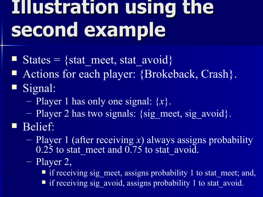
States = {stat_meet, stat_avoid}



Actions for each player: {Brokeback, Crash}.



Signal:

– Player 1 has only one signal: {x}.

– Player 2 has two signals: {sig_meet, sig_avoid}.



Belief:

– Player 1 (after receiving x) always assigns probability

0.25 to stat_meet and 0.75 to stat_avoid.

– Player 2,



if receiving sig_meet, assigns probability 1 to stat_meet; and,



if receiving sig_avoid, assigns probability 1 to stat_avoid.

Two states

Two states



Payoffs

B

C

B 2,1 0,0

C 0,0 1,2

B

C

B 2,0

0,2

C 0,1

1,0

Two signals of player 2

Two signals of player 2

B

C

B 2,1 0,0

C 0,0 1,2

B

C

B 2,0 0,2

C 0,1 1,0

If she receives sig_meet, then

Pr[stat_meet] = 1 and

Pr[stat_avoid] = 0.

If she receives sig_avoid, then

Pr[stat_avoid] = 1 and

States versus signals

States versus signals



Each state corresponds to a game.



Each signal for a player corresponds to a type of

the player.



When a player receives a signal, she believes in a

particular probability distribution over the states.

– The distribution describes the belief of the

corresponding type of player about the distributions

of the games.

Nash equilibrium

Nash equilibrium

A Nash equilibrium of a Bayesian game is a Nash equilibrium for the

strategic game for

P

_i

jT

_i

j players, in which the payo®for the i-th

player of type t

_i

with respect to action a is

X

! 2

Pr(! j t

_i

) ¢u

i

((a

i

; ^

a

¡ i

(! )); ! );

Notation

Notation

F

a

_i

, which has to be a member of A

_i

, is the action of the i-th

player speci¯ed in a.

F

u

_i

(¢;! ) is the pay-o®for the i-th player for state ! .

F

¿

_j

(! ) is the type (i.e., signal) of the j -th player corresponds to

state ! . Note that ¿

_j

is a function from

to T

_j

, which could

be many-to-one.

F

a

^

_j

_{= a(j ;¿}

_j

(! )) is the action of the j -th player of type ¿

_j

(! )

that is speci¯ed in action a.

F

a

^

_{¡ i}

_{= (^}

a

₁

; ^

a

₂

;:::; ^

a

_{i ¡ 1}

; ^

a

_{i +1}

; ^

a

_{i +2}

;:::; ^

a

_n

).

F

Pr(! j t

_i

) is the belief of the i-th player of type t

_i

about the

distribution of .

More information may

More information may

hurt…

hurt…

Two players, two states

Two players, two states

L

M

R

T 1, 0.5 1, 0 1, 0.75

B 2, 2 0, 0

0, 3

L

M

R

T 1, 0.5 1, 0.75 1, 0

B 2, 2

0, 3

0, 0

The setting

The setting



States = {stat_left, stat_right}



Actions for player 1: {T, B}.



Actions for player 2: {L, M, R}



Signals:

– Player 1 has only one signal: {sig_p1}.

– Player 2 has only one signal: {sig_p2}.



Belief:

– Player 1 (after receiving sig_p1) always assigns probability 0.5

to stat_left and 0.5 to stat_right

– Player 2 (after receiving sig_p2) always assigns probability 0.5

to stat_left and 0.5 to stat_right.

Player 1’s viewpoint

Player 1’s viewpoint

L

M

R

T 1, 0.5 1, 0 1, 0.75

B 2, 2 0, 0

0, 3

L

M

R

T 1, 0.5 1, 0.75 1, 0

B 2, 2

0, 3

0, 0

Each player assign probability 0.5 to each state.

L

M

R

T

1

1

1

Player 2’s viewpoint

Player 2’s viewpoint

L

M

R

T 1, 0.5 1, 0 1, 0.75

B 2, 2 0, 0

0, 3

L

M

R

T 1, 0.5 1, 0.75 1, 0

B 2, 2

0, 3

0, 0

Each player assign probability 0.5 to each state.

L

M

R

T 0.5

0.375

0.375

The Nash equilibrium

The Nash equilibrium

L

M

R

T 1, 0.5 1, 0 1, 0.75

B 2, 2 0, 0

0, 3

L

M

R

T 1, 0.5 1, 0.75 1, 0

B 2, 2

0, 3

0, 0

Each player assign probability 0.5 to each state.

L

M

R

T 1, 0.5 1, 0.375 1, 0.375

B 2, 2

0, 1.5

0, 1.5

Information

Information



The original setting is like both players

have “no information” about the

distribution of the game.



What if player 2 knows that the game they

are playing is the left one?

Player 1’s viewpoint

Player 1’s viewpoint

L

M

R

T 1, 0.5 1, 0 1, 0.75

B 2, 2 0, 0

0, 3

L

M

R

T 1, 0.5 1, 0.75 1, 0

B 2, 2

0, 3

0, 0

L

M

R

T

1

1

1

B

2

0

0

Prob.

= 0.5

Prob.

= 0.5

Player 2’s viewpoint

Player 2’s viewpoint

L

M

R

T 1, 0.5 1, 0 1, 0.75

B 2, 2 0, 0

0, 3

L

M

R

T 1, 0.5 1, 0.75 1, 0

B 2, 2

0, 3

0, 0

L

M

R

T 0.5

0

0.75

B

2

0

3

Prob. = 1

Prob. = 0

The Nash equilibrium

The Nash equilibrium

L

M

R

T 1, 0.5 1, 0 1, 0.75

B 2, 2 0, 0

0, 3

L

M

R

T 1, 0.5 1, 0.75 1, 0

B 2, 2

0, 3

0, 0

L

M

R

T 1, 0.5

1, 0

1, 0.75

B 2, 2

0, 0

0, 3

Prob. = 1

Prob. = 0

Prob.

= 0.5

Prob.

= 0.5

Similarly, if player 2 is told that

Similarly, if player 2 is told that

they are playing the right

they are playing the right

game...

game...

L

M

R

T 1, 0.5 1, 0 1, 0.75

B 2, 2 0, 0

0, 3

L

M

R

T 1, 0.5 1, 0.75 1, 0

B 2, 2

0, 3

0, 0

L

M

R

T 1, 0.5 1, 0.75

1, 0.

B 2, 2

0, 3

0, 0

Prob. = 0

Prob. = 1

Prob.

= 0.5

Prob.

= 0.5

More information may

More information may

hurt…

hurt…

應同學要求

應同學要求

舉一個 signals 與 states 間之對

應關係稍微複雜一點的例子

Brokeback or Crash

Brokeback or Crash



Belief of Player 1, who prefers B to C.

– with probability 1/2 player 2 wants to go to movie together, and

– with probability 1/2 player 2 does not want to go to movie

together.



Belief of Player 2, who prefers C to B.

– with probability 2/3 player 1 wants to go to movie together, and

– with probability 1/3 player 1 does not want to go to movie

together.



Each player knows whether or not herself wants to go to

yy B

C

B 2,1 0,0

C 0,0 1,2

yn B

C

B 2,0 0,2

C 0,1 1,0

ny B

C

B 0,1 2,0

C 1,0 0,2

nn B

C

B 0,0 2,2

C 1,1 0,0

player 1

想一起去

player 1

不想一起去

player 2

想一起去

player 2

不想一起去

1/2

1/2

1/2

1/2

2/3

2/3

1/3

1/3

yy B

C

B 2,1 0,0

C 0,0 1,2

yn B

C

B 2,0 0,2

C 0,1 1,0

ny B

C

B 0,1 2,0

C 1,0 0,2

nn B

C

B 0,0 2,2

C 1,1 0,0

player 1

想一起去

player 1

不想一起去

player 2

想一起去

player 2

不想一起去

1/2

1/2

1/2

1/2

2/3

2/3

1/3

1/3

States and signals

States and signals

F

_{State space = f yy;yn;ny;nng.}

F

Signals (i.e., types)

I

T

= f y

;n

g.

I

T

= f y

;n

g.

F

Mapping

I

¿

(yy) = ¿

(yn) = y

and ¿

(ny) = ¿

(nn) = n

.

I

¿

(yy) = ¿

(ny) = y

and ¿

(yn) = ¿

(nn) = n

.

F

Belief

I

Pr(yy j y

) = Pr(yn j y

) = 0:5 and Pr(ny j y

) = Pr(nn j y

) = 0.

I

Pr(yy j n

) = Pr(yn j n

) = 0 and Pr(ny j n

) = Pr(nn j n

) = 0:5.

I

Pr(yy j y

) = 2=3, Pr(ny j y

) = 1=3, and Pr(yn j y

) = Pr(nn j y

) = 0.

E.g., Player 1’s expected payoff

E.g., Player 1’s expected payoff

The expected payo®of player 1 of type y

₁

, if player 1 chooses B and

player 2 chooses (B;C) (i.e., a = (B;(B;C))), is

X

! 2

Pr(! j y

₁

) ¢u

₁

((B;a(2;¿

₂

(! )));! )

= 0:5¢(u

1

((B;a(2;¿

2

(yy)));yy) + u

1

((B;a(2;¿

2

(yn)));yn)) +

0¢(u

1

((B;a(2;¿

2

(ny)));ny) + u

1

((B;a(2;¿

2

(nn)));nn))

= 0:5¢(u

1

((B;a(2;y

2

));yy) + u

1

((B;a(2;n

2

));yn))

= 0:5¢(u

1

((B;B);yy) + u

1

((B;C);yn))

= 0:5¢(2+ 0)

= 1:

Therefore, we have

Therefore, we have

Player 1 (B, B) (B, C) (C, B) (C, C)

B

1

E.g., Player 2’s expected payoff

E.g., Player 2’s expected payoff

T heexpected payo®of player 2 of typen

₂

, if player 1 chooses (C;B ) and player

2 chooses C (i.e., a = ((C;B);C)), is

X

! 2

Pr(! j n

₂

) ¢u

₂

((a(1;¿

₁

(! )); C);! )

=

2

₃

¢u

2

((a(1;¿

1

(yn));C); yn) +

1

₃

¢u

2

((a(1;¿

1

(nn));C);nn) +

0¢(u

₂

((a(2; ¿

₁

(ny));C);ny) + u

₂

((a(2;¿

₁

(yy)); C);yy))

=

2

₃

¢u

2

((a(1;y

1

);C);yn) +

1

₃

¢u

2

((a(1;n

1

);C);nn)

=

2

₃

¢u

2

((C; C);yn) +

1

₃

¢u

2

((B ;C);nn)

=

2

₃

¢0+

1

₃

¢2

=

2

₃

:

Therefore, we have

Therefore, we have

Player 2

B

C

(B, B)

(B, C)

(C, B)

2/3

(C, C)