國
立
交
通
大
學
財務金融研究所
碩
士
論
文
從行為財務觀點探討超額股票報酬及經濟附加價值
間的關係
The Relationship between Excess Stock Return and EVA from the
Behavioral Finance Perspective
研 究 生: 陳英茵
指導教授: 王淑芬 博士
從行為財務觀點探討超額股票報酬及經濟附加價值間的關係
The Relationship between Excess Stock Return and EVA from the
Behavioral Finance Perspective
研 究 生:陳英茵 Student:Ying-Yin Chen
指導教授:王淑芬 博士 Advisor:Dr. Sue-Fung Wang
國 立 交 通 大 學
財務金融研究所
碩 士 論 文
A Thesis
Submitted to Graduate Institute of Finance College of Management
National Chiao Tung University in partial Fulfillment of the Requirements
for the Degree of Master in Finance
June 2011
Hsinchu, Taiwan, Republic of China
從行為財務觀點探討超額股票報酬及經濟附加價值間的關係
研 究 生:陳英茵
指導教授: 王淑芬 博士
國立交通大學財務金融研究所碩士班
摘要
效率市場假說與行為財務學的觀點對於市場的資訊反應有所不同,前者認為企業經 營資訊會充分反映在股價報酬,而後者則認為股價報酬具有先行性之資訊效果。從過 去的文獻發現企業的每股盈餘(EPS)在效率市場假說之下的資訊含量比較高, 然而在 2002 年行為財務學的崛起,發現企業的獲利行為與市場的表現並不完全一致。文獻上 對於 EPS 與經濟附加價值(EVA)何者具有較高的資訊含量一直沒有定論。有鑑於此,本 研究以美國市場的製造業為樣本進行實證研究,並以股價報酬與兩種超額股價報酬的 代理變數分別利用縱橫資料迴歸(Panel 迴歸)都發現 EVA 對這三種股票報酬的資訊內 涵較 EPS 高,並進一步透過因果關係模型分析,其結果發現 EPS、EVA 都與股票報酬間 呈現反向因果關係,尤其 EVA 相對更為顯著,此符合行為財務學的論點。 關鍵字:行為財務、因果分析、經濟附加價值The Relationship between Excess Stock Return and EVA from the Behavioral
Finance Perspective
Student:Ying-Yin Chen Advisor: Dr. Sue-Fung Wang
Graduate Institute of Finance
National Chiao Tung University
ABSTRACT
Efficient market hypothesis (EMH) and behavioral finance have different point of views on the market’s reaction to information. The former believes that business operating information is fully reflected in stock returns, whereas the latter states that stock returns have price leadership over business information. Previous literature shows that earnings per share (EPS) is more informative under EMH; however, after the blooming of behavioral finance in 2002, recent research has shown that corporate operating profitability is not at all consistent with the market perception. Literature has not been conclusive on relative information content for EPS and EVA. This study explores the empirical data of manufacturing firms within the US market. Total stock returns and two excess stock returns are first used as proxies through panel regression analysis, respectively. Results show that EVA is more informative than EPS for all three stock returns. Furthermore, a causality test in performed, revealing that both EVA and EPS present reverse causalities to the three stock returns, and EVA is relatively more significant. These results are consistent with the perspective of behavioral finance.
誌謝
努力了將近一年多的時間,論文的工作終於來到了尾聲,真的要感謝很多人的幫 助。首先要感謝我的指導教授王淑芬老師,在這段時間內對我的論文的大方向指導, 尤其是關於財務觀念的清楚說明,使得缺乏相關背景的我,可以比較容易的抓住研究 的方向;以及老師在每一次討論會議中,對我的文章編寫或是報告方式所做的建議。 特別感謝幾位口試委員不辭辛勞的幫忙審核論文和給出的改進建議。 另外,自然要特別感謝我的家人們,在論文的工作中經常必須面臨晚歸以及通勤 的狀況,多虧她們的體貼與關懷,每天外帶的家常便當,忙裡偷閒的喝茶時間,使得 我可以持續地堅持下去。最後,還要感謝眾多研究室同學的鼎力相助:感謝吳堃瑋同 學在計量模型方法以及文書處理格式的繁雜問題裡給我的許多幫助;感謝吳思蓉學姊 在搜尋資料庫的時候所給的額外幫忙;感謝同一研究室的黃光萍、黃馨儀和其他同學 們,在辦公室討論時所給的很多很多相關文獻或是模型設計的建議。 真的要再次謝謝各位對我的學位論文所給的幫助! 陳英茵謹製 國立交通大學財務金融所碩士班 中華民國一百年六月List of Contents
摘要 ... i ABSTRACT ... ii 誌謝 ... iii List of Contents ... iv List of Tables ... v 1. Introduction ... 1 2. Methodology ... 52.1. Data and Variable Definition ... 5
2.2. Models and Hypotheses ... 12
(1) Whole sample model ... 12
(2) Sub-period model ... 13
(3) Causality model ... 13
2.3. Beta Estimation ... 15
3. Regression Results ... 16
3.1. Whole Period Model ... 16
3.2. Sub-period Model ... 21
3.3. Causality Model ... 23
3.4. Robustness Check ... 25
4. Conclusion ... 29
List of Tables
Table 1 Definitions of Key Variables ... 6
Table 2 Summary Statistics of Key Variables ... 9
Table 3 Panel Regression — Whole Sample Model for EPS ... 17
Table 4 Panel Regression — Whole Sample Model for EVA ... 19
Table 5 Panel Regression -Sub-period Model ... 22
Table 6 Two-way Granger Causality and Wald Test ... 24
Table 7 Panel Regression – Sub-period Model Adjusted by Clustered Robust Standard Errors ... 26
1. Introduction
“A company's market value is a function of its book value of equity, earnings, and other information” (Ohlson, 1995). One can either interpret firm value as the risk premium explained by common market risk factors in asset pricing theory (Fama & French,
1996–2008; Ali, Hwang, & Trombley, 2003; Baginski & Wahlen, 2003). Alternately, firm value can also refer to operating performance based on summation of accounting numbers in fundamental analysis (Ohlson, 1995; Myers, 1999). Although performance sometimes fails to be realized as market stock price, the reason business valuation from market and operating perspectives is too distinct remains unexplained.
No one knows the intrinsic value of firms under efficient market hypothesis (EMH). Scholars believe market stock price to be the best reflection of intrinsic value. We can thus evaluate the degree of asymmetric information through the explanatory power of valuation indicators to market stock price in relative magnitude of adjusted R-square or correlation coefficients (Yoo et al., 2004; 2008). Most studies often focus on one question: “Which valuation indicator is more informative due to lower asymmetric information?” In the present paper, we employ three market stock returns (Ri, ER1, and ER2) as proxies for performance from the market perspective (Fama & French, 1998–2008; Bhagat & Bolton, 2008). In addition, we use two earning-based measures, EPS and EVA1
The pros and cons of EPS have been well documented in many studies and textbooks (Ross, 2006). EPS is considered as the shareholders’ wealth, and more reasonably related to
, as proxies for valuations from the operating perspective to illustrate the information content between EPS and EVA.
1
EVA (economic value added) is also known as residual earning or residual income (RE or RI). Basic formula of EVA in per share basis (1) is listed below:
EVA t = EPS t - r × BPS t-1 , where EPS t denotes forecasted EPS at time t-1; r denotes Implied
the goal of maximizing firm value. Thus, EPS is considered more highly associated with both returns and firm values than EVA or cash flow from operations (Biddle, Bowen, &Wallace, 1997). In addition, because the computation of EVA contains EPS, the
shortcoming of EPS is passed on to EVA as well (Ohlson, 2000). Major problems of EVA can be demonstrated by its basic formula in per share basis in notation 1.
The first problem is forecast EPS. Although forecast EPS is not available at all times in all firms, some researchers prefer to articulate the role of forward EPS in valuation. They state that forward EPS is more informative than EPS, EVA, DCF, and DDM (the worst is listed last) (Ohlson & Juettner-Nauroth, 2000). Meanwhile, according to Richardson and Tinaikar (2004), there exist detective links between historical and forecast data branches, which often produce similar results. Moreover, long-term analyst earning forecasts into EVA have been proven not to improve pricing performance significantly (Lo & Lys, 2001). Some, such as Frankel and Lee (1999), continue to use shorter forecast horizon with one- and two-year ahead analyst earnings forecasts; however, these still suffer from biases in forecasting errors. The limitations encountered by previous studies suggest the validity of using historical EPS over forecast EPS in this paper. The second problem with EVA concerns ICOE2. ICOE must be estimated, and is often viewed exogenous. In the present study, we use CAPM-derived ICOE because individual betas predict positive and
systematic association to ICOE in the literature (Yoo et al., 2004)3
2 ICOE here is derived from CAPM, which substitutes beta for individual firms (βi) in models because
individual betas predict positive and systematic association to ICOE in literature. Several alternative approaches to estimate ICOE are well reviewed in Section 2.1 of Yoo et al. (2004).
. Likewise, we obtain CAPM-derived ICOE by substituting beta for individual firms (βi) into CAPM. The third problem with EVA involves clean surplus relation (CSR) violation. According to Ohlson
3 Several alternative approaches to estimate ICOE are well reviewed in Section 2.1 of Yoo et al. (2004): (1)
ex post realized stock returns as natural proxy for the ex ante ICOE, but proven noisy and potentially biased (Fama & French, 1997; Elton, 1999); (and 2) internal rate of return (IRR) that equates stock prices with the valuations based on analyst earnings forecasts (Gebhardt et al., 2001).
Most variation of stock returns can be described by FF3 or FF4 (above 80% in US market), however, stock returns prove to be noisy; thus, we neglect FF4-derived ICOE.
(2000), CSR violation could affect EVA on a case-by-case basis.
Despite problems of EVA above, some studies continue to align with EVA to be more informative. Frankel and Lee (1999) conclude that firm value estimates derived from EVA can better explain the cross-sectional distribution of the stock prices, accounting for more than 70% of its variation within 20 countries, than earnings or book value. Even for studies that claim EPS outperforms EVA, empirical results continue to reveal that EVA has
significant marginal contribution (Biddle, Bowen, & Wallace, 1997; Lundholm, 2001; Yoo et al., 2004; 2008)4. Therefore, EVA has information unique from EPS. In addition, the authors suggest that EVA and AEG (abnormal earning growth) models are more related to systematic and industrial impact and risks (Jeon, Kang, & Lee, 2003, 2005; Cheng, 2004; Baginski & Wahlen, 2003). Yoo et al. (2004; 2008) indicate that these risks possibly represent economic-wide and country-level, industry-specific5
In sum, early studies all show that EPS is more informative (Biddle, Bowen, & Wallace, 1997; Ohlson & Juettner-Nauroth, 2000). However, a phenomenon of conflict results on information content is evident approximately after year 2000. Recent studies show that EVA is more informative otherwise (Frankel & Lee, 1999; Yoo et al., 2004, 2008). The cause of such changes in the results remains unknown.
related information. Some suggest EVA may be more sensitive to ICOE because of its inner beta estimation in the hotel business; however, there is a lack of significant empirical results. We argue that EVA can reflect some information from the market.
Because of the coincidence of time with conflict in studies involving EVA, we consider whether this can be caused by the rising angle of behavior finance. Behavior finance provides a fresh viewpoint to review many issues, especially in light of Kahneman’s
4 Biddle, Bowen, and Wallace (1997), using incremental tests, suggest that EVA components can add
marginally to information content beyond earnings. Lundholm (2001) suggests that, under certain assumptions, DCF and EVA can even carry similar information. Yoo et al. (2004, 2008) list facts regarding uncertain dominance of EVA depending on clean surplus relation (CSR) in global case.
5 Gode and Mohanram (2003) and Guay, Kothari, and Shu (2003) claim ICOEs derived from EVA (RIV
Nobel Prize in 2002. Kahneman’s study is more committed to ideas regarding psychology such as anticipation, bias of analysts, and mental account (Tversky & Kahneman, 1981; Thaler, 1985). The studies on behavior finance prove to against the impact of EMH-based studies. In the present study, we aim to determine whether behavioral finance effect also affects our valuation.
To be more specific, in business valuation, EMH and behavioral finance have different point of views regarding market reaction. EMH believes business operating information is fully reflected in stock returns, whereas behavioral finance state stock returns have
leadership in business information over EMH. Therefore, some studies suggest behavioral finance effect is likely to have power for reversing the directions of causality between stock returns and earnings (Bar-Yosef, Callen, & Livnat, 1987; Peiers, 1997; Linnainmaa, 2010). This can be realized by dot-com companies during Internet bubbles. For companies such as America Online and Twitter, which have encountered long-time losses but still receive high market prices6
As a result, this study mainly develops to answer three questions: First, as previous studies did, we want to verify which earning indicator makes asymmetric information decrease the most. Further, we want to investigate whether the blooming of behavior finance does make a changing viewpoint of century, and whether we can directly see the behavior finance effect in time and in causality. Finally, can we then document which
, or for corporate companies such as Netscape and Facebook, which have new business models and lack of accordance of past performance, the earning-based valuations seem to be off the hook to the stock returns; otherwise, even though valuations are affected by stock returns, they do not correspond to the positive relationship between earnings and returns that we expect under EMH.
6 In the Internet bubble in 1998 to 2000, as Penman (2010) states, all dot-com companies worth over 1 trillion
dollars in total, with 33 times on average price-to sales ratio far beyond the historical level of 1, maintain only 30 billion dollars on revenue; a recent report by The Guardian UK (2011)) also suggests a 2nd phenomenon of Internet bubble may occur. Microblogger and Twitter have an estimated worth of $ 10 B; Facebook, which have recently planned to initiate IPO, is estimated to be worth $ 60 B; this figure is slightly over Ford ($ 55 B) and below Visa ($ 63 B).
earning indicator is more influenced by behavior finance effect, and thus affecting its information content.
Several firm characteristics, including financial constraints, growth of investments, profitability, solvency, and debt ratio, are viewed as control variables. These variables are not Fama and French factors, but are also recognized as existing influences on firm value in extensive prior studies7
The remainder of this paper is organized as follows. Section 2 describes the methodology, including the sample selection, research models, and beta estimations. Section 3 presents and discusses the empirical results. Section 4 provides a summary of our main findings and the conclusion.
. Some studies show that the information regarding these influences may not be possibly explained by FF factors. We specifically intend to sort out the impact of financial constraints (proxy by asset tangibility) on firm value, thereby showing that investing behavior changes under financial constraints.
2. Methodology
2.1. Data and Variable Definition
The sample consists of manufacturing firms (those with SIC codes between 2000 and 3999) of S&P 500 Index members (COMPUSTAT auto-selection in 2010) over the 1994 to 2009 period. Sample selection criteria also include panel data requirements, 1% data trimming of outliers, and at least 24–60 month-ahead CRSP stock returns available for individual firm’s beta estimation8. In all, 110 sample firms for 16 years of effective sample period remain.
7 The detailed discussion is provided in Section 2.1.
8 In the following, two parts are needed to estimate betas for individual firm (denoted as β
i): the computation of ICOE (denoted as r) based on CAPM, and the computation of expected stock returns (E(Ri)) based on FF4. Details are listed in Section 2.3 beta estimation.
Financial statement and accounting data for main variables such as EPS, book value of total assets, and number of shares are collected from COMPUSTAT and Global Vantage. Stock return data are available and computed from CRSP. Risk-free rate and Fama and French factors (MKT, SMB, HML, and MOM) are collected from the Kenneth R. French Data Library in Dartmouth website.
All key variables are defined in Table 1.
Table 1 Definitions of Key Variables
This table displays the definition of all key variables. The full sample period is from 1994 to 2009.9
Indication Variables Name of Variables Definition Proxy for Firm Value10 Stock Return (FV)
Ri Annual stock return computed from CRSP
Annual Excess Return (1)
ER1 Annual stock return – Risk-free rate
= Sum of 12-month (Stock return – T-bill rate)
Annual Excess Return (2)
ER2 Annual stock return – Expected stock return derived from FF411
Measures of Valuations (V)
Actual EPS EPS (Income before extraordinary items-Preferred dividends) / Common shares outstanding
Economic Value Added (per share)
EVA EVA t (per share)
= Earnings per share at time t 12– Implied cost of equity13
= EPS t – r × BPS t-1
× Book value of common equity per share at time t-1
9 Most definition of our control variables follow Hahn and Lee (2009) and other reference we already
mentioned in paper, including I, P, and G…,etc, whose original description can be referred to Hahn and Lee (2009) P.898-904 and Appendix P.919, and the detail is listed in our Table 1.
Definition of stock returns and EVA related variables mainly follow Fama, French ,1998-2008 and Yoo et al., 2004,2008, and there are some time adjustments concerning financial data publish in accounting system are considered here but omitted in time line description. The original description can be referred to their notations, and the detail is listed in our Table 1 as well.
10
In general discussion, extensive literature use stock returns (denoted as Ri), Tobin’s Q, and ROA as proxies for firm value or firm performance in solid and regular illustration in textbook of finance. Stock returns should to be considered of equity value because of the return in market value of holding a share of equity.
11
Two kinds of expected stock returns (denoted as E(Ri)) are considered in this paper: risk-free rate and expected return derived from FF4.
12We use actual earning at time t as the forecasted ahead earning of time t-1. The implication is that we use
forecasts exactly equal to actual.
13
Proxy for
Financial constraints (FC)
Size ln(TA) The natural log of book value of total assets at fiscal year end.
Tangibility1 Tang1 Cash holdings + 0.715 × Receivables + 0.547 × Inventories + 0.535 × PPE) / book value of total assets14
Tangibility2 Tang2 Cash holdings + 0.715 × Receivables + 0.547 × Inventories + 0.535 × PPE - book value of total debt) / book value of total assets
Proxy for Profitability (P)
Profitability Profitability (P)
EBITDA/ Book value of total assets
Proxy for Growth of Investments (G)
Investment Investment (I)
Capital expenditures / Beginning-of-period capital stock
= CAPEX / lagged PPE(lagged property, plant, and equipment)
Tobin’s Q Q Market value of total assets / Book value of total assets
= Book value of total assets + Market value of common shares - Book value of common shares + Deferred tax ) / Book value of total assets
Proxy for Solvency(S)
Current Ratio CR Current assets/ Current liability
Proxy for Debt Ratio(D)
Times Interest Earned
TIE Times Interest Earned (or Interest coverage ) = Operating income before depreciation / Interest expense
Debt Ratio DR Debt ratio (or Book leverage)
= (Book value of Short-term debt + Long-term debt ) / Book value of equity
Three stock return measures are used as dependent variables (Ri, ER1, ER2). They also represent the valuation made from market perspective. In the literature, stock returns are decomposed into expected (or normal) returns and excess (or abnormal) returns. However,
14 The weights of each item in tangibility follow those suggested by Almeida and Campello (2007) and Hahn
in this paper, the first expected return is equal to risk-free rate and the second expected return is mostly constructed as benchmark for the four-factor model (hereafter, FF4) of Fama and French, which is adapted from the regression procedures of Fama and MacBeth (1973). Annual stock return is the proxy for total value, and two excess stock returns are the proxies for excess value. Because of this difference of meanings, we expect to observe distinct empirical results when different dependent variables are used.
Two earning-based valuation indicators are used as major independent variables (EPS and EVA). They also represent the valuation made from operating perspective composed of accounting numbers. EPS is commonly considered as the measure of total equity value, and reflects much more on absolute performance, indicating the absolute magnitude of profit per share. Therefore, we infer that EPS might be more associated with stock returns (Ri). Meanwhile, EVA is equal to the remaining part of EPS minus the total opportunity cost of equity funds. That is, EVA should be considered as an excess equity value. Moreover, EVA originally reflects on relative performance, indicating excess profit earned comparing to the growth with cost, thus it should indicate excess returns (ER) more adequately.
EVA decomposes EPS into normal value and excess value, where normal value is concerned with ICOE, whereas excess value is simply EVA. Using the decomposition of EPS, we want to explore whether we can augment the goal of finance to a further step. That is, we can maximize firm value by maximizing shareholder wealth. Nevertheless, can we can maximize shareholder wealth by maximizing EVA because another part of EPS is only of normal value. If this value is true, maximization of firm value is then more reasonably related to the maximization of EVA.
Several firm characteristics are reported in this paper, including financial constraints, growth of investments, profitability, solvency, and debt ratio, are viewed as control variables. We attempt to develop the expected signs of coefficients of those variables in the following discussion, and we provide descriptive statistics for key variables in Table 2.
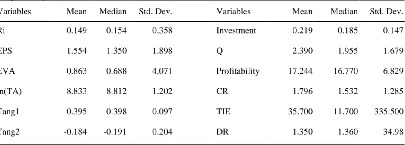
Table 2 Summary Statistics of Key Variables
This table displays the summary statistics of key variables reported as time-series averages of the
cross-sectional mean, median, and standard deviations over the period from 1994 to 2009. The number of total sample firm years (N) is 1760.
Variables Mean Median Std. Dev. Variables Mean Median Std. Dev.
Ri 0.149 0.154 0.358 Investment 0.219 0.185 0.147 EPS 1.554 1.350 1.898 Q 2.390 1.955 1.679 EVA 0.863 0.688 4.071 Profitability 17.244 16.770 6.829 ln(TA) 8.833 8.812 1.202 CR 1.796 1.532 1.285 Tang1 0.395 0.398 0.097 TIE 35.700 11.700 335.500 Tang2 -0.184 -0.191 0.204 DR 1.350 1.360 34.98
In Table 2, EVA is accounted for as 55.5% of EPS on average (0.863/1.554), but with larger variance (4.071 > 1.898). This indicates that a few firms earn abnormally. Although Ri, EPS, and EVA are positive in mean, they still present negative relation to Ri in some cases afterward. Two measures of asset tangibility have counter signs in mean due to definitions. Thus, the ratio of total debt to total assets of book value on average is approximately 57.9% [0.395-(-0.184)].
Before we proceed with our discussion regarding expected signs of coefficients of variables, we must point out that collinearityproblems15
15
In multivariate analysis, the existence of collinearity may cause noise on coefficients of variables. And for some variables here, high correlations exist between y and x, and x and x. General procedure to deal with collinearity, such as observing Pearson correlation table and setting up partition of variables suggested in literatures, are considered in this study. We also consider endogenous problem, which will be mentioned in Section 3.4 Robustness check.
exist in our model (such as Q to Ri, profitability (P) and investment (I), the correlation is approximately 30% and 50%, respectively). Based on our partition of variables, collinearityexists between stock returns, investments, Tobin’s Q, and profitability (P is the ratio of EBITDA to book value of total assets, and can be interpreted as cash-based ROA) (Aggarwal & Kyaw, 2006). ROA can also be used to measure profitability. Previous studies usually classify investment and Tobin’s Q under growth opportunity of investments, and state that growth is realized as
future profitability; thus, at times, profitability and investments are classified as categories of profitability as well (Hahn & Lee, 2009; Tim & Vidhan, 2008; Doukas & John, 1995). However, stock returns, investments, Tobin’s Q, and ROA are all considered proxy variables for firm performance in a large body of literature (Klapper, 2004; Wright, Kroll, Mukherji, & Pettus, 2009; Bhagat & Bolton, 2008). We also attempt to make some adjustments in the following models by providing models without coexistence of stock returns, Tobin’s Q, and profitability; the results are mentioned, but are omitted from the final table to make the coefficients in empirical results more stable and reliable.
Expected signs of coefficients of variables
We use the natural log of a firm’s assets at the end of the year as the proxy of firm size (Gozzi et al., 2008)16
However, in some cases, asset size also serves as proxy for firm risk. When asset size is the proxy for firm risk, controversial results arise, as reflected in previous studies. Some studies claim that size has a positive effect on the risk taking of a firm due to the moral hazard associated with “too-big-to-fail” policy (Boyd, Jagannathan, & Kwak, 2009), whereas others suggest a negative correlation between firm size and risk (Fama & French, 1992). Thus, both positive and negative impacts on firm value caused by asset size seem plausible, if one views stock returns as risk premiums.
. Firm size is considered a determinant of financial constraints or capital market access (Titman & Wessels, 1988) that affects decisions of managers and firm value (Cho, 1998; Lee & Chuang, 2009). It is positively related to firm value (Opler & Titman, 1994;Maury, 2006) because small firms are younger and less well known, and are therefore more likely to face financing constraints and vulnerable to capital market imperfections arising from information asymmetries and collateral constraints (Gertler & Gilchrist, 1994).
16 Other proxy variables for firm size also exist, such as natural log of a firm’s total sale or market value of
Asset tangibility is considered the expected asset liquidation value for a firm. A firm with greater expected asset liquidation value (or collateral assets) should have less financial constraints, and therefore have a higher firm value (Almeida & Campello, 2007; Hahn & Lee, 2009). Following all that, we expect that financial constraints are negatively related to stock returns (measures of financial constraints are all reverse indicators; when these measures are bigger, financial constraints are less, and stock returns are bigger). We also expect that measures of financial constraints are positively related to stock returns.
The discussion of financial constraints in some studies often involves issues of maturity stage and firm scale. Previous studies suggest that large firms tend to have low growth (maturity stage) and lower firm performance (Opler &Titman, 1994;Maury, 2006; Lee & Chuang, 2009). If we attempt to restate the description above, we could say that large firms tend to earn normal stock returns and have lower firm value, whereas small firms tend to earn abnormal (or excess) stock returns and have higher firm value. Therefore, this theory suggests a negative relation of size to stock returns, and negative relation of size to excess stock returns.
In sum, after combining theories of size effect, firm risk, financial constraints, and maturity stage, both positive and negative impacts on firm value caused by asset size are still likely to appear, and the relation of asset tangibility to excess stock returns remains unknown as well.
Growth of investments and profitability both have positive contribution to firm value (Hahn & Lee, 2009, Fama & French, 1992), and naturally, we expect to observe a positive relation between investments, profitability, and stock returns. As Penman (2010) says, “Don't pay too much for the growth.” After considering corresponding opportunity cost of equity funds, seeking for growth of investment and profitability may be harmful to a corporation. That is, when firms make inefficient investments with rate of returns lower
than ICOE, we infer that such may enhance stock returns, while simultaneously decrease excess stock returns.
Current ratio is expected to observe a positive relation with stock returns (Menon,1987; Richards, 1980; Donaldson, 2000). Meanwhile, debt ratio (or book leverage) is expected to observe a negative relation with stock returns. Times interest earned is a quality measure for debt. Studies show controversial results on the relation between leverage and firm value; some support a positive relation (Harris & Raviv, 1990; Stulz, 1990), whereas others support a negative relation (Opler & Titman, 1994; Majumdar & Chhibber, 1999; Weill, 2008). Studies also suggest that the relation is based on degrees of growth opportunities; thus, debt financing will enhance firm value in low-growth firms, but reduce firm value in high-growth firms (McConnell & Servaes, 1995; Jung, Kim, & Stulz, 1996; Barclay, Marx, & Smith, 2003). Often, high debt ratio can reduce the opportunities of managers to overinvest, and decrease agency cost in low-growth firms, thereby generating high free cash flow (Jensen, 1986; Stulz, 1990; Gul & Tsui, 1998). Based on the pecking order theory, firms that are more profitable can meet the funding requirements through internal earnings and less borrowing (Myers & Majluf, 1984).
2.2. Models and Hypotheses
Three kinds of model designs are presented in this paper: whole sample model, sub-period model, and causality model.
(1) Whole sample model
In the whole sample model, we take a full effective sample period (1994–2009) to conduct panel regression tests with fixed effect and no intercept model settings. Based on our partition of control variables mentioned above, we proceed to determine the valuation indicator, EPS or EVA, that has better explanatory power of stock returns in all eight model combinations.
(2) Sub-period model
According to Haugen (1999), EMH-based studies and behavior finance are rivals in new finance period17
Therefore, in sub-period model, we set the year 2002 (the year the Nobel prize is won by Kahneman, a scholar of behavior finance) as the cut-off point of the rising stage of behavioral finance; thus, we divide the whole sample period into two sub-periods (i.e., the former period, 1994–2001, and the latter period, 2002–2009. The year 2009 is used as year dummy to avoid the influence of financial crisis). We then proceed to apply the same panel regression tests to each sub-period to compare their explanatory power. Under EMH, the explanatory power after considering FF factors should increase (Former < Latter). However, we expect to observe the “behavior finance effect” as time goes on; thus, we infer that the explanatory power of sub-period models will decrease over time (Former > Latter).
. Under this competition, we investigate whether the rising perspective of behavior finance seriously impact the power of EMH-based studies on business valuation.
(3) Causality model
We attempt to investigate the interactions between valuations made from operating and market perspectives, and test for the “behavioral finance effect” by causality models. We can consider the operating perspective consisting of two levels. Based on the theory of finance on value generators, major operating decisions (investing, financing, and payout policies) contribute to the quality of performance of a firm, and the performance reflect on valuations made from operating perspective such as EPS and EVA. As a result, we prepare to carry out the causality tests by setting up a three-step
17 According to Haugen 1(999), the present finance progress could be divided into several segmentations:
accounting-related research dominates “Old Finance” period until 1960; economic theories and rational hypothesis influence “Modern Finance”period until 1980. After 1980, theories regarding inefficiency and psychology take over, thus to form the “New Finance” period.
analysis on causality as follows: (I) investigate the causality between financial constraints and earnings from operating perspective; (II) investigate the causality between earnings from operating perspective and returns from market perspective; and (III) investigate the causality between financial constraints (FC) and returns from market perspective (MP)
Following this logic, we are able to establish a natural causality loop under EMH for this three-step analysis: financial constraints (FC) belongs to parts of operating decisions as the literature stated (Hahn & Lee, 2009), asset size can be regarded as an index of financing policy, and tangibility can also be treated as the bridge index between financing and investing policies through the use of net operating assets or collateral assets. Thus, we conduct the first step of natural causality loop: (I) financial constraints affect valuations from operating perspective. Thus, if firms publish good valuations from operating perspective to the public, good informative announcement based on accounting analysis should bring up the market price of individual stock, or market stock returns of individual stock. Therefore, we conduct the second step of natural causality loop: (II) valuations from operating perspective affect valuations from market perspective. Finally, combining (I) and (II), we obtain the third step of natural causality loop: (III) financial constraints affect valuations from market perspective. This is consistent with a number of studies documenting that corporate investment behavior arising from financial constraints are reflected in the stock returns (Hahn & Lee, 2009; Forbes, 2007; Whited & Wu, 2006) because the inability to borrow externally causes many firms to bypass attractive investment opportunities; it
influences the firm value (Campello et al., 2010; Cleary, 1999) based on internal fund assumption (Fazzari et al., 1988).
We conduct the two-way Granger Causality and Wald tests18
Hypothesis 1: EVA is more informative due to lower information asymmetry.
to illustrate the causality or leadership between stock returns, financial constraints, and earning-based valuations. We expect to detect the behavior finance effect by reversing the directions of causality. We establish one hypothesis for each model design. A total of three hypotheses are listed below:
Hypothesis 2: The explanatory power of Fama and French’s market risk factors
reduces over time due to the rising perspective of behavior finance (psychological and other factors).
Hypothesis 3: There exists a reverse causality relationship (behavioral finance effect)
between stock returns (valuation from market perspective), earning-based valuation (valuation from operating perspective), and financial constraints.
2.3. Beta Estimation
In the present paper, two parts are needed to estimate betas for individual firms
(denoted as βi): one is related to the computation of EVA, whereas the other is related to the
computation of expected returns (risk-adjusted returns). The former follows CAPM, whereas the latter follows the Fama and French four-factor model.
We follow the COMPUSTAT procedure for beta estimation of individual firms. The data is only traceable within five years of the present date. For data out of this range, we adapt the formula and steps set in the database using S&P 500 Index returns as market returns (Rm), risk-free rate (Rf), stock returns of each firms (Ri) in monthly data form, to
estimate current individual beta (βi). At least 24–60 previous observations are required to
meet the regression requirements. We then substitute individual beta (βi) into CAPM to
18 The causality model requires the two preliminary tests (unit root test and co-integration test) to be
conducted to check whether the variable is stationary and existing an economic equilibrium, and an optimal lag number in time series model be selected based on AIC or SIC. In this paper, the validity of these preliminary results is checked, but omitted in the final table, and we conduct those tests by SAS procedures (varmax). We must note that the causality test cannot identify the difference between causality and leadership in statistic.
obtain ICOE (ri) for individual firms19
In the following, we estimate the expected stock return by the procedures in (Hahn & Lee, 2009): estimating the Fama and French factor loadings (β' ik) for individual stock i
using monthly rolling regressions with a 60-month window every month requires at least 24 monthly return observations in a given window and substituting those betas into the model E(Ri)= Rit− Rf t− Σ{k=1~4} β'ik×Fkt (3)
to obtain expected stock returns, where Rit is stock return of firm i at time t, Rft is the
risk-free rate (T-bill rate) at time t, and Fkt denotes one of the Fama and French four-factor
loading (MKT, SMB, HML, and MOM). .
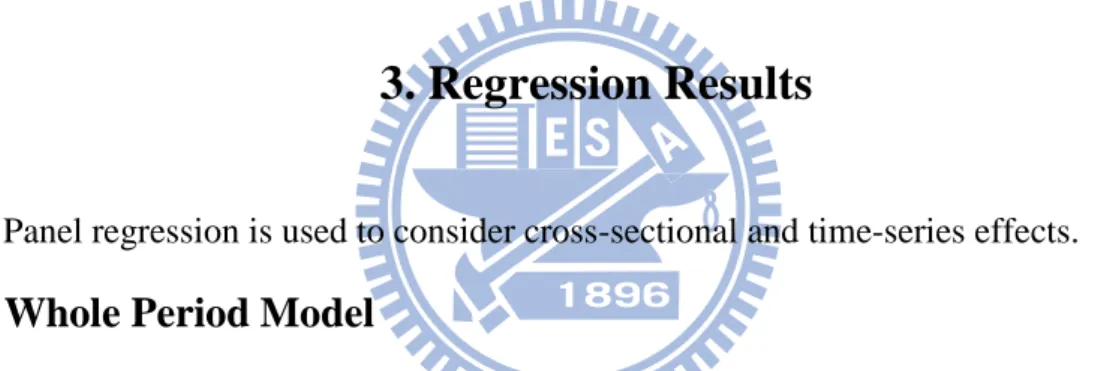
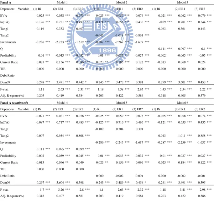
3. Regression Results
Panel regression is used to consider cross-sectional and time-series effects.
3.1. Whole Period Model
Table 3 and Table 4 report the panel regression results of the whole sample model for EPS and EVA. Several noticeable empirical results are significant, based on Tables 3 and 4. First, by comparing Table 3 and Table 4, we find that the explanatory power of EVA is
dominant over those of EPS in every model, (Average adj-R2:0.261 > 0.211,0.414 > 0.399, 0.583 > 0.560); therefore, it confirms H1: EVA is more informative due to lower
information asymmetry.
Furthermore, although EPS in Table 3 is positively related to total returns in
omitted-collinearity-adjusted models, EPS is not significant and negatively related with firm value, especially in some models whose dependent variable is stock return (Ri). This
19
CAPM derived ICOE (ri) = Rf +βi × [E(Rm) - Rf] (2);Industry betas (market value weightedβi
within a single industry ) for 19 industries (classified by SIC division) are once conducted; however, it does not seem to improve the empirical results. Therefore, it is omitted in the final table.
finding corresponds with prior studies claiming that EPS may be a misleading indicator of returns, likely because EPS can affect investment decisions due to earning management problems (Stern, 1974; Stewart & Jones, 2001)20
Second, we can observe the increasing explanatory power as we gradually change the dependent variable from stock return to excess return 2 (Average adj-R2:0.211 < 0.399 < 0.560;0.261 < 0.414 < 0.583). This finding illustrates the improvements made by adding Fama and French risk factors on valuation in the market perspective.
. In addition, this may illustrate some occasions in which valuations from operating and market perspective move in
counter-directions such as dot-com companies during Internet bubbles, which might encounter long-term loss on earnings but still receive high valuations and external funds from the market. In addition, as Table 4 shows, EVA is nearly negatively related to stock returns (Ri) in every case, suggesting that EVA may illustrate more behavioral finance effect.
Table 3 Panel Regression — Whole Sample Model for EPS
This table reports the regression coefficients but omits the associated t-statistics from the panel regression model with fixed effect and no intercept settings for whole sample period 1994 to 2009. The number of total sample firm-years (N) is 1760 for every model. F-statistics of validity tests of panel regression models are also provided. Three dependent variables, including stock returns, excess stock returns 1, and excess stock returns 2, are all used in each model, and earning-based valuation indicator EPS is used as the major independent variable. The table summarizes all model combinations composed of controlled variables: size, tangibility 1, tangibility 2, profitability, investment, Tobin’s Q, current ratio times interest earned, and debt ratio. (The detailed definition is listed in Table 1.) For example, Model 1 indicates three regression results conducted by three dependent variables explained by EPS as major independent variable plus first combinations of controlled variables in the model. *, **, and *** indicate significance at 10%, 5%, and 1%, respectively.
20 Some also suggest that the negative coefficients may due to long-run reversal condition of returns, because
Panel A Model 1 Model 2 Model 3
Dependent Variable (1) Ri (2) ER1 (3) ER2 (1) Ri (2) ER1 (3) ER2 (1) Ri (2) ER1 (3) ER2 EPS 0.014 ** 0.015 ** 0.039 * 0.014 ** 0.026 ** 0.048 ** 0.019 *** 0.017 *** 0.042 ** ln(TA) -0.197 *** 0.83 *** 0.62 *** -0.192 *** 0.738 *** 0.53 *** -0.156 *** 0.889 *** 0.663 *** Tang1 -0.128 0.353 0.463 -0.065 0.371 0.489 Tang2 -0.017 -1.198 -1.09 *** Investments -0.28 *** -2.273 *** -1.645 *** -0.28 *** -2.291 *** -1.669 *** Q 0.12 *** 0.076 *** 0.071 *** Profitability 0.003 -0.034 -0.024 *** 0.003 -0.029 -0.018 *** -0.01 *** -0.053 *** -0.039 *** Current Ratio 0.019 ** 0.163 ** 0.103 *** 0.019 * 0.197 * 0.135 *** -0.018 ** 0.081 ** 0.038 TIE 0.000 0.000 0.000 0.000 0.000 0.000 0.000 0.000 0.000 Debt Ratio Dum09 0.377 *** 3.166 *** 0.367 0.374 *** 3.177 *** 0.301 0.407 *** 3.272 *** 0.397 F-stat. 1.43 *** 2.9 *** 2.65 *** 1.6 *** 3.8 *** 3.5 *** 1.67 *** 2.79 *** 2.55 *** Adj. R-square(%) 0.143 0.404 0.562 0.143 0.408 0.565 0.28 0.389 0.555
Panel A (continued) Model 4 Model 5 Model 6
Dependent Variable (1) Ri (2) ER1 (3) ER2 (1) Ri (2) ER1 (3) ER2 (1) Ri (2) ER1 (3) ER2 EPS 0.019 *** 0.027 *** 0.05 ** 0.014 ** 0.018 ** 0.04 ** 0.014 ** 0.029 ** 0.049 ** ln(TA) -0.153 *** 0.799 *** 0.575 *** -0.197 *** 0.823 *** 0.618 *** -0.192 *** 0.732 *** 0.529 *** Tang1 -0.121 0.328 0.45 Tang2 -0.001 -1.15 -1.05 *** -0.018 -1.202 -1.09 *** Investments -0.278 *** -2.268 *** -1.644 *** -0.279 *** -2.286 *** -1.668 *** Q 0.12 *** 0.074 *** 0.071 *** Profitability -0.01 *** -0.048 *** -0.034 *** 0.003 -0.034 -0.024 *** 0.003 -0.029 -0.019 *** Current Ratio -0.018 ** 0.113 ** 0.069 ** 0.019 ** 0.163 ** 0.103 *** 0.019 * 0.196 * 0.135 *** TIE 0.000 0.000 0.000 Debt Ratio 0.000 -0.001 0.000 0.000 -0.001 0.000 Dum09 0.406 *** 3.284 *** 0.335 0.374 *** 3.178 *** 0.379 0.372 *** 3.188 *** 0.313 F-stat. 2.17 *** 3.65 *** 3.34 *** 1.43 *** 2.9 *** 2.67 *** 1.6 *** 3.82 *** 3.54 *** Adj. R-square(%) 0.28 0.393 0.558 0.143 0.405 0.562 0.142 0.409 0.565
Panel A (continued) Model 7 Model 8 Dependent Variable (1) Ri (2) ER1 (3) ER2 (1) Ri (2) ER1 (3) ER2 EPS 0.019 *** 0.02 *** 0.043 ** 0.019 *** 0.031 *** 0.052 ** ln(TA) -0.157 *** 0.882 *** 0.66 *** -0.153 *** 0.793 *** 0.573 *** Tang1 -0.063 0.335 0.468 Tang2 -0.001 -1.152 -1.05 *** Investments Q 0.12 *** 0.076 *** 0.071 *** 0.121 *** 0.074 *** 0.071 *** Profitability -0.01 *** -0.054 *** -0.039 *** -0.01 *** -0.049 *** -0.034 *** Current Ratio -0.018 ** 0.081 ** 0.038 -0.019 ** 0.112 ** 0.069 ** TIE Debt Ratio 0.000 -0.001 -0.001 0.000 -0.001 -0.001 Dum09 0.407 *** 3.288 *** 0.411 0.406 *** 3.299 *** 0.35
F-stat. 1.67 *** 2.78 *** 2.55 *** 2.17 *** 3.67 *** 3.37 *** Avg. . Avg. . Avg. Adj. R-square(%) 0.28 0.39 0.555 0.28 0.393 0.558 0.211 0.399 0.560
Table 4 Panel Regression — Whole Sample Model for EVA
This table reports the regression coefficients but omits the associated t-statistics from the panel regression model with fixed effect and no intercept settings for the whole sample period from 1994 to 2009. The number of total sample firm years (N) is 1760 for every model. F-statistics of validity tests of panel regression models are also provided. Three dependent variables, including stock returns, excess stock returns 1, and excess stock returns 2, are all used in each model, and earning-based valuation indicator EVA is used as the major independent variable. The table summarizes all model combinations composed of controlled variables: size, tangibility 1, tangibility 2, profitability, investment, Tobin’s Q, current ratio times interest earned, and debt ratio (the detailed definition is listed in Table 1.) For example, Model 1 indicates three regression results, which are conducted by three dependent variables explained by EVA as major independent variable plus the first combinations of controlled variables in the model.
*, **, and *** indicate significance at 10%, 5%, and 1%, respectively.
Panel A Model 1 Model 2 Model 3
Dependent Variable (1) Ri (2) ER1 (3) ER2 (1) Ri (2) ER1 (3) ER2 (1) Ri (2) ER1 (3) ER2 EVA -0.025 *** 0.058 *** 0.075 *** -0.025 *** 0.057 *** 0.074 *** -0.021 *** 0.062 *** 0.079 *** ln(TA) -0.126 *** 0.721 *** 0.497 *** -0.121 *** 0.656 *** 0.436 *** -0.09 *** 0.781 *** 0.544 *** Tang1 -0.119 0.333 0.407 -0.063 0.361 0.443 Tang2 -0.042 -1.018 *** -0.861 *** Investments -0.286 *** -2.253 *** -1.619 *** -0.287 *** -2.267 *** -1.639 *** Q 0.111 *** 0.097 *** 0.1 *** Profitability 0.01 *** -0.043 *** -0.032 *** 0.01 *** -0.037 *** -0.027 *** -0.002 -0.065 *** -0.05 *** Current Ratio 0.023 ** 0.156 *** 0.096 *** 0.023 ** 0.185 *** 0.122 *** -0.013 0.068 * 0.024 TIE 0.000 0.000 0.000 0.000 0.000 0.000 0.000 0.000 0.000 Debt Ratio Dum09 0.248 *** 3.471 *** 0.442 * 0.245 *** 3.473 *** 0.381 0.299 *** 3.601 *** 0.453 * F-stat. 1.11 2.63 *** 2.31 *** 1.18 3.38 *** 2.95 *** 1.43 *** 2.54 *** 2.22 *** Adj. R-square(%) 0.203 0.419 0.584 0.203 0.422 0.586 0.318 0.405 0.579
Panel A (continued) Model 4 Model 5 Model 6
Dependent Variable (1) Ri (2) ER1 (3) ER2 (1) Ri (2) ER1 (3) ER2 (1) Ri (2) ER1 (3) ER2 EVA -0.021 *** 0.061 *** 0.078 *** -0.025 *** 0.059 *** 0.075 *** -0.025 *** 0.058 *** 0.074 *** ln(TA) -0.087 *** 0.717 *** 0.483 *** -0.125 *** 0.716 *** 0.496 *** -0.121 *** 0.653 *** 0.435 *** Tang1 -0.109 0.304 0.394 Tang2 -0.007 -0.954 *** -0.808 *** -0.043 -1.011 *** -0.858 *** Investments -0.286 *** -2.245 *** -1.617 *** -0.287 *** -2.259 *** -1.637 *** Q 0.111 *** 0.095 *** 0.099 *** Profitability -0.002 -0.059 *** -0.045 *** 0.01 *** -0.043 *** -0.032 *** 0.01 *** -0.037 *** -0.027 *** Current Ratio -0.013 0.096 ** 0.049 0.023 ** 0.156 *** 0.096 *** 0.023 ** 0.184 *** 0.122 *** TIE 0.000 0.000 0.000 Debt Ratio 0.000 -0.002 -0.001 0.000 -0.002 -0.001 Dum09 0.297 *** 3.604 *** 0.398 0.243 *** 3.489 *** 0.456 * 0.241 *** 3.491 *** 0.395 F-stat. 1.7 *** 3.26 *** 2.8 *** 1.1 2.63 *** 2.32 *** 1.18 3.41 *** 2.98 *** Adj. R-square(%) 0.318 0.407 0.581 0.203 0.419 0.584 0.203 0.422 0.586
Panel A (continued) Model 7 Model 8 Dependent Variable (1) Ri (2) ER1 (3) ER2 (1) Ri (2) ER1 (3) ER2 EVA -0.021 *** 0.063 *** 0.08 *** -0.021 *** 0.062 *** 0.079 *** ln(TA) -0.09 *** 0.776 *** 0.542 *** -0.087 *** 0.715 *** 0.482 *** Tang1 -0.057 0.321 0.421 Tang2 -0.008 -0.946 *** -0.804 *** Investments Q 0.111 *** 0.097 *** 0.1 *** 0.111 *** 0.095 *** 0.099 *** Profitability -0.002 -0.065 *** -0.05 *** -0.002 -0.059 *** -0.045 *** Current Ratio -0.013 0.068 * 0.024 -0.013 0.096 ** 0.049 TIE Debt Ratio 0.000 -0.002 * -0.001 0.000 -0.002 * -0.001 Dum09 0.296 *** 3.623 *** 0.471 * 0.295 *** 3.625 *** 0.415
F-stat. 1.43 *** 2.54 *** 2.23 *** 1.7 *** 3.28 *** 2.82 *** Avg. Avg. Avg. Adj. R-square(%) 0.318 0.406 0.579 0.318 0.409 0.581 0.261 0.414 0.583
Third, we compare from the figures Table 3 to Table 4 and the expectation of variables in Section 2.2.
Coefficients of financial constraints are partly consistent with the expectation (Opler & Titman, 1994; Maury, 2006; Lee & Chuang, 2009); thus, significance is achieved. Among three measures for financial constraints (i.e., inverse measures), tangibility is positively related to stock returns, but negatively related to excess returns, whereas size is negatively related to stock returns and positively related to excess stock returns. These results may hint that small firms facing lower financial constraints tend to have higher stock returns, and large firms facing greater financial constraints tend to have more excess stock returns and vice versa, but we cannot conclude that strongly. Hahn & Lee, 2009 state that size effect cannot fully explain the difference created by financial constraints, even after considering FF factors. Even, in their study, they find that especially when under constraint-group (by lots of measures, such size, tangibility, bond rating…,etc), bigger tangibility is still more related to bigger excess returns significantly, and our results is similar to theirs.
Coefficients of growth of investments and profitability are not fully consistent with the expectation (Hahn & Lee, 2009; Fama & French, 1992). Significance is achieved in most cases, except in some models of Ri. Some models are negatively related to stock returns,
and even more negatively related to excess returns. This situation does not alter models avoiding collinearity. Possibly, for manufacturing firms in S&P 500 index members, firms making less investment tend to have higher stock returns. In addition, after considering corresponding opportunity cost of equity funds, firms making less investment tend to earn even higher excess stock returns.
On the one hand, coefficients of current ratio and debt ratio are mostly consistent with the expectation, although significance is only achieved with some models. On the other hand, this significantly improves models avoiding collinearity. Current ratio is positively related with stock returns (Menon, 1987; Richards, 1980; Donaldson, 2000), whereas debt ratio is negatively related with stock returns (Opler & Titman, 1994; Majumdar & Chhibber, 1999; Weill, 2008); however, times interest earned is not significant in all cases.
In sum, our empirical results illustrate that, for manufacturing firms in S&P 500 index members, small firms with less financial constraints, less investment, less profitability, higher current ratio, and less debt ratio tend to have significantly higher stock returns, whereas large firms facing greater financial constraints, less investments, less profitability, higher current ratio, and less debt ratio tend to have higher excess stock returns significantly.
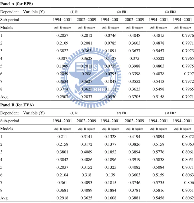
3.2. Sub-period Model
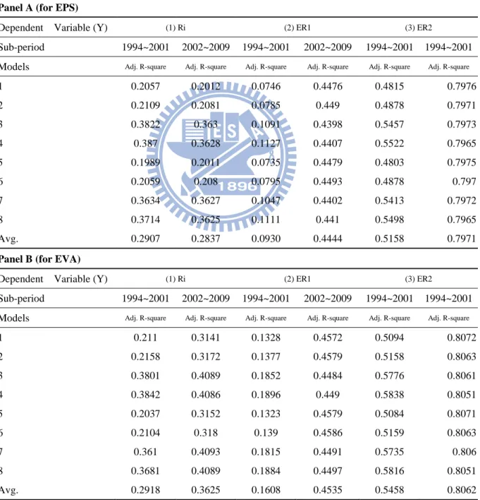
In the sub-period model, we apply identical panel regression models in two sub-periods: 1994–2001 and 2002–2009. Table 5 reports the panel regression results of sub-period model. Empirical results based on Table 5 show that the explanatory power of the former sub-period is lower than the latter sub-period; thus, it fails to confirm H2. The explanatory power of the market risk factors of Fama and French reduces over time due to the rising perspective of behavior finance.
Table 5 Panel Regression -Sub-period Model
This table reports the adj-R2 of regression but omits the associated F-statistics from the panel regression model with fixed effect and no intercept settings for two sub-periods, 1994 to 2001 and 2002 to 2009. The regression coefficients here are omitted in the final table. The number of total sample of firm years (N) is 880 for every model in each sub-period. Three dependent variables including stock returns, excess stock returns 1, and excess stock returns 2 are all used in each model, and two earning-based valuation indicators, EPS and EVA are used as major independent variables. In Panel A, EPS is used as earning-based valuation indicator, while in Panel B, EVA is used instead. Each panel summarizes all model combinations composed of controlled variables: size, tangibility 1, tangibility 2, profitability, investment, Tobin’s Q, current ratio, times interest earned, and debt ratio. (The detailed definition is listed in Table 1.) For example, Model 1 in Panel A indicates three regression results, which are conducted by three dependent variables explained by EPS as the major independent variable plus first combinations of controlled variables in the model.
*, **, and *** indicate significance at 10%, 5%, and 1%, respectively.
Panel A (for EPS)
Dependent Variable (Y) (1) Ri (2) ER1 (3) ER2
Sub-period 1994~2001 2002~2009 1994~2001 2002~2009 1994~2001 1994~2001 Models Adj. R-square Adj. R-square Adj. R-square Adj. R-square Adj. R-square Adj. R-square
1 0.2057 0.2012 0.0746 0.4048 0.4815 0.7976 2 0.2109 0.2081 0.0785 0.3603 0.4878 0.7971 3 0.3822 0.363 0.1091 0.3677 0.5457 0.7973 4 0.387 0.3628 0.1127 0.375 0.5522 0.7965 5 0.1989 0.2011 0.0735 0.3988 0.4803 0.7975 6 0.2059 0.208 0.0795 0.3398 0.4878 0.797 7 0.3634 0.3627 0.1047 0.3552 0.5413 0.7972 8 0.3714 0.3625 0.1111 0.3623 0.5498 0.7965 Avg. 0.2907 0.2837 0.0930 0.3705 0.5158 0.7971
Panel B (for EVA)
Dependent Variable (Y) (1) Ri (2) ER1 (3) ER2
Sub-period 1994~2001 2002~2009 1994~2001 2002~2009 1994~2001 1994~2001 Models Adj. R-square Adj. R-square Adj. R-square Adj. R-square Adj. R-square Adj. R-square
1 0.211 0.3141 0.1328 0.4194 0.5094 0.8072 2 0.2158 0.3172 0.1377 0.3826 0.5158 0.8063 3 0.3801 0.4089 0.1852 0.3894 0.5776 0.8061 4 0.3842 0.4086 0.1896 0.3919 0.5838 0.8051 5 0.2037 0.3152 0.1323 0.4082 0.5084 0.8071 6 0.2104 0.318 0.139 0.3603 0.5159 0.8063 7 0.361 0.4093 0.1815 0.3746 0.5735 0.806 8 0.3681 0.4089 0.1884 0.3781 0.5816 0.8051 Avg. 0.2918 0.3625 0.1608 0.3881 0.5458 0.8062
The result supports EMH instead of behavioral finance, and indicates that our empirical results on behavioral finance effect may not be sufficiently strong to support the
existence of a changing viewpoint from the perspective of behavioral finance. In particular, from Panel A (for EPS) y = Ri case, we can see that the explanatory power of EPS to stock returns appears to slightly decrease over time (Avg: 0.2907 > 0.2837). This suggests the use of EVA as well.
3.3. Causality Model
Table 6 reports the two-way Granger Causality and Wald test results. The first column with H0:X do not affect Y is to test EMH, and the second column of H0:Y do not affect X
is to test behavioral finance effect. Empirical results based on causality tests in Table 6 show that reverse causalities are detectable in all three steps of causality, which confirms H3 (Figures in column 2 are more significant than figures in column 1). There exists a reverse causality relationship (behavioral finance effect) between stock returns (valuation from market perspective), earnings (valuation from operating perspective), and financial constraints (FC).
In the first step of causality (I) [i.e., causality between financial constraints (FC) and operating perspective (OP)], asset size affects EPS and EVA, and vice versa; however, EVA affects tangibility 1 and 2. We document that for asset size, two-way causality (feedback) exists between financial constraints and operating perspective; however, for tangibility 1 and 2, only reverse causality exists. This may correspond to some empirical findings that it is superior to the univariate series in predicting future investments, but not in predicting future earnings (Bar-Yosef, Callen, & Livnat, 1987), and sometimes suggests the existence of earning management problem.
In the second step of causality (II) [i.e., causality between operating perspective and market perspective], EPS and EVA affect stock returns and excess returns 2, and vice versa. We document that two-way causality fully exists between operating perspective and market perspective. As a possible explanation, a previous study states that individual investors may lose money around earnings announcements, experience poor post-trade returns, exhibit the
disposition effect, and make contrarian trades because of reverse causality from behavioral biases to order choices (Linnainmaa, 2010).
In the third step of causality (III) [i.e., causality between financial constraints and market perspective] asset size and tangibility 1 affect stock returns and excess returns 2, and vice versa. However, tangibility 2 affects excess returns 2, and stock returns affect
tangibility 2. We document that to asset size and tangibility 1, two-way causality fully exists between financial constraints and market perspective; however, with tangibility 2 to stock returns, only reverse causality exists. If we interpret the causality here as leadership, informed traders who influence stock price may be one source of behavioral finance effect (Peiers, 1997).
We also state that EVA and ER2 have a tendency of stronger causality. In (I) and (II) of Table 6, we find that the number of χ2-statistics of EVA are all bigger than those of EPS, except for EPS, which affects Ri (21.79 < 94.37). In (II) and (III), χ2-statistics of ER2 are all bigger than those of Ri.
Table 6 Two-way Granger Causality and Wald Test
This table reports the three-step results of two-way Granger Causality and Wald tests with the associated
χ2-statistics and null hypothesis for whole sample period from 1994 to 2009. Information statistics and optimal lag
numbers of time series models here are omitted in the final table. The number of total sample of firm years (N) is 1760. The two-way Granger Causality and Wald tests are built to tests two null hypothesis at one time: H0, the independent variable (X) does not cause the dependent variable (Y); and H0, The dependent variable (Y) does not cause the independent variable (X)]. Thus, we sequentially set three-step causality tests as follows:
(I) Three measures of financial constraints (FC) as (X), and two measures of valuations from operating perspective (OP) as (Y); to investigate the causality between FC and OP.
(II) Two measures of valuations from operating perspective (OP) as (X), and two measures of valuations from market perspective (MP) as (Y); to investigate the causality between OP and MP.
(III) Three measures of financial constraints (FC) as (X), and two measures of valuations from market perspective (MP) as (Y); to investigate the causality between FC and MP.
Three possible outcomes in causality model are used to describe causality: independency (i.e., Do not reject both two-way H0 at the same time), unidirectionality (i.e., Reject 1-way H0; and we refer rejecting H0: (Y) does not cause (X) as “reverse causality”), and feedback (i.e., Reject both 2-ways H0.)
Three measures of financial constraints (FC) include asset size (ln(TA)), asset tangibility 1(Tang1), and asset tangibility 2 (Tang2); two measures of valuations from operating perspective (OP) include EPS and EVA; two measures of valuations from market perspective (MP) include stock returns (Ri) and excess stock returns 2(ER2). *, **, and *** indicate significance at 10%, 5%, and 1% respectively.
(I) Causality between Financial constraints (FC) and Operating Perspective (OP)
Granger-Causality Wald Test
H0:Financing Constraints(X) do not cause Valuation(Y)
H0:Valuation(Y) do not cause Financing Constraints(X) Dependent Variable (Y) (1) EPS (2) EVA (1) EPS (2) EVA
Variable(X) χ2 χ2 χ2 χ2 Financial constraints (FC) as (X) ln(TA) 13.57 * 45.05 *** 47.88 *** 231.13 *** ← → Tang1 3.86 5.59 4.6 34.36 *** Operating Perspective (OP) as (Y) Tang2 9.02 8.02 6.28 25.18 ***
(II) Causality between Operating Perspective (OP) and Market Perspective (MP)
Granger-Causality Wald Test
H0:Valuation(X) do not cause Market Stock Returns(Y)
H0:Market Stock Returns(Y) do not cause Valuation(X) Dependent Variable (Y) (1) Ri (2) ER2 (1) Ri (2) ER2
Variable(X) χ2 χ2 χ2 χ2 Operating Perspective (OP) as (X) ← → EPS 94.37 *** 96.74 *** 53.7 *** 72.86 *** Market Perspective (MP) as (Y) EVA 21.79 *** 920.02 *** 86.83 *** 133.25 ***
(III) Causality between Financial Constraints (FC) and Market Perspective (MP)
Granger-Causality Wald Test
H0:Financing Constraints(X) do not cause Valuation(Y)
H0:Valuation(Y) do not cause Financing Constraints (X) Dependent Variable (Y) (1) Ri (2) ER2 (1) Ri (2) ER2
Variable(X) χ2 χ2 χ2 χ2 Financial constraints (FC) as (X) ln(TA) 85.32 *** 218.13 *** 112.31 *** 306.54 *** ← → Tang1 32.66 *** 65.88 *** 18.55 *** 76.55 *** Market Perspective (MP) as (Y) Tang2 11.88 44.61 *** 44.18 *** 110.06 ***
3.4. Robustness Check
In this section, we provide the panel regression results of whole sample and sub-period models. However, we adjust clustered robust standard errors, as proposed by Petersen (2009), to serve as robustness check in order to avoid possible spurious relationship on panel regressions and to increase credibility on regression coefficients.
Table 7 Panel Regression – Sub-period Model Adjusted by Clustered Robust Standard Errors
This table reports the adj-R2 of regression, but omits the associated F-statistics (in parentheses) from the panel regression model with fixed effect and no intercept settings for two sub-periods, 1994 to 2001 and 2002 to 2009, adjusted by clustered robust standard errors, as proposed by Petersen (2009). Regression coefficients here are omitted in final table. The number of total sample firm years (N) is 880 for every model in each sub-period. Three dependent variables, including stock returns, excess stock returns 1, and excess stock returns 2 are all used in each model, and two earning-based valuation indicators, EPS and EVA are used as major independent variables. In Panel A, EPS is used as earning-based valuation indicator, whereas in Panel B, EVA is used instead. Each panel summarizes all model combinations composed of controlled variables: size, tangibility 1, tangibility 2, profitability, investment, Tobin’s Q, current ratio, times interest earned, and debt ratio (the detailed definition is listed in Table 1.) For example, Model 1 in Panel A, indicates three regression results, which are conducted by three dependent variables explained by EPS as major independent variable plus the first combinations of controlled variables in model.
*, **, and *** indicate significance at 10%, 5%, and 1%, respectively.
Panel A (for EPS)
Dependent Variable (Y) (1) Ri (2) ER1 (3) ER2
Sub-period 1994~2001 2002~2009 1994~2001 2002~2009 1994~2001 1994~2001 Models Adj. R-square Adj. R-square Adj. R-square Adj. R-square Adj. R-square Adj. R-square
1 0.2057 0.2012 0.0746 0.4476 0.4815 0.7976 2 0.2109 0.2081 0.0785 0.449 0.4878 0.7971 3 0.3822 0.363 0.1091 0.4398 0.5457 0.7973 4 0.387 0.3628 0.1127 0.4407 0.5522 0.7965 5 0.1989 0.2011 0.0735 0.4479 0.4803 0.7975 6 0.2059 0.208 0.0795 0.4493 0.4878 0.797 7 0.3634 0.3627 0.1047 0.4402 0.5413 0.7972 8 0.3714 0.3625 0.1111 0.441 0.5498 0.7965 Avg. 0.2907 0.2837 0.0930 0.4444 0.5158 0.7971
Panel B (for EVA)
Dependent Variable (Y) (1) Ri (2) ER1 (3) ER2
Sub-period 1994~2001 2002~2009 1994~2001 2002~2009 1994~2001 1994~2001 Models Adj. R-square Adj. R-square Adj. R-square Adj. R-square Adj. R-square Adj. R-square
1 0.211 0.3141 0.1328 0.4572 0.5094 0.8072 2 0.2158 0.3172 0.1377 0.4579 0.5158 0.8063 3 0.3801 0.4089 0.1852 0.4484 0.5776 0.8061 4 0.3842 0.4086 0.1896 0.449 0.5838 0.8051 5 0.2037 0.3152 0.1323 0.4579 0.5084 0.8071 6 0.2104 0.318 0.139 0.4586 0.5159 0.8063 7 0.361 0.4093 0.1815 0.4491 0.5735 0.806 8 0.3681 0.4089 0.1884 0.4497 0.5816 0.8051 Avg. 0.2918 0.3625 0.1608 0.4535 0.5458 0.8062
Tables of the panel regression results of whole sample model for EPS and EVA, adjusted by clustered robust standard errors, are the same as Table 3 and Table 4 after rounding to the 3rd decimal place. Table 7 reports the panel regression results of the sub-period model adjusted by clustered robust standard errors.
After adjustments, we find smaller estimating errors on panel regression coefficient estimates, which are decreasing and accurate to the 2nd–3rd decimal place in both models. Empirical results remain close to the original before adjustments in whole sample model, and it only differs in the explanatory power of dependent variables taking ER1 in the sub-period model in Table 7 (0.4444 > 0.3705;0.4535 > 0.3881), which may due to improvement or missing value.
Besides, we also take addition VIF test to illustrate the collinearity problem is not severe here (VIF < 10, tolerance > 0.1). Furthermore, we consider the endogenous problem by providing another panel regression result of changing X into Y & Y into X in Table 8, and we still get the same result that the coefficients of EPS and EVA to stock returns (Ri) appear in counter signs. EPS is mostly positively related to Ri, while EVA is negatively related to Ri. The significance and signs on coefficients of control variables only slightly differ, so it is consistent with our previous findings.
Table 8 Panel Regression — Whole Sample Model for Returns to Earnings
This table reports the regression coefficients but omits the associated F-statistics and t-statistics from the panel regression model with fixed effect and no intercept settings for whole sample period 1994 to 2009. The number of total sample firm-years (N) is 1760 for every model. Three major independent variables are all used in each model, including stock returns, excess stock returns 1, and excess stock returns 2, and two earning-based valuation indicators EPS and EVA are used as the dependent variables. The table summarizes all model combinations composed of controlled variables: size, tangibility 1, tangibility 2, profitability, investment, Tobin’s Q, current ratio times interest earned, and debt ratio. (The detailed definition is listed in Table 1.) For example, Model 1 in Panel A indicates three regression results conducted by y=EPS and each three returns (Ri,ER1,ER2) as independent variables plus first combinations of controlled variables in the model; in Panel B, y=EVA. *, **, and *** indicate significance at 10%, 5%, and 1%, respectively.