一個有效解決日本益智遊戲「發現小花」的演算法

全文

(1)!. ୮ Ҥ ҫ ೮ δ Ꮱ! !. !. !. !. !. 資訊科學與工程研究所碩士論文. 一個有效解決日本益智遊戲「發現小花」的演算法 An Efficient Algorithm for Solving Japanese Puzzles. 研究生：尤瓊雪指導教授：陳玲慧. 教授. 中華民國九十六年一月.

(2) 一個有效解決日本益智遊戲「發現小花」的演算法 An Efficient Algorithm for Solving Japanese Puzzles. 研究生：尤瓊雪. Student ：Chiung-Hsueh Yu. 指導教授：陳玲慧. Advisor：Ling-Hwei Chen. 國立交通大學資訊科學與工程研究所碩士論文. A Thesis Submitted to Institute of Computer Science and Engineering College of Computer Science National Chiao Tung University in Partial Fulfillment of the Requirements for the Degree of Master in Computer Science January 2007 Hsinchu, Taiwan, Republic of China. 中華民國九十六年一月.

(3) 一個有效解決日本益智遊戲「發現小花」的演算法研究生：尤瓊雪. 指導教授：陳玲慧博士. 國立交通大學資訊科學與工程研究所碩士班. 摘. 要. 日本益智遊戲「發現小花」是風行於日本與荷蘭的邏輯遊戲之一，而「該謎題是否能解」是一個難以回答的問題，甚至是一個非決定性多項式時間-完全（NP-complete）問題。目前已有一些相關論文提出，有的是利用基因演算法解決，但是可能造成錯誤的答案出現；而有的是利用深先搜尋演算法，該演算法是一種暴力搜尋法，所以執行速度很慢；因此，在這篇論文裡，我們想要提出一種演算法來盡可能快速的解決所有謎題，這個演算法不只加速了深先搜尋法的速度，更確保了謎題解答的正確性。在這個遊戲裡，很多謎題是緊密而連續的圖形，我們可因此推導出一些邏輯規則，按照這些規則去填出那些可以馬上決定位置的格子；然而，並非所有謎題都可以依邏輯規則完全解出，像是有些隨意產生的謎題需要另一種方法來輔助，在這種情況下，我們使用深先搜尋演算法，但為了加快執行速度，分支界限法的觀念被引進，其目的是提早終止那些不合法的路徑。實驗的結果顯示，我們的演算法成功地解決日本益智遊戲「發現小花」，而執行速度也比一般的深先搜尋法來得快速。. I.

(4) An Efficient Algorithm for Solving Japanese Puzzles Student: Chiung-Hsueh Yu. Advisor: Dr. Ling-Hwei Chen. Institute of Computer Science and Engineering National Chiao Tung University. ABSTRACT. Japanese puzzle is one of logical games popular in Japan and Netherlands. The question “Is this puzzle solvable?” is difficult to answer, even is an NP-complete problem. At present, there have been some related papers proposed. Some use genetic algorithm (GA), but the solution may be wrong. Some use depth first search (DFS) algorithm. The DFS algorithm is an exhaustive search, so the execution speed is slow. Hence, in this thesis, we want to propose an algorithm to solve puzzles as quickly as possible. The algorithm not only accelerates the speed of DFS but also ensures the correctness of the solution of a puzzle. In this puzzle game, many puzzles are compact and contiguous pictures. Based on this, we can deduce some logical rules, and use these rules to paint those cells whose positions can be determined immediately. However, not all puzzles can be solved completely by logical rules. In this situation, we use the DFS algorithm to complete the puzzle solving. In order to speed up the process, the “branch and bound” technique is used to do early termination for those impossible paths. Experimental results show that our algorithm can solve Japanese puzzles successfully, and the processing speed is significantly faster than that of DFS.. II.

(5) 誌. 謝. 這篇論文的完成，首先要感謝指導教授陳玲慧博士讓我加入自動化資訊處理實驗室的研究群，並且在這兩年多來不斷的細心指導，不管是在學業上或是生活上，老師的提醒、包容與體諒，都帶給了我不少的助益，在此，再次謝謝老師。此外，感謝口試委員蔡月霞教授、陳佑冠教授以及何俊達教授於口試中給予的指導與建議，才能使這篇論文更加完善。接著要謝謝實驗室一起研究的可愛伙伴們：民全、萓聖、惠龍和文超四位學長，以及維中、芳如、佩瑩、立人、俊旻、信嘉、薰瑩、子翔和偉全九位學弟妹；不管是在研究上給我的指導與叮嚀，或是在日常生活上製造的有趣話題，還有經歷過實驗室一些大大小小的事情後，那股仍不曾改變的向心力與凝聚力；如果沒有你們，我想我的研究生活一定會少了很多樂趣與知識的增長。此外，要謝謝我的大學同學和室友們：阿信、建凱、阿福、小美、狼鼠、薇安、綿等等，讓我在沒有實驗室同屆同學的狀況下，能夠有人可以一起作伴，不管是課業上的互相討論，或是生活上的談心笑鬧，謝謝你們聽我說話、幫我打氣，陪我度過一些心理上的波折。最後，當然要謝謝我的家人：媽媽及哥哥們。謝謝你們對我沒能如期畢業的寬容，還盡可能的提供我經濟上的支出，更謝謝媽媽長期當我的傾聽者；另外，也謝謝每天都來迎接我回家的噹噹。能和你們成為一家人，是我這輩子感到最幸運且最幸福的事，謹以此篇論文獻給你們，也獻給所有我關心以及關心我的人。 III.

(6) CONTENTS ABSTRACT (IN CHINESE) ......................................................................................... I ABSTRACT.................................................................................................................. II ACKNOWLEDGE (IN CHINESE).............................................................................III CONTENTS.................................................................................................................IV LIST OF FIGURES ......................................................................................................V LIST OF TABLES ..................................................................................................... VII CHAPTER 1 INTRODUCTION ................................................................................1 1.1 Motivation........................................................................................................1 1.2 Japanese Puzzles ..............................................................................................1 1.3 Previous Works ................................................................................................2 1.4 Organization of the Thesis ...............................................................................5 CHAPTER 2 PROPOSED METHOD........................................................................6 2.1 The first phase: Logical rules (LR) ..................................................................7 2.2 The second phase: DFS with branch and bound ............................................22 CHAPTER 3 EXPERIMENTAL RESULTS ............................................................26 CHAPTER 4 CONCLUSIONS ................................................................................31 CHAPTER 5 FUTURE WORKS .............................................................................32 REFERENCES ............................................................................................................33. IV.

(7) LIST OF FIGURES Fig. 1.1 Japanese puzzle. (a) A simple puzzle. (b) The solution of (a)..........................2 Fig. 1.2 A puzzle with two solutions..............................................................................2 Fig. 1.3 A puzzle with no solution. ................................................................................2 Fig. 1.4 DT problem and Japanese puzzle. (a) DT problem. (b) Japanese puzzle.........3 Fig. 1.5 A puzzle problem..............................................................................................4 Fig. 1.6 The DFS tree of Fig. 1.5...................................................................................4 Fig. 1.7 Six possible solutions in the DFS tree..............................................................4 Fig. 1.8 Verification process for the different cases. .....................................................5 Fig. 2.1 The flowchart of the proposed method.............................................................6 Fig. 2.2 An illustration of range. (a) A special row of a puzzle. (b) The left-most case of (a). (c) The right-most case of (a)................................................................9 Fig. 2.3 An example of Rule 1.1..................................................................................10 Fig. 2.4 An example of Rule 1.2. (a) One row of a puzzle with a partial painting result. (b) The result of applying Rule 1.2 to (a). ..........................................10 Fig. 2.5 An example of Rule 1.3. (a) One row of a puzzle with a partial painting result. (b) The cell cr js belongs to the third black run with length one. (c) The cell cr js is the head cell of the last black run............................................ 11 Fig. 2.6 An example of Rule 1.4. (a) One row of a puzzle with a partial painting result ( maxL =3). (b) The new black segment’s length after coloring ci is 4. (c) The cell ci should be left empty. .................................................................12 Fig. 2.7 An example of Rule 1.5. (a) Top: one row of a puzzle with a partial painting result. Middle: all possible solutions for ci . Bottom: the result of applying Rule 1.5 to top figure. (b) Top: a special case (all black runs containing ci have the same length). Bottom: the result of applying Rule 1.5 to top figure. ........................................................................................................................14 Fig. 2.8 An example of Rule 2.3..................................................................................16 Fig. 2.9 An example of Rule 3.1. (a) One row of a puzzle with a partial painting result. (b) The result of applying Rule 3.1 to (a). ..........................................16 Fig. 2.10 An example of Rule 3.2. (a) One row of a puzzle with a partial painting result. (b) The result of applying Rule 3.2 to (a). ........................................17 Fig. 2.11 An example of Rule 3.3-1. (a) One row of a puzzle with a partial painting result. (b) The result of applying Rule 3.3-1 to (a). .....................................19 Fig. 2.12 An example of Rule 3.3-2. (a) One row of a puzzle with a partial painting result. (b) The result of applying Rule 3.3-2 to (a). .....................................19. V.

(8) Fig. 2.13 An example of Rule 3.3-3. (a) One row of a puzzle with a partial painting result. (b) The length of coloring those cells between cs and ce is 5. (c) The result of applying Rule 3.3-3 to (a).......................................................20 Fig. 2.14 An example of DFS. (a) A given puzzle. (b) The possible solutions of row 1. (c) The possible solutions of row 2. (d) A rough tree of (a).........................23 Fig. 2.15 The process of DFS with branch and bound. (a) The deduced result of row 2 based on the first possible solution of row 1. (b) The deduced result of row 2 based on the second possible solution of row 1. (c) The deduced result of row 2 based on the third possible solution of row 1. (d) The first possible solution of row 2 corresponding to (c). (e) The final solution.....................24 Fig. 2.16 An example before using DFS. (a) The original puzzle. (b) The resulting puzzle executed by LR.................................................................................25 Fig. 3.1 Test images. (a) Sheep (25x25). (b) Airplane (25x25). (c) Random_1 (30x30). (d) Monkey (15x15). (e) Sunflower (25x25). (f) Random_2 (30x30)...........27 Fig. 3.2 An illustration of scattering. (a) 10 possible solutions. (b) 21 possible solutions. (c) 36 possible solutions. (d) 56 possible solutions.......................27 Fig. 3.3 An illustration of chain relation. More “○” means the puzzle is more connected. (a) The magnified picture of part of Fig. 3.1 (c). (b) The magnified picture of part of Fig. 3.1 (f). ........................................................28 Fig. 3.4 A 7x8 puzzle with many solutions. (a) The result after LR. (b) The first solution. (c) The second solution. ..................................................................28 Fig. 3.5 A puzzle with no solution. ..............................................................................29 Fig. 3.6 GA gives a wrong answer of Fig. 3.5. ............................................................29 Fig. 3.7 Test images. (a) Flower_word (10x10). (b) Hippo (20x20). (c) Formosa (25x25). (d) Snoopy (25x25). (e) Owl (30x25). (f) Skating (30x25). ...........29 Fig. 5.1 Generator. (a) The input image. (b) The puzzle generated. (c) The result of the puzzle. ............................................................................................................32. VI.

(9) LIST OF TABLES Table 1 The comparison of the experimental results between surveyed paper and our Table 1 algorithm.........................................................................................................30. VII.

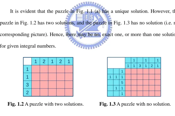
(10) CHAPTER 1 INTRODUCTION 1.1 Motivation Japanese puzzle, also known as nonogram, is one of logical games popular in Japan and Netherlands. The game is recommended to Taiwan recently, but few papers are concerned with this topic – Japanese nonograms. In addition, some related papers solved this problem by non-logical algorithms, and the execution speed is slow. On the other hand, the question “Is this puzzle solvable?” turns out to be very hard to answer in general, even is a NP-complete problem [1-2]. In this thesis, we will present a fast method to solve this problem. First, we will provide some logical rules to solve most part of a puzzle, and then use DFS with branch and bound scheme to solve the remaining part. The detail of our proposed method will be described in Chapter 2.. 1.2 Japanese Puzzles Japanese puzzles will be described in this section. Fig. 1.1 (a) is a simple puzzle and Fig. 1.1 (b) is the solution of Fig. 1.1 (a). Ignoring the numbers, the solution can be considered as a black-white (1-and-0) picture. Here, we use ■ as a colored (black) cell, □ as an empty (white) cell, and ■ as an unknown cell (i.e. an undetermined cell). The positive integers alongside the rows and columns give the information about the lengths of black runs (a black run: contiguous black cells) in that row or column respectively. The goal is to paint the cells to form a picture that satisfies the following constraints:. 1.

(11) 1. Each cell must be colored (black) or left empty (white). 2. If a row or column has k numbers: s1 , s 2 , …, sk , then it must contain k black runs – the first (leftmost for rows / topmost for columns) black run with the length s1 , the second black run with the length s 2 , and so on. 3. There should be at least one empty cell between two consecutive black runs.. (a). (b). Fig. 1.1 Japanese puzzle. (a) A simple puzzle. (b) The solution of (a).. It is evident that the puzzle in Fig. 1.1 (a) has a unique solution. However, the puzzle in Fig. 1.2 has two solutions, and the puzzle in Fig. 1.3 has no solution (i.e. no corresponding picture). Hence, there may be no, exact one, or more than one solution for given integral numbers. 1. 2. 1. 2. 1. 1 1. 1. 1. 1 3. 1. 1 2. 1. 1. 1. 1. 1. 1 5. 3. 1. 2. 1 1. Fig. 1.2 A puzzle with two solutions.. Fig. 1.3 A puzzle with no solution.. 1.3 Previous Works In 2004, Batenburg [3] described an evolutionary algorithm for discrete tomography (DT). And then Batenburg Kosters [4] provided a method to solve Japanese puzzle. By modifying the fitness function in [3], the evolutionary algorithm 2.

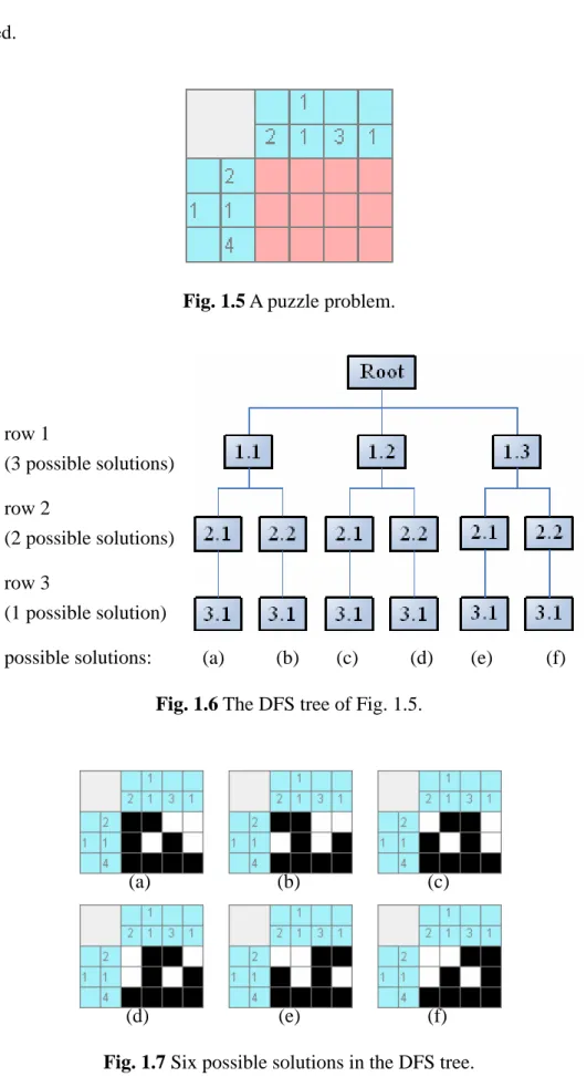
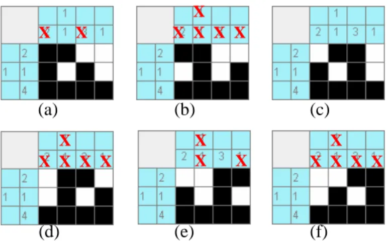
(12) can be used to solve Japanese puzzle. DT is concerned with the reconstruction of a discrete image from its projections [4]. Japanese puzzles can be considered as a special form of the DT problem. Fig. 1.4 shows an example to explain the difference between them. Since the evolutionary algorithm in [3] will converge to a local optimum, the obtained solution may be incorrect.. (a) (b) Fig. 1.4 DT problem and Japanese puzzle. (a) DT problem. (b) Japanese puzzle.. In 2004, Wiggers [4] proposed a genetic algorithm (GA) and a depth first search (DFS) algorithm to solve Japanese puzzles. He also compared the performance of these two algorithms. For a puzzle of small size, DFS algorithm is faster than GA; otherwise, GA is faster. However, both methods are slow. In the following, we will give a brief description for the DFS algorithm, since it will also be used in our proposed method.. [Depth First Search (DFS)] It is a straightforward idea to solve the Japanese nonogram by DFS. The author generates all possible solutions of each row. Taking Fig. 1.5 as an example, Fig. 1.6 is its corresponding DFS tree and Fig. 1.7 shows all possible solutions in the tree. Each possible solution corresponds to a path from root to a leaf node, find all paths using DFS and then use the column information of the puzzle to verify each possible solution. A possible solution will be considered as a true solution, if it satisfies all 3.

(13) columns’ restrictions. Fig. 1.8 (c) is the only correct solution after the verification process. Note that the symbol “X” in Fig. 1.8 stands for the column’s restriction not satisfied.. Fig. 1.5 A puzzle problem.. row 1 (3 possible solutions) row 2 (2 possible solutions) row 3 (1 possible solution) possible solutions:. (a). (b). (c). (d). (e). Fig. 1.6 The DFS tree of Fig. 1.5.. (a). (b). (c). (d). (e). (f). Fig. 1.7 Six possible solutions in the DFS tree. 4. (f).

(14) X. X. (a). X X X X X. (b) X X. X X X X X. (d). (e). (c) X. X X X X X. (f). Fig. 1.8 Verification process for the different cases.. Whether the evolutionary algorithm presented in [4] or the genetic algorithm (GA) described in [5], both of them will converge to a local optimum, so sometimes the obtained solution may not be correct. Besides, the depth first search (DFS) algorithm proposed in [5] takes longer time than GA when solving large puzzles. However, DFS will always find correct solutions. In this thesis, some logical rules (LR) are provided to determine the unknown cells in a Japanese puzzle as many as possible, and then DFS is used to solve those remaining unknown cells. In order to speed up the process, the “branch and bound” technique is used to do early termination for those impossible paths.. 1.4 Organization of the Thesis This thesis is composed of five chapters. In Chapter 1, Japanese puzzles and previous works are introduced. And then, the remainder of this thesis is organized as follows. Our proposed algorithm for solving Japanese puzzles will be presented in Chapter 2. In Chapter 3, several experimental results will be shown. Finally, conclusions and future works will be given in the last two chapters.. 5.

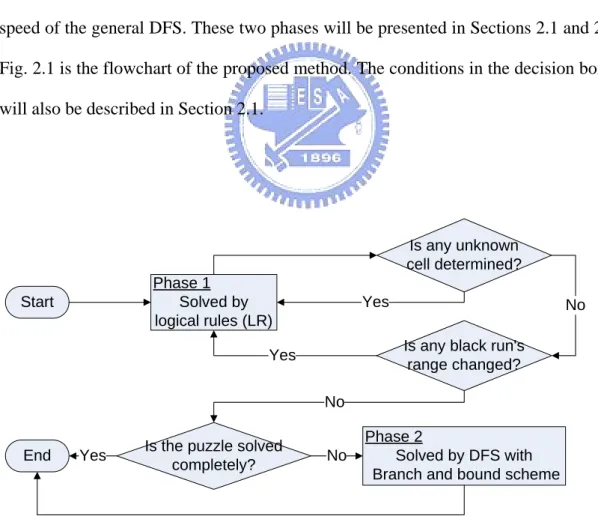
(15) CHAPTER 2 PROPOSED METHOD In general Japanese puzzle game, we usually paint those cells which can be determined immediately at first. Then, the rest of undetermined cells will be solved by guess. Based on this fact, we will propose a method to solve Japanese puzzles automatically. The method contains two phases. In the first phase, some logical rules are deduced and used to determine some cells; in the second phase, another method, the depth first search will be applied to solve those remaining unknown cells. Furthermore, the “branch and bound” technique is used to accelerate the searching speed of the general DFS. These two phases will be presented in Sections 2.1 and 2.2. Fig. 2.1 is the flowchart of the proposed method. The conditions in the decision boxes will also be described in Section 2.1.. Is any unknown cell determined? Phase 1 Solved by logical rules (LR). Start. Yes. No Is any black run's range changed?. Yes No End. Yes. Is the puzzle solved completely?. No. Phase 2 Solved by DFS with Branch and bound scheme. Fig. 2.1 The flowchart of the proposed method.. 6.

(16) 2.1 The first phase: Logical rules (LR) One may also use some skills to solve Japanese puzzles, like the rules described in [6]. In this phase, eleven rules are proposed but we present a new concept of range of a black run (“range” will be explained later). These rules can be divided into three main parts. The first part is to determine which cells should be colored or left empty, the second part is to refine the ranges of black runs, and the third is not only to determine which cells should be colored or left empty but also to refine the ranges of black runs. The first five rules belong to part I, the following three rules belong to part II, and the last three rules belong to part III. Each rule will be applied in each row and then in each column. The total eleven rules are executed sequentially and iteratively. In the beginning, all cells in the puzzle are considered as unknown. In some iterations, some unknown cells will be determined as colored cells or empty ones. However, in some iterations, maybe only the ranges of some possible black runs are refined. That is, there are not always some unknown cells determined in each iteration. Thus, if no unknown cell is determined and no black run’s range is changed, we will stop using logical rules because there will be no changes in later iterations. Note that, the rules applied in a row are the same as those applied in a column, so we only take a row as an example to explain our algorithm.. Preliminary The position where a black run may be placed plays an important role. An idea about the range (rjs , rje ) of a black run j is proposed, where r js stands for the. left-most starting position of the run, and r je stands for the right-most ending position of the run. That is, black run j can only be placed between r js and r je . If the range of each black run is precisely estimated, these ranges information can help. 7.

(17) us to solve puzzles quickly. In the beginning, the initial range of a black run in a row is set between the left-most possible position and the right-most possible position. For each black run, it must reserve some cells for the former black runs and the later ones. Fig. 2.2 shows an example. Fig. 2.2 (a) shows a special row of a puzzle, in this row, there are three black runs with lengths 1, 3, and 2, respectively. Fig. 2.2 (b) shows the left-most possible solution of Fig. 2.2 (a) for each run, the first cell is colored and there is only one empty cell between every two neighboring black runs. Fig. 2.2 (c) shows the right-most possible solution of Fig. 2.2 (a) for each run, the last cell is colored and there is only one empty cell between every two neighboring black runs. Now, we take the second run as an example to do more detail explanation. In Fig. 2.2 (b), the left-most position, at which the first cell of the second black run can start, is the third position. The reason is that there must reserve at least two cells in the head, one cell is reserved for the first black run and the other is reserved for the empty cell between the first and second black runs. Similarly, the right-most position, at which the last cell of the second black run can appear, is the seventh position. That is due to that there must reserve at least three cells in the tail, two cells are reserved for the third black run and one cell is reserved for the empty cell between the second and third black runs.. Initial run range estimating. We let the size of each row with k black runs be n and the cells in a row with index (0, K, n-1) , we can use the following formula to determine the initial range of. each black run. Specially, r js of the first black run is initialized 0 and r je of the last black run is initialized (n-1) .. 8.

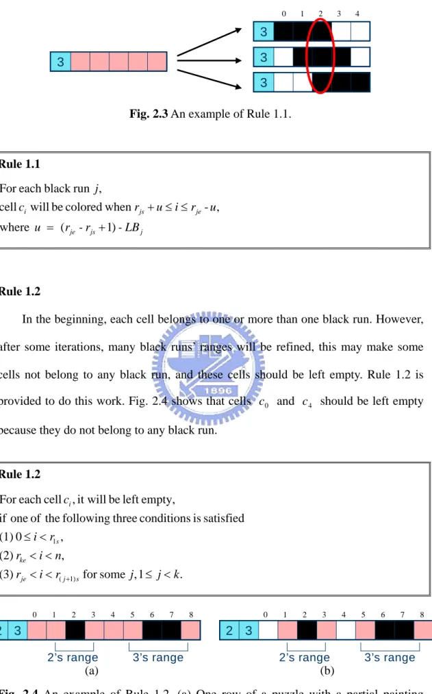
(18) j-1. r js = ∑ ( LBi + 1), i =1. r je = (n-1) -. ∀ j = 1, K, k .. k. ∑ ( LB + 1), i. i = j +1. where LBi is the length of black run i . Using the above formula, we can get the initial ranges of the three black runs in Fig. 2.2 (a), which are (0, 2), (2, 6), and (6, 9), respectively. 0. (a). 1 3 2. (b). 1 3 2. (c). 1 3 2. 1. 2. 3. 4. 5. 6. 7. 8. 9. Fig. 2.2 An illustration of range. (a) A special row of a puzzle. (b) The left-most case. of (a). (c) The right-most case of (a).. Part I There are five rules in this part, all of them are used to determine which cells should be colored (black) or left empty (white). Rule 1.1. For each black run, some cells must be colored if all the possible solutions of the black run have the intersection. Actually, the intersection of all possible solutions is also the intersection of the left-most case of the black run and the right-most case of the black run. It is obvious that the intersection exists when the length of the black run’s range is less than two times the actual length of a black run. Fig. 2.3 is an example. Consequently, we provide Rule 1.1 to paint the cells sure to be colored. In the rule, ci is the cell with index i .. 9.

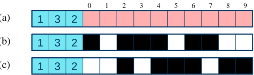
(19) 0. 1. 2. 3. 4. 3 3. 3. 3 Fig. 2.3 An example of Rule 1.1.. Rule 1.1 For each black run j , cell ci will be colored when r js + u ≤ i ≤ r je - u , where u = (rje - rjs + 1) - LB j. Rule 1.2. In the beginning, each cell belongs to one or more than one black run. However, after some iterations, many black runs’ ranges will be refined, this may make some cells not belong to any black run, and these cells should be left empty. Rule 1.2 is provided to do this work. Fig. 2.4 shows that cells c 0 and c 4 should be left empty because they do not belong to any black run.. Rule 1.2 For each cell ci , it will be left empty, if one of the following three conditions is satisfied (1) 0 ≤ i < r1s , (2) rke < i < n, (3) rje < i < r( j +1) s for some j , 1 ≤ j < k . 0. 1. 2. 3. 4. 5. 6. 7. 0. 8. 1. 2. 3. 4. 5. 6. 7. 8. 2 3. 2 3 2’s range. 3’s range. 2’s range. (a). 3’s range. (b). Fig. 2.4 An example of Rule 1.2. (a) One row of a puzzle with a partial painting. result. (b) The result of applying Rule 1.2 to (a). 10.

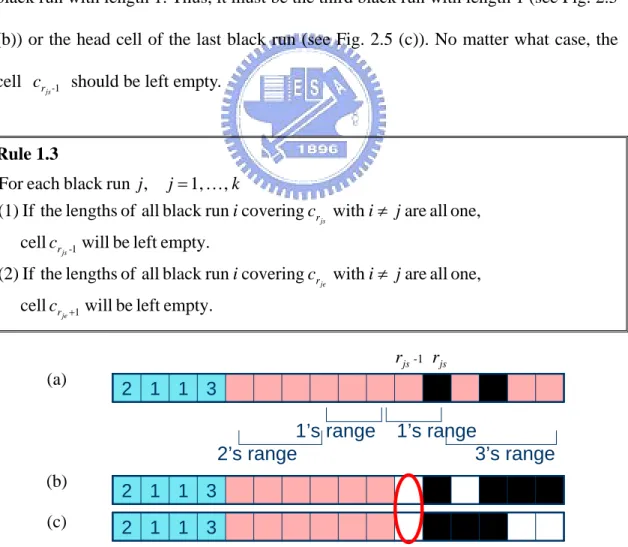
(20) Rule 1.3. For each black run j , when the first cell cr js of its range is colored, we will check cr js covered by what other black runs. If the lengths of those covering black runs are all one, the cell cr js -1 should be left empty. In the similar way, when the last cell cr je of its range is colored, we will check cr je covered by what other black runs. If the lengths of those covering black runs are all one, the cell cr je +1 should be left empty. We provide Rule 1.3 to determine whether cells cr js -1 and cr je +1 should be left empty. Taking Fig. 2.5 as an example, the colored cell cr js in Fig. 2.5 (a) is the first cell of the range of the last black run with length 3. It is also covered by the third black run with length 1. Thus, it must be the third black run with length 1 (see Fig. 2.5 (b)) or the head cell of the last black run (see Fig. 2.5 (c)). No matter what case, the cell cr js -1 should be left empty.. Rule 1.3. For each black run j , j = 1, K, k (1) If the lengths of all black run i covering cr js with i ≠ j are all one, cell cr js -1 will be left empty. (2) If the lengths of all black run i covering cr je with i ≠ j are all one, cell cr je +1 will be left empty. rjs -1 rjs (a). 2 1 1 3. 1’s range 2’s range (b) (c). 1’s range 3’s range. 2 1 1 3 2 1 1 3. Fig. 2.5 An example of Rule 1.3. (a) One row of a puzzle with a partial painting result. (b) The cell cr js belongs to the third black run with length one. (c) The cell cr js is the head cell of the last black run. 11.

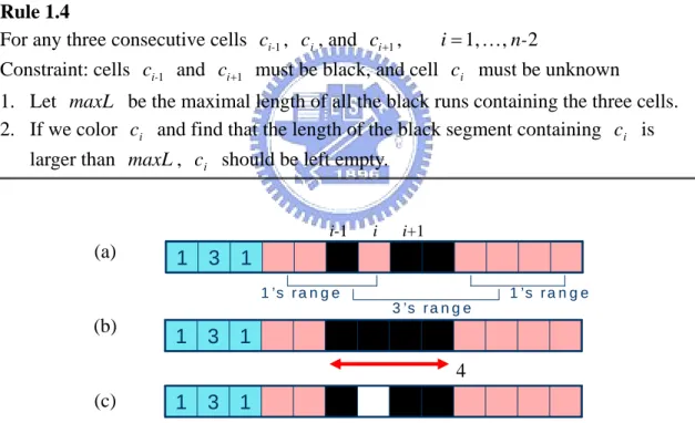
(21) Rule 1.4. There may be some short black segments existing in a row. If any two consecutive black segments with an unknown cell between them are combined into a new black segment with length larger than the maximal length of all black runs containing part of this new segment, the unknown cell should be left empty. Rule 1.4 is provided to deal with this situation. Fig. 2.6 shows an example. From Fig. 2.6 (b), we can see that by coloring ci , the length of the new black segment is 4. Since the new black segment is covered by two runs with length 1 and 3 and 4 is larger than 3, so we set the unknown cell ci as empty.. Rule 1.4 For any three consecutive cells ci-1 , ci , and ci +1 , i = 1, K, n-2 Constraint: cells ci-1 and ci +1 must be black, and cell ci must be unknown. 1. Let maxL be the maximal length of all the black runs containing the three cells. 2. If we color ci and find that the length of the black segment containing ci is larger than maxL , ci should be left empty.. i-1. (a). i. i+1. 1 3 1 1 ’s r a n g e. 1 ’s r a n g e 3 ’s r a n g e. (b). 1 3 1 4. (c). 1 3 1. Fig. 2.6 An example of Rule 1.4. (a) One row of a puzzle with a partial painting result. ( maxL =3). (b) The new black segment’s length after coloring ci is 4. (c) The cell ci should be left empty.. 12.

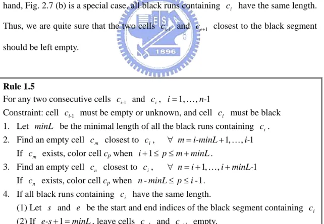
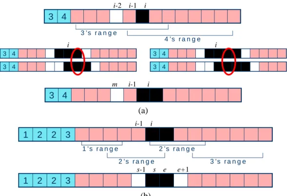
(22) Rule 1.5. Some empty cells like walls may obstruct some black segments expand, we want to color more cells based on this property. For a black segment belonging to series of black runs, which have the same length but the ranges of them overlap each other, if the length of the black segment equals to the length of those black runs covering the black segment, we can set the two cells closest to the black segment as empty. Rule 1.5 is proposed to solve the above problems. Fig. 2.7 is a detailed description. In Fig. 2.7(a), we do not know ci belonging to which black run. However, an empty cell ci -2 obstructs the black segment containing ci to expand to the left side of ci -2 . Hence, no matter ci belongs to the run with length 3 or the run with length 4, the cell next to ci should be colored. On the other hand, Fig. 2.7 (b) is a special case, all black runs containing ci have the same length. Thus, we are quite sure that the two cells cs-1 and ce +1 closest to the black segment should be left empty.. Rule 1.5 For any two consecutive cells ci-1 and ci , i = 1, K , n-1 Constraint: cell ci-1 must be empty or unknown, and cell ci must be black 1. Let minL be the minimal length of all the black runs containing ci . 2. Find an empty cell c m closest to ci , ∀ m = i-minL + 1, K , i-1 If cm exists, color cell cp when i + 1 ≤ p ≤ m + minL . 3. Find an empty cell cn closest to ci , ∀ n = i + 1, K, i + minL-1 If cn exists, color cell cp when n - minL ≤ p ≤ i - 1 . 4. If all black runs containing ci have the same length. (1) Let s and e be the start and end indices of the black segment containing ci. (2) If e-s +1 = minL , leave cells cs-1 and ce +1 empty.. 13.

(23) i-2. i-1. i. 3 4 3 ’s r a n g e 4 ’s r a n g e. i 3 4. 3 4. 3 4. 3 4. m. i-1. i. i. 3 4 (a) i-1. i. 1 2 2 3 1 ’s r a n g e. 2 ’s r a n g e. 3 ’s r a n g e. 2 ’s r a n g e. s-1 s. e. e+1. 1 2 2 3 (b) Fig. 2.7 An example of Rule 1.5. (a) Top: one row of a puzzle with a partial painting. result. Middle: all possible solutions for ci . Bottom: the result of applying Rule 1.5 to top figure. (b) Top: a special case (all black runs containing ci have the same length). Bottom: the result of applying Rule 1.5 to top figure.. Part II Three rules are contained in this part. They are designed to refine the ranges of black runs. Rule 2.1. Two consecutive black runs can not have the same r js or r je , because it is impossible that they are placed in the same start position or end position. We use Rule 2.1 to update the range of each black run j when it has the same r js with black run j-1 or the same r je with black run j + 1 . Rule 2.1 For each black run j , ⎧r js will be refined to (r( j -1) s + LB j-1 + 1), ⎨ ⎩r je will be refined to (r( j +1) e - LB j +1 - 1),. if r js ≤ r( j -1) s if r je ≥ r( j +1) e 14.

(24) Rule 2.2. There should be one empty cell between two consecutive black runs, so we should update the range of black run j if the cell crjs -1 or cr je +1 is colored. The cells cr js -1 and cr je +1 do not belong to black run j because they are not in the range (r js , r je ) . It means that the colored cell must belong to the previous or the next black run when it is painted. Therefore, Rule 2.2 is proposed to solve this problem.. Rule 2.2. For each black run j , ⎧⎪r js will be refined to (r js + 1), ⎨r will be refined to (r - 1), ⎪⎩ je je. if the cell c r js -1 is colored if the cell c r je +1 is colored. Rule 2.3. In the range of a black run, maybe one or more than one black segment exist. Some of black segments have the lengths larger than LB j , but some not. We try to determine each black segment with length larger than LB j belongs to the former black runs or the later ones. If a black segment belongs to both of them, we can not do anything. But if no, then we update the range of black run j . We provide Rule 2.3 to do this work. In Fig. 2.8, the original range of the second black run is (4, 11). In the range of the second black run, the length of the first black segment is 3 which is larger than 2, and the black segment belongs to the first black run not the last, so we update the range of the second black run from (4, 11) to (8, 11). But the length of the second black segment is 1 and is less than 2, so we ignore it.. 15.

(25) Rule 2.3. For each black run j , find out all black segments in (rjs , r je ). We denote the class of these black segments by Β. For each black segment i in Β with start index is and end index ie, If the length (ie - is + 1) of black segment i is larger than LB j , ⎧r js will be refined to (ie + 2), if black segment i only belongs to the former black runs ⎨ ⎩r je will be refined to (is - 2), if black segment i only belongs to the later black runs 0. 1. 2. 3. 4. 5. 6. 7. 8. 9. 10 11. 12. 13. 3 2 1 3 ’s ra n g e. 1 ’s ra n g e 2 ’s ra n g e. Fig. 2.8 An example of Rule 2.3.. Part III This part is also composed of three rules. The purpose of each rule is not only to determine which cells should be colored or left empty but also to refine the ranges of some black runs. Rule 3.1. In solving process, we met a problem as shown in Fig. 2.9 (a) – several colored cells belong to the same black run but they are scattered. It means that all cells between them should be colored to form a new black segment. Rule 3.1 is presented to solve this problem and Fig. 2.9 (b) is the result of applying Rule 3.1 to Fig 2.9 (a). r(j-1 )e m (a). 1. 4. n r(j +1 )s. 3 4 ’s ra n g e (o ld ). (b). 1. 4. 3 4 ’s r a n g e ( n e w ). Fig. 2.9 An example of Rule 3.1. (a) One row of a puzzle with a partial painting result. (b) The result of applying Rule 3.1 to (a). 16.

(26) Rule 3.1. For each black run j , find the first colored cell cm after r( j-1) e and the last colored cell cn before r( j +1) s 1. Color all cells between cm and cn ⎧r js will be refined to (m-u ) ⎨ 2. ⎩r je will be refined to (n + u ) where u = LB j - (n - m + 1 ). Rule 3.2. As shown in Fig. 2.10 (a), some scattered empty cells are distributed over the range of black run j , so there will be several segments bounded by these empty cells. The lengths of some segments may be less than LB j , so they can be ignored to consider. We propose Rule 3.2 to solve this problem. Fig. 2.10 (a) shows that there are six segments in 3’s range. The first two and the last segments will be skipped and then the range is adjusted. Since the length of the forth segment is less than 3 and is covered only by one black run with length 3, we can set it as empty. Fig. 2.10 (b) shows the result of applying Rule 3.2 to Fig. 2.10 (a).. 1. (a) … 3 …. 2. 3. 4. …. 5. 6. …. 3’s range (b) … 3 …. …. …. 3’s range Fig. 2.10 An example of Rule 3.2. (a) One row of a puzzle with a partial painting result. (b) The result of applying Rule 3.2 to (a).. 17.

(27) Rule 3.2. For each black run j , find out all segments bounded by empty cells in (r js , r je ). We denote the class of these segments by Β with size b. step 1. set i = 0 step 2. If the length of segment i is less than LB j , i = i + 1 and go to step 2. Otherwise, r js will be refined to the start index of segment i, stop and go to step 3. step 3. set i = b-1 step 4. If the length of segment i is less than LB j , i = i - 1 and go to step 4. Otherwise, r je will be refined to the end index of segment i, stop and go to step 5. step 5. If there still remain some segments with lengths less than LB j , (we denote the class of these segments by R) for each segment in R, if the segment does not belong to other black runs, all cells in this segment should be left empty.. Rule 3.3. This rule is designed for solving the case of the range of black run j not overlapping the range of black run j-1 or j + 1 . We take the case “not overlapping black run j-1 ” as an example, another case “not overlapping black run j + 1 ” is treated by the same idea but the conditions are reversed. It will be explained at the end of this section. 1. The cell cr js is black (see Fig. 2.11 (a)) Because the black run j does not overlap the black run j-1 , so when the head cell of black run j has been colored, we can finish this black run by Rule 3.3-1. Fig.2.11 (b) is the result of applying Rule 3.3-1 to Fig. 2.11 (a). 18.

(28) Rule 3.3-1 For each black run j with cr js colored, and its range not overlapping the range of black run j - 1, (1) Color cell ci when rjs + 1 ≤ i ≤ r js + LB j -1 and leave cell cr js + LB j empty (2) rje should be refined to (r js + LB j - 1) (3) If black run j + 1 overlaps black run j originally, r( j +1) s should be refined to (r js + LB j + 1). r js + LB j. rjs (a). … 4 …. ……. … 4’s range. (b). … 4 …. …. ……. 4’s range Fig. 2.11 An example of Rule 3.3-1. (a) One row of a puzzle with a partial painting result. (b) The result of applying Rule 3.3-1 to (a).. 2. An empty cell cw appears after a black cell cb (see Fig. 2.12 (a)) It should be true that each cell after cw will not belong to black run j . Thus, we can use Rule 3.3-2 to refine the range of black run j as shown in Fig. 2.12 (b). (a). … 2 …. b. …. w. ……. 2’s range (b). … 2 …. …. ……. 2’s range Fig. 2.12 An example of Rule 3.3-2. (a) One row of a puzzle with a partial painting result. (b) The result of applying Rule 3.3-2 to (a). Rule 3.3-2. For each black run j with its range not overlapping the range of black run j - 1 , Constraint: an empty cell cw appears after a black cell cb with cw and cb in the Constraint: range of black run j rje will be refined to (w-1) 19.

(29) 3. There is more than one black segment in the range (see Fig. 2.13 (a)) In (rjs , rje ) , we find the first black cell cs in the first black segment and the first black cell ce in the second black segment. If the length of the new run after merging the first and second black segments by coloring those cells between these two cells is larger than LB j , this means that ce will not belong to the same run as cs . Otherwise, we proceed to find the first black cell ce in the third black segment and also check the length of the new run after merging the first and third black segments. The process starts all over again until all black segments in (rjs , rje ) have been checked or a black segment i has been found and the length after merging the first black segment and black segment i is larger than LB j . Thus we provide Rule 3.3-3 to deal with this situation. The length after merging two black runs shown in Fig. 2.13 (a) is 5 (see Fig. 2.13(b)) and is larger than 4, thus we can update the range as shown in Fig. 2.13 (c).. (a). … 4 …. s. …. e. ……. 4 ’s r a n g e. (b). … 4 …. …. ……. 5 (c). … 4 …. …. …… 4 ’s r a n g e. Fig. 2.13 An example of Rule 3.3-3. (a) One row of a puzzle with a partial painting result. (b) The length of coloring those cells between cs and ce is 5. (c). The result of applying Rule 3.3-3 to (a).. 20.

(30) Rule 3.3-3. For each black run j with its range not overlapping the range of black run j - 1 , Constraint: there is more than one black segment in the range. Find out all black segments in (rjs , rje ) .. We denote the class of these black segments by Β with size b .. step 1. set i =0 step 2. find the first black cell cs in black segment i step 3. set m = i + 1 step 4. if m < b , find the first black cell ce in black segment m , If (e-s + 1) is larger than LBj, stop and rje will be refined to (e-2). Otherwise, m = m + 1 and go to step 4.. The above three conditions are suitable for the case “not overlapping black run j-1 ”. To treat the case “not overlapping black run j + 1 ”, we just need to reverse the. above three conditions as follows: 1. The cell cr je is black (1) Color cell ci when rje - LB j + 1 ≤ i ≤ rje - 1 and leave cell cr je-LB j empty (2) rjs should be refined to (r je - LB j + 1) (3) If black run j - 1 overlaps black run j originally, r( j -1) e should be refined to (rje - LB j - 1) 2. An empty cell cw appears before a black cell cb (1) rjs will be refined to ( w + 1) 3. There is more than one black segment in the range the last black cell cs in the last black segment the last black cell ce in the other black segments (1) If ( s-e + 1) is larger LB j , rjs will be refined to (e + 2). 21.

(31) 2.2 The second phase: DFS with branch and bound After the first phase, a puzzle is not always solved completely. If some cells in the puzzle are still unknown, we will enter the second phase. Depth first search (DFS) is an exhaustive search, thus it will find out the solution of puzzle eventually. For this reason, we use DFS method to solve the unsolved puzzle. Since the general DFS is time-consuming, we will provide a “branch and bound” scheme to improve the processing speed. One thing should be mentioned at first, we choose the row information to build a search tree and use the column information to do verification as the method used in [3]. It means that every layer of tree is composed of row information and all nodes of each layer are the possible solutions (PS) for the row. The following figures will provide more detailed description. Fig. 2.14 (a) is a given puzzle and Figs. 2.14 (b) and (c) are all possible solutions for row 1 and row 2, respectively. There are three possible solutions for row 1, two possible solutions for row 2, and two possible solutions for row 3, etc. Fig. 2.14 (d) is a rough tree of Fig. 2.14 (a). At a start, we try the first possible solution of row 1 and use column information to deduce that some cells in row 2 should be colored or left empty. Then we check all possible solutions of row 2 to refine which possible solutions we want. Fig. 2.15 (a) shows the deduced result based on the first possible solution of row 1: in row 2, the cells c0 and c1 should be left empty, and then the cells c2 and c4 should be colored. It is evident that there is no possible solution in row 2 for this situation. Hence, we reject this possible solution and do not search the following rows. Then we try the next possible solution of row 1 as shown in Fig. 2.15 (b) and the same result is obtained. Thus, we proceed to try the last possible solution of row 1 and then we find the first possible solution of row 2 suitable as shown in Figs. 2.15 (c) and (d). We go. 22.

(32) on like this and then the answer, Fig. 2.15 (e), is found. The above deduction and rejection process is called branch and bound scheme. Note that the symbol “△” in Fig. 2.15 stands for the cell determined.. row 1 row 2. 1. 3. 1. 1. 1. row 5. 1. 1. 2. 1 3. 3. 1 2. 2. 3. 1. 3. 1. 3. 1 (b). 5. row 3 row 4. 1. 2. 1. 1. 1. 1. 1. 1. 1. 1. 1. (a). (c). row 1. row 2. ……. …… (d). Fig. 2.14 An example of DFS. (a) A given puzzle. (b) The possible solutions of row 1. (c) The possible solutions of row 2. (d) A rough tree of (a).. There are 72 ( 3 × 2 × 2 × 1 × 6 = 72 ) leaf nodes in DFS tree for the puzzle in Fig. 2.14 (a) we must check, but we do not need to check all leaf nodes based on the branch and bound scheme. The main reason is that some columns restrictions will bound cells’ types in the next row after the current row being built. This will make some branches be cut if a certain possible solution of the next row can not fit the restrictions. In other words, we need not waste time to test those possible solutions of the following rows we have known they are wrong. 23.

(33) 1. 0. 1. 1. 1. 1. 2. 2. 3. 4. 1 3. 3. 1. 1. 1 △ △ △. 3. 2. 5. 0. 1. 1. 1. 1. 2. 1. 2. △. 1. 3. 1. 1. 1. (a). 1. 1. 1. 1. 2. 1 3. 1. 1. 1 △ △ △. 3. 2. 1. 1. 1. 2. 1. 2. △. 1. 3. 1. 1. 1. 1. 3. 1. 1. 1. 1. 2. 4. 1 3. 3. 5. 1 2. 2. 1 3. 3. 1 2. 2. 5. (b) 1. 3. (d). 3. 1. 2. 1 3. 3. △ △ △. 2. 1 2. 1. 1 1. 2. (e). △. (c) Fig. 2.15 The process of DFS with branch and bound. (a) The deduced result of row 2 based on the first possible solution of row 1. (b) The deduced result of row 2 based on the second possible solution of row 1. (c) The deduced result of row 2 based on the third possible solution of row 1. (d) The first possible solution of row 2 corresponding to (c). (e) The final solution.. Note that the DFS with branch and bound scheme is used after using logical rules, the size of searching tree will be reduced significantly. Fig. 2.16 gives an example to do illustration. There are 21 possible solutions for the first row in Fig. 2.16 (a) originally. After applying the logical rules to Fig. 2.16 (a), we obtain the result shown in Fig. 2.16 (b). From Fig. 2.16 (b), we can find that only 2 possible solutions are left because the first black run has been solved completely by LR. In addition, although the range of the last black run is (5, 8) now, we only need to check c5 and c8 not c5 - c8 . Checking c6 and c7 is useless because we have known they are empty cells.. 24.

(34) 0 3. 1. 1. 1. 0. 1. 0. 0. 1. 0. 1. 3. 1. 0. 1. 2. 3. 4. 5. 6. 7. 8. 9. 0. 1. 1. 1. 0. 1. 0. 0. 1. 0. 1 1. (a). (b). Fig. 2.16 An example before using DFS. (a) The original puzzle. (b) The resulting. puzzle executed by LR.. 25.

(35) CHAPTER 3 EXPERIMENTAL RESULTS In our database, there are about 260 puzzles. Most of them come from [4-5, 7] and a little are created by us. There are two links being contained in [7], one is for playing Japanese puzzles online and another is a book of Japanese puzzles, we get the puzzles from here. A PC (CPU: AMD Athlon 2600+ 1.92GHz) and a NB (CPU: Intel Pentium M 2.00GHz) are used to run this program. Because most Japanese puzzles are meaningful, they can be solved quickly and completely only by LR. The execution time is less than 1 second. If the puzzle is not solved totally, the unknown part left is also solved successfully by DFS with branch and bound scheme. Fig. 3.1 are the test images: Figs. 3.1 (a) – (c) come from [4], Fig. 3.1 (d) comes from [5], and Figs. 3.1 (e) and (f) are created by us. The first two images and the forth one are solved completely and quickly only by logical rules. The three images take more than 20 minutes to get the solutions even an incorrect solution in [4-5], but we only spend about 0.1 second to solve them by using logical rules. However, Fig. 3.1 (c), a random image (50% black), is solved completely using about 36 hours which is three times the execution time of [4]. If the black pattern in a puzzle scatters everywhere, like Figs. 3.1 (c) and (e), this will lead LR to fail and make lengths of most black runs shorter and many of black runs in a row. It means that a black run may be placed in many possible positions and we should check many possible solutions of each row as shown in Fig. 3.2. Thus, DFS will take a longer time to solve the puzzle. However, we can see Fig. 3.1 (f), the puzzle is also a random one (50% black), it is solved successfully within 22 minutes because it is more compact (i.e. most black cells are connected together). Although most of the lengths of black runs are shorter like Fig. 3.1 (c), they have a “chain relation”, that is, some black cells in row 1. 26.

(36) connect to some black cells in row 2, some black cells in row 2 connect to some black cells in row 3, and so forth. Fig. 3.3 gives a more detailed illustration. Note that the symbol “○” in Fig. 3.3 stands for the connection.. (a). (b). (c). (d). (e). (f). Fig. 3.1 Test images. (a) Sheep (25x25). (b) Airplane (25x25). (c) Random_1 (30x30). (d) Monkey (15x15). (e) Sunflower (25x25). (f) Random_2 (30x30).. (a). 1. (b). 3 1. (c). 1 1. (d). 1 1 1. Fig. 3.2 An illustration of scattering. (a) 10 possible solutions. (b) 21 possible solutions. (c) 36 possible solutions. (d) 56 possible solutions.. 27.

(37) ○ ○ ○ ○. ○. ○ ○ ○. ○ ○. ○. (a). ○ ○ ○ ○. ○ ○ ○ ○ ○ ○. ○ ○ ○. (b). Fig. 3.3 An illustration of chain relation. More “○” means the puzzle is more. connected. (a) The magnified picture of part of Fig. 3.1 (c). (b) The magnified picture of part of Fig. 3.1 (f).. Fig. 3.4 from [4] is a puzzle with two solutions. After applying our algorithm, all the solutions will be found out. Fig. 3.5 is a puzzle with no solution. GA can not detect it and will give a wrong answer like Fig. 3.6. However, our method can detect it quickly because there must be a contradiction in logic of a valid puzzle with no solution. Hence, when we determine one cell should be colored or left empty, we will check at first whether the cell has been colored or left empty. If one cell is determined as a colored cell but it has been left empty, we will detect that the puzzle has no solution. Similarly, if one cell is determined as an empty cell but it has been colored, it also means that the puzzle has no solution.. (a). (b). (c). Fig. 3.4 A 7x8 puzzle with many solutions. (a) The result after LR. (b) The first solution. (c) The second solution.. 28.

(38) Fig. 3.5 A puzzle with no solution.. Fig. 3.6 GA gives a wrong answer of Fig. 3.5.. Finally, Fig. 3.7 shows some other test images and Table 1 shows the comparison of the experimental results between surveyed paper [5] and our algorithm. From Table 1, there are over 93% puzzles being solved more than 1 minute whether by using GA or DFS. However, after applying our proposed method, there are over 98% puzzles being solved about 0.1 second. All puzzles in our database are solved successfully and there is no doubt about the correctness of solutions.. (a). (b). (c). (d). (e). (f). Fig. 3.7 Test images. (a) Flower_word (10x10). (b) Hippo (20x20). (c) Formosa (25x25). (d) Snoopy (25x25). (e) Owl (30x25). (f) Skating (30x25).. 29.

(39) Table 1 The comparison of the experimental results between surveyed paper and our algorithm. Puzzle Type: Number. Time. (264 puzzles totally). GA. DFS. Our Method. no solution 5x5: 1. wrong answer. 5x6: 1. more than 1 min.. 0.0 sec. no solution detected 0.062 sec. less than 0.1 sec. wrong answer. no solution. more than 1 min.. more than 1 min.. 10x10: 2, 30x40: 1 (above five puzzles have no solution) size≦6x6: 7. 0.5 sec.＜time. 0.0 sec.≦time. 0.0 sec.≦time. ＜5 sec.. ＜0.6 sec.. ＜0.1 sec.. 0.01 sec.＜time about 30 sec.: 1 6x6＜size＜10x10: 9. ＞1 min.: 8 Random_1. ＜1 min.: 7. about 0.1 sec.. ＞1 min.: 2. more than 2 days. more than 2 days. about 36 hr.. more than 1 hr.. more than 1 hr.. about 20 min.. Sunflower 10x10≦size≦15x15: 33 15x15＜size＜25x25: 110. Random_2 Owl: 2 sec.. size≧25x25: 100 Others. more than 1 min.. more than 1 min.. Skating: 16 sec. Others: about 0.1 sec.. 30.

(40) CHAPTER 4 CONCLUSIONS In this thesis, we have proposed a fast method to solve Japanese puzzles. The method contains two phases, the first phase used logical rules to solve cells in a puzzle as many as possible. In the second phase, based on column information, DFS with branch and bound scheme is used to solve those unknown cells remaining after the first phase. Since DFS is an exhaustive search, it is very time-consuming. When the size of puzzle or the possible solutions of each row becomes larger, the time complexity also rises. Consequently, using LR at first is necessary because some cells can be solved easily by logic. If some cells are solved successfully at first, the size of tree will be reduced. However, not all puzzles can be solved completely by LR if the black pattern in a puzzle is distributed randomly, like Figs. 3.1 (c), (e), and (f). For this situation, we use branch and bound scheme to assist in solving Japanese puzzles. The experimental results show that our method can solve those puzzles with compact black patterns quickly. For those puzzles with random black patterns, the method can also raise the speed of DFS using branch and bound scheme. Furthermore, our method always provides correct solutions.. 31.

(41) CHAPTER 5 FUTURE WORKS Japanese puzzle, a pencil-and-paper game, is very popular in some countries, like Japan and Netherlands. It is as interesting as Sudoku because both of them are logical games. Logical games let people to use their brain when they are playing. Thinking and learning in playing is a good thing. Either adults or children will be attracted by Japanese puzzles deeply. At present, Sudoku has been developed as online gaming and mobile gaming, we think the Japanese puzzle could also be designed like Sudoku. A complete Japanese puzzle game may consist of three parts: generator, solver, and helper. Using a puzzle generator, the player can create what puzzle he wants by inputting a picture. In this thesis, a simple generator is created for any type pictures but it works better in black-white pictures than colorful ones. Fig. 5.1 is an illustration. The size of puzzle can be decided arbitrarily. As for the solver, it is the main part of this game. As the previous chapters mentioned, the solver is to solve all Japanese puzzles. Finally, the helper can give the player several hints based on the solver when he needs. Combining what proposed above, we use the times of hints given and the time spent to calculate the score, and then rank all players according to their scores. Consequently, Japanese puzzle will become a game full of challenge and excitation.. (a). (b). (c). Fig. 5.1 Generator. (a) The input image. (b) The puzzle generated. (c) The result of the puzzle. 32.

(42) REFERENCES [1] N. Ueda and T. Nagao, “NP-completeness Results for NONOGRAM via Parsimonious Reductions,” Technical Report TR96-0008, Department of Computer Science, Tokyo Institute of Technology, May 1996. [2] B. P. McPhail, “Light Up is NP-Complete,” Feb. 2005. URL: http://www.reed. edu/~mcphailb/lightup.pdf. [3] K. J. Batenburg, “An Evolutionary Algorithm for Discrete Tomography,” Discrete Applied Mathematics, vol. 151, no. 1-3, pp. 36-54, Oct. 2005. [4] K. J. Batenburg and W. A. Kosters, “A Discrete Tomography Approach to Japanese Puzzles,” Proceedings of BNAIC, pp. 243-250, 2004. [5] W. A. Wiggers, “A Comparison of a Genetic Algorithm and a Depth First Search Algorithm Applied to Japanese Nonograms,” Twente Student Conference on IT, Jun. 2004. [6] URL: http://www.pro.or.jp/~fuji/java/puzzle/nonogram/knowhow.html. [7] Database of Japanese puzzles. URL: http://hattori.m78.com/puzzle/picture/java /stage_01/index.html and http://www.books.com.tw/exep/prod/booksfile.php?it em=0010317755. [8] K. A. DeJong and W. M. S pears, “Using Genetic Algorithms to Solve NP-Complete Problems,” Proceedings of the 3rd International Conference on Genetic Algorithms, pp. 124-132, 1989. [9] T. Yato and T. Seta, “Complexity and Completeness of Finding Another Solution and Its Application to Puzzles,” IEICE Transactions on Fundamentals of Electronics, Communications and Computer Sciences, vol. E86-A, no. 5, pp. 1052-1060, 2003. [10] B. P. McPhail, “The Complexity of Puzzles: NP-completeness Results for Nurikabe and Minesweeper,” Reed College, Undergraduate Thesis, Dec. 2003. URL: http://www.reed.edu/~mcphailb/thesis.pdf. [11] D. R. Fulkerson, “Zero-one Matrices with Zero Trace,” Pacific Journal of Mathematics, vol. 10, no. 3, pp. 831-836, 1960. [12] J. Benton, R. Snow, and N. Wallach, “A Combinatorial Problem Associated with Nonograms,” Linear Algebra and Its Applications, vol. 412, no. 1, pp. 30-38, 2006. [13] Robert A. Bosch, “Painting by Numbers,” Sep. 2000. URL: http://www.oberlin. edu/math/faculty/bosch/pbn-page.html.. 33.

(43)