Modeling Firm Population Dynamics:An Application to the Turkish Manufacturing Industry for the 1950–2000 Period

全文

(1)International Journal of Business and Economics, 2009, Vol. 8, No. 3, 213-223. Modeling Firm Population Dynamics: An Application to the Turkish Manufacturing Industry for the 1950–2000 Period Ugur Soytas* Department of Business Administration, Middle East Technical University, Turkey. Abstract This paper examines the population dynamics of Turkish manufacturing firms using annual data on the aggregate industry over the period 1950-2000. Among the four models considered, the density dependence model seems to provide the best fit. This model is extended for further examination. One interesting finding is that business cycles do not play a role in determining changes in firm numbers in the industry. The number of firms is negatively influenced by average number of employees; however, it does not appear to depend on average payments to employees. Energy intensity also does not seem to influence the population size dynamics. Key words: industry population dynamics; time series; manufacturing JEL classification: L1; L6. 1. Introduction and Literature Review Adaptation and selection are two channels through which markets respond to exogenous factors (Geroski and Mazzucato, 2001). The population dynamics of the firms in an industry therefore may convey important information regarding the evolution of that industry. Geroski and Mazzucato (2001) (GM hereafter) pointed out that industry population dynamics may have an impact on the competitive conditions in a single market. They also argued that industry population dynamics usually follow interesting patterns that might be worth examining. Several studies in the literature examine entry and exit dynamics in both developed and developing countries’ industries. Geroski (1995) surveyed the literature on entry and Caves (1998) on turnover and mobility. Most earlier works employed either a cross-sectional or a pooled cross-sectional time series approach.. Received November 17, 2008, revised April 29, 2009, accepted August 27, 2009. * Correspondence to: Department of Business Administration, Middle East Technical University, 06531 Ankara, Turkey. E-mail: soytas@metu.edu.tr. I am grateful for the valuable comments of GBATA 2008 conference participants, two anonymous referees, and the editor..

(2) 214. International Journal of Business and Economics. Recently, Amel and Liang (1997) estimated entry and exit equations for local banking markets in the US over a nine-year period. Ilmakunnas and Topi (1999) studied the effects of both microeconomic and macroeconomic factors on entry and exit dynamics in a cross section of Finnish manufacturing industries that covers five years of panel data. Employing eight years of data on Japanese manufacturing industries, Doi (1999) studied firm exits. For three Greek manufacturing industries, Fotopoulos and Spence (1999) used ten years of data to study net entry behavior. Lay (2003) utilized eleven years of data to study the relationship between entry and exit in the manufacturing sector of Taiwan. Roberts and Thompson (2003) studied Polish three-digit industries over a five-year period, and Disney et al. (2003) examined determinants of entry and exit within a five-year period in the UK manufacturing industry. More recently, Martin-Marcos and Jaumandreu (2004) related productivity differences of firms to their entry and exit decisions using generalized method of moments estimation for eleven years of panel data on the Spanish manufacturing industry. Intuitively, “population dynamics” and “entry exit dynamics” imply a longitudinal process in a single industry; however, cross-sectional and pooled approaches dominate the literature. Geroski (2001) indicated the need for long-run analysis of the population of firms in industries. He argued that the literature is dominated by cross-sectional examination of the determinants of entry and exit, and time series models may yield promising results in terms of theoretical and empirical improvements in the literature. Additionally, Mathis and Koscianski (1997) pointed out that focusing on an individual industry time series will eliminate the problems faced by cross-sectional and pooled cross-section time series models. While cross-sectional studies have uncovered important stylized facts on market dynamics and are still being used frequently, the potential of longitudinal studies is not completely overlooked. Klepper and Graddy (1990), Jovanovic and MacDonald (1994), Mathis and Koscianski (1997), and GM utilized longitudinal data. However, these studies are not directly comparable since they used different techniques and different types of data. In this paper, we follow in the footsteps of GM. GM identified four complementary models that relate net entry to the number of firms, sales, and time trends. They referred to these models as (1) the market size model, (2) the negative feedback model of entry and exit, (3) the contagion model of entry and exit, and (4) the density dependence model. They showed that the models are closely related and that three models may be reduced to model (3), but they are still not completely nested. Their empirical results, which use 93 years of data on US car producers, imply that the contagion model is the most robust, although the density dependence model also seems to fit reasonably well. This paper builds on the models discussed in GM. Fifty years of data (19502000) on the Turkish manufacturing industry are used to examine firm population dynamics and to select the most appropriate of the four models. The main contribution of this paper is twofold. First, we focus on the aggregate manufacturing industry and apply a time series approach to an issue that has been analyzed predominantly by cross-sectional studies over more specifically defined industries..

(3) Ugur Soytas. 215. Geroski (1995) noted that entry differences between industries do not persist and that variation is due to within-industry variation rather than between-industry variation. Hence, our results based on aggregate industry data appear to be valid. Working on the aggregate level may also provide new insights that will be useful for policy makers in understanding the overall dynamics governing the manufacturing firms. Furthermore, annual data may be more appropriate for capturing population dynamics. Second, to the best of our knowledge, no one has examined the dynamics of firm populations (using either cross-sectional or time series methods) in any Turkish industry before. Kaya and Ucdogruk (2002) used dynamic panel data analysis to investigate the determinants of entry and exit in four-digit ISIC level manufacturing industries in Turkey for the period 1981-1997. In this respect, both the methodology and the data employed are relatively new to the literature. Furthermore, we consider four more predictor variables to extend the selected density dependence model. We find evidence that the population growth rate is significantly hampered by the growth of the average firm size and that it does not seem to respond significantly to business cycles, changes in average labor cost, or changes in energy intensity. Hence, our results from the aggregate Turkish manufacturing industry seem to confirm studies that find similar results in more specific markets. Section 2 briefly introduces the four models in GM and describes the data. Section 3 discusses the replication of the statistical results in GM using Turkish manufacturing data. Section 4 discusses the extensions to the selected model in Section 3. Section 5 provides estimation results, and Section 6 concludes. 2. Models and Data The market size, negative feedback, contagion, and density dependence models are respectively: ΔN t = ϕ 0 + ϕ1 N t −1 + ϕ 2 St −1 + ϕ3 ΔN t −1 + ϕ 4 ΔSt −1 + ε t , ΔN t = α 0 + α1 N t −1 + α 2 ΔN t −1 + ε t ,. (1) (2) (3). ΔN t = β 0 + β1 N t −1 + β 2 ΔN t2−1 + ε t ,. (4). ΔN t = θ 0 + θ1 N t −1 + ε t ,. where t indexes years, Δ is the first difference operator, N is the number of firms, and S is the value of sales (representing the market size). Other variables considered by GM are the time trend and quadratic time trend. However, they argue that these four models may be the baseline for more complicated models. GM also argue that the dynamics of industry populations will most likely be modeled using the contagion version along with other variables. They do not focus on the effects of other firm-level, industry-level, or macroeconomic variables. They report rather low R 2 values in their application to the US car industry, except maybe for the contagion model. Direct comparison of the results of this study and GM study is not possible since the two industry definitions and the industry life.

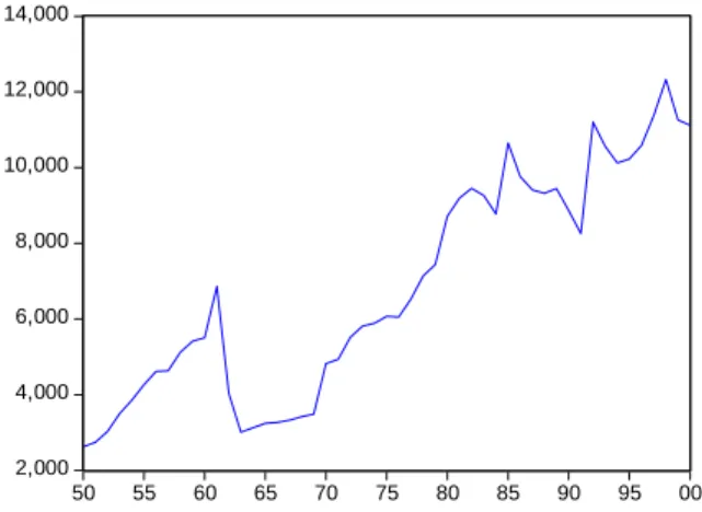
(4) 216. International Journal of Business and Economics. cycle stages are different. GM examined a mature industry where the dynamics have leveled off, but we examine an industry that is probably in a growth stage, as seen in Figure 1. Therefore, we do not expect to find the same model explaining the population dynamics of firms in Turkey. Figure 1. Evolution of Number of Firms in Turkish Manufacturing Industry, 1950-2000 14,000. 12,000. 10,000. 8,000. 6,000. 4,000. 2,000 50. 55. 60. 65. 70. 75. 80. 85. 90. 95. 00. Note that the official statistics for the number of firms include all establishments with power equipment with 10 horsepower or more and establishments with 10 or more persons regardless of power equipment between 1950 and 1962. Only the establishments that employed 10 or more people engaged in the private sector and all establishments in public sector are included between 1963 and 1968 and since 1971. For the year 1970, the inclusion criteria in the official statistics are more than 10 employees or greater than 50 horsepower. As can be observed in Figure 1, the change in the official description seems to have resulted in a sharp decline in the statistics for the year 1962, but a dummy for this year did not appear to be significant in the regressions. Entry and exit dynamics are likely to have long-run repercussions on the market; therefore this study employs annual data, ignoring short-run distortions to capture long-run population dynamics. Since sales data are not available, we use value-added data instead to reflect the size of the market in the simple-form models in (1)-(4). After selecting the appropriate model, we include average payments per employee to reflect the labor cost changes, the ratio of electricity consumption to real value added to represent energy intensity (this is called the mechanization variable and is used as a proxy for capital intensity—see Fotopoulos and Spence, 1999), average number of employees to denote the average firm size, and GDP per capita to control for business cycles. The data are available annually for the period 1950-2000 and were obtained from the Statistical Indicators publication of the State Institute of Statistics in Turkey, except for real GDP per capita, which was obtained from the Penn World Tables. Note that the growth rates of average employment, real GDP per capita, average payments per employee, and energy intensity are computed.

(5) 217. Ugur Soytas. from the data obtained and these growth rates are employed in the regressions. All data are available from the author upon request. The next section presents and discusses the statistical results and compares the four models. 3. Statistical Results and Discussion We first estimate the models as they appear in GM for the Turkish manufacturing industry. The results from the simplest-form models are summarized in Table 1. Table1. Statistical Results based on Simple Forms of the Four Models in GM (i). C. (ii). (iii). N t2−1 ΔN t −1 ΔVAt −1. T T2. T * (T − 1). c. –0.315935 –0.039117 –0.272194 –0.272646. (vi). (vii). (viii). b. 0.343670. 0.369786 (0.24752). – 0.010807 (0.179363) 0.014515 (0.015476) (0.014374) –1.673110 (23.32997) 2.796294 (2.025519) –. –. –. –. –. –. –. – – – –. – 0.004127. 0.257267. 0.520046. (711.004). (0.166787) (0.03092) (0.148794) (0.148512) (0.28133) (0.326620) (0.22906). –0.017470 VAt −1. (v). (574.9944) (190.668) (420.1485) (435.2998) (770.649) (714.5304) (647.478) c. N t −1. (iv). 1382.322b 434.4541b 951.7354b 982.9968b –431.4685 –727.0194 –561.4750 –637.2684. –0.000021 –0.000065b –0.000052a –0.000057a (0.000019) (0.000025) (0.000019) (0.000020) 0.097529. –. –. –. –. –. –. –. –. –. –. –. –. –. –. 25.21391. 22.99716. –. –. –. –. (0.181205). (22.30767) (24.19757) 0.484131. 0.521768. (0.583865) (0.627246) –. – –. –. –. –38.59783 (30.50951) 2.212031b (0.881734) –. (0.14413). 1.475411b 1.612108b (0.65060). (0.66311). F-stat. 1.348234. 0.358878 2.336378c. 1.685540. 1.180132. 4.173049a 5.226779a 3.915627c. R2. 0.161499. 0.019343. 0.132225. 0.132871. 0.047817. 0.270572. 0.254219. 0.262518. Adjusted R 2. 0.041713 –0.001088 0.075631. 0.054041. 0.007299. 0.205734. 0.205582. 0.195475. Notes: ΔN t is the response variable, Δ denotes first difference, N is the number of firms, C is constant, VA is real value added, and T is trend. The subscript t denotes year and superscripts a, b, and c represent significance at 1%, 5%, and 10% levels, respectively. Standard errors are in parentheses and are White heteroscedastic consistent. F-stat is the overall F-statistic of overall significance for the model.. Regressions (vi) and (vii) in Table 1 are the only ones with an overall significance at 1%. Models (iii) and (viii) are only marginally significant. Regression (vi), which is based on the density dependence model, seems to best fit the data. As GM state, the “ N t2−1 term is the distinctive feature of the density dependence model,” and it is significant in (vi). This implies that the population growth rate of firms in the Turkish manufacturing sector is associated with population density. Note that regression (v), which is the density dependence model.

(6) 218. International Journal of Business and Economics. without a time trend is insignificant, whereas introducing trend terms in (vi) seems to make a considerable contribution. Although the coefficient of the linear trend term is not statistically significant, the redundancy of the squared trend term is rejected at a 5% level. GM noted that the density dependence model, frequently used by organizational ecologists, is an Sshaped approach (see Geroski, 2001, for a discussion of the similarities and differences between industrial economics and organizational ecology approaches and Barron, 2001, for a related comment) to modeling the population growth rate. The adjusted R 2 of the selected model does not seem to drop significantly (0.21); hence, the explanatory power cannot be attributed to low sample size relative to the number of regressors. Probably the most important feature of the model is that the quadratic trend term is significant and the effect of N t2−1 seems to be slightly higher than in model (vii). Note that although Şenses and Taymaz (2003, p. 452) indicated 1960 and 1970 as the beginnings of structural changes in the Turkish manufacturing industry, both Chow forecast and breakpoint tests fail to reject the null for 1970 at 1% and 5% respectively (results available upon request). The density dependence model with a quadratic trend is the most suitable for the Turkish manufacturing industry, in contrast with regression (viii) for the US car producers in GM. GM suggested that these models will serve as the basis for more complicated models in the future. Considering other micro or macro variables is out of the scope of their work. In the previous section, we determined that the density dependence model is most appropriate for the Turkish manufacturing industry. Whether the explanatory power of the simplest-form density dependence model may be improved is explored in the next section. 4. Extending the Density Dependence Model In this section, four variables are considered in the extension of the selected model: the growth rates of real GDP per capita, average real payments made to employees, average employment, and electricity consumption per real value added. The full regression model is: ΔN t = β 0 + β1 N t −1 + β 2 N t2−1 + β 3T + β 4T 2 + β 5 RGDPt + β 6 RPAYt + β 7 EMPt + β 8 ELECt + ε t ,. (5). where N is the number of firms, T is trend, RGDP , RPAY , EMP , and ELEC represent growth rates of real GDP per capita, average real payments per employee, average employment, and average electricity consumption per real value added in manufacturing respectively, subscript t indexes years, and ε is the error term. Note, however, that if the series of concern are not stationary, ordinary least squares may yield spurious results. Hence, we employ augmented Dickey-Fuller (1979) (ADF), Phillips and Perron (1988) (PP), Kwiatkowski et al. (1992) (KPSS), Elliot et al. (1996) GLS-detrended Dickey-Fuller (DF-GLS), and Ng and Perron (NP) (2001) unit root tests to examine the stationarity properties of the variables. See.

(7) Ugur Soytas. 219. Maddala and Kim (1998) for an excellent treatment of ADF, PP, KPSS, and DFGLS and Ng and Perron (2001) for NP. For the unit root tests that are sensitive to lag lengths, the results are checked with three different lag selection criteria: Akaike information criterion (AIC), modified AIC, and general to specific t-test methodology. There is no evidence in favor of a unit root in any of the growth rate series (results available upon request). The intuition behind economic growth is clear. Including real GDP per capita growth in the regression is an attempt to control for the business cycles. Economic growth stimulates new entry (this is the “pull hypothesis”). Note however that as the economy contracts, the unemployment rate rises (unemployment rate is commonly used as a proxy for entrepreneurial supply). The microeconomic implication is that the opportunity cost of entry declines. Therefore, a sharp decline in (or a negative) economic growth rate may also have positive effects on the number of firms in an industry (this is the “push hypothesis”) (Ilmakunnas and Topi, 1999). The expected sign of economic growth in the regression is positive, since it is assumed that the pull effect dominates the push effect through time. The lack of capital related data may be partially overcome by the inclusion of electricity consumption per output (Fotopoulos and Spence, 1999). In this model, we employ the growth rate of electricity consumption per real value added instead of changes in capital intensity. Beaudreau (2005) pointed out that the role of energy consumption in production is marginalized in the growth literature, which deviates from the engineering convention of production. He argued that the relationship between energy and production should be accounted for by economists. Indeed, results presented in Sari and Soytas (2004) suggested that energy consumption is more important than labor in explaining the forecast variance of output, and it is almost as explanatory as capital in Turkey. Changes in energy intensity is expected to have a negative effect on population growth rate by discouraging entry and inducing exit since as the growth rate of energy intensity rises, the opportunity cost of staying in that industry also rises. Percentage changes in average employment represent changes in the average firm size. Intuitively, what one expects to observe is a decline in the entry and exit rates (hence a decline in population growth rate) as the growth rate of typical firm size rises. As the growth rate of average firm size exceeds the growth rate of output, the number of firms in the industry declines, a phenomenon referred to as “shakeout” in the literature (see for example Klepper and Graddy, 1990; Jovanovic and Macdonald, 1994; Horvath et al., 2001; Roberts and Thompson, 2003). A brief review of the growth rate of average employment suggests that shakeout occurred in 1962. Therefore, the expected sign of the coefficient of the average firm size growth rate is negative. The growth rate of real average payments to employees represents the annual growth of average wage expenses in the industry. Lay (2003) suggested adding the growth rate of the average wage to account for labor cost effects in Taiwan’s manufacturing sector due to the comparative advantage the country has in labor costs. The inclusion of this variable also allows one to capture the disadvantages due.

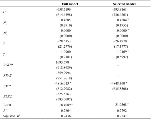
(8) 220. International Journal of Business and Economics. to small firm sizes. Although energy consumption appears to be slightly more important than labor in Turkey (Sari and Soytas, 2004), similar arguments may hold for the Turkish manufacturing industry. The expected sign of the average wage growth rate is negative in the density dependence model, since an increase in the labor cost growth rate may deter entry and induce exit. 5. Estimation Results Table 2 presents results of the full model and the model selected based on the best subsets approach. Table 2. Extending the Density Dependence Model Full model. Selected Model. –658.5196. –595.9161. (614.4498). (436.4261). N t −1. 0.4285 (0.2910). 0.4284 b. 2 t −1. –0.0000 (0.0000). C. N T T. 2. –28.6153. (0.0000) –26.4970. (21.2776). (17.1777). 1.0900 (0.7181). RGDP. RPAY EMP ELEC. F–stat. (0.1955) –0.0000 b. 1093.598 (918.8689) –359.9994 (951.9618) –4816.013 a (812.9082) –325.5563 (583.0007) 18.4089 a. 1.0169 c (0.5992) – – –4848.360 a (635.8508) – 31.0568 a. 2. R 0.7864 0.7792 Adjusted R 2 0.7436 0.7541 Notes: C is constant, N is the number of firms, T is trend, RGDP , RPAY , EMP , and ELEC represent growth rates of real GDP per capita, average real payments per employee, average employment, and average electricity consumption per real value added respectively. Subscript t denotes time and superscripts a, b, and c represent significance at 1, 5, and 10% respectively. Standard errors are in parentheses and are White heteroscedastic consistent. F-stat is the overall F-statistic of overall significance for the model. Diagnostic tests do not reveal serious violations of common assumptions for either model.. The full model is significant at the 1% level based on the overall F-statistic and has a high explanatory power in terms of the adjusted R 2 . Although the signs of the additional variables are as expected, only the coefficient for average employment is.

(9) Ugur Soytas. 221. statistically significant. The population dynamics do not appear to be significantly affected by changes in average labor cost or energy intensity and do not seem to follow the business cycles. Since none of the variance inflation factors is above 5, collinearity does not appear to be a problem. Running the best subsets regression results in a density dependence model that only includes the growth rate of average employment based on both adjusted R 2 and the CP statistic (all unreported statistical results are available upon request). There is a slight improvement in the adjusted R 2 , and the overall F-statistic is higher than that for the full model. Note also that the high explanatory power of the regression cannot be attributed to the overly small sample size relative to the variables included in the regression equation (only a slight downward adjustment from R 2 ). Diagnostic tests conducted on the residuals do not indicate severe violations of the common assumptions, such as normality and parameter stability. Low explanatory power observed in the literature even for panel studies (Geroski, 1995) does not appear to be a problem in this study. The selected regression model also features significant coefficients of all variables, except for T . A significant N t2−1 term indicates nonlinear density dependence; however, its effect appears to be marginal and negative. The number of firms in the previous period ( N t −1 ) seems to have a significant positive impact on the population growth rate, whereas the coefficient for N t2−1 is negative but marginal for small population sizes. The firm number growth rate appears to follow a positive quadratic trend. Average firm size seems to be an extremely important factor driving the population dynamics in a significantly negative fashion. If one can assume that the growth rate of average firm size closely follows a minimum efficient scale, this result should not be surprising. Based on estimation results, the growth rate of population size in the Turkish manufacturing industry depends on a nonlinear density, quadratic trend, and average firm size. 6. Conclusions and Implications for Future Research In this study we examine the dynamics of firm population in the Turkish manufacturing sector and select a model from the four suggested models in GM. Despite data limitations and quality concerns, the density dependence model appears to explain the data reasonably well. Indeed we observe a relatively higher explanatory power than many studies in the literature. One interesting finding may be that business cycles do not appear to play a role in determining changes in firm numbers in the industry. The number of firms is negatively influenced by the average number of employees, which is consistent with the literature on entry and exit; however, it does not appear to depend on average payments to employees. Energy intensity is another factor with no apparent influence on population size dynamics. One major shortcoming in this application is the lack of firm level data. Furthermore, the length of the series we employ is not too long (50 observations as opposed to 93 in GM), and the addition of new variables in the equations rapidly.

(10) 222. International Journal of Business and Economics. depletes the degrees of freedom. Therefore, we have to keep the models as simple as possible. Not only that, but 50 years may not be enough to reflect the entire life cycle of a market. Another problem may be that the data is an aggregate of all the manufacturing industries in Turkey. More specifically classified industries may have different structural changes and population dynamics that may offset each other in the aggregated data. Finally, the quality of the data may also be questioned; however, it is the only data available. Even in the presence of these limitations and problems, the statistical results appear to be robust. In essence, to the extent that longitudinal data is available, a time series investigation of the dynamics of firm population appears to be simple and promising and may complement cross-sectional analysis. However, different manufacturing industries are likely to follow different models of population dynamics. Hence, an interesting and natural extension of this paper may be to use a time series approach in more specifically defined markets. Furthermore, firm-level variables (for example profitability) are absent in the current application because they are not available. Future time series research may benefit from the inclusion of firm-level variables as well as extending the explored industry and macro-level variables. References Amel, D. F. and J. N. Liang, (1997), “Determinants of Entry and Profits in Local Banking Markets,” Review of Industrial Organization, 12, 59-78. Barron, D. N., (2001), “Organizational Ecology and Industrial Economics: A Comment on Geroski,” Industrial and Corporate Change, 10, 541-548. Beaudreau, B. C., (2005), “Engineering and Economic Growth,” Structural Change and Economic Dynamics, 16, 211-220. Caves, R. E., (1998), “Industrial Organization and New Findings on the Turnover and Mobility of Firms,” Journal of Economic Literature, 36, 1947-1982. Dickey, D. A. and W. A. Fuller, (1979), “Distribution of the Estimators for Autoregressive Time Series with a Unit Root,” Journal of the American Statistical Society, 74, 427-431. Disney, R., J. Haskel, and Y. Heden, (2003), “Entry, Exit and Establishment Survival in UK Manufacturing,” The Journal of Industrial Economics, 51, 91112. Doi, N., (1999), “The Determinants of Firm Exit in Japanese Manufacturing Industries,” Small Business Economics, 13, 331-337. Elliott, G., T. J. Rothenberg, and J. H. Stock, (1996), “Efficient Tests for an Autoregressive Unit Root,” Econometrica, 64, 813-836. Fotopoulos, G. and N. Spence, (1999), “Net Entry Behaviour in Greek Manufacturing: Consumer, Intermediate and Capital Goods Industries,” International Journal of Industrial Organization, 17, 1219-1230. Geroski, P. A., (1995), “What Do We Know about Entry?” International Journal of Industrial Organization, 13, 421-440..

(11) Ugur Soytas. 223. Geroski, P. A., (2001), “Exploring the Niche Overlaps between Organizational Ecology and Industrial Economics,” Industrial and Corporate Change, 10, 507-540. Geroski, P. A. and M. Mazzucato, (2001), “Modelling the Dynamics of Industry Populations,” International Journal of Industrial Organization, 19, 1003-1022. Horvath, M., F. Schivardi, and M. Woywode, (2001), “On Industry Life-Cycles: Delay, Entry, and Shakeout in Beer Brewing,” International Journal of Industrial Organization, 19, 1023-1052. Ilmakunnas, P. and J. Topi, (1999), “Microeconomic and Macroeconomic Influences on Entry and Exit of Firms,” Review of Industrial Organization, 15, 283-301. Jovanovic, B. and G. M. MacDonald, (1994), “The Life Cycle of a Competitive Industry,” Journal of Political Economy, 102, 322-347. Kaya, S. and Y. Ucdogruk, (2002), “The Dynamics of Entry and Exit in Turkish Manufacturing Industry,” Middle East Technical University, Economic Research Center Working Papers in Economics, No.02/02. Klepper, S. and E. Graddy, (1990), “The Evolution of New Industries and the Determinants of Market Structure,” RAND Journal of Economics, 21, 27-44. Kwiatkowski, D., P. C. B. Phillips, P. Schmidt, and Y. Shin, (1992), “Testing the Null Hypothesis of Stationarity Against the Alternative of a Unit Root: How Sure Are We That Economic Time Series Have a Unit Root?” Journal of Econometrics, 54, 159-178. Lay, T.-J., (2003), “The Determinants of and Interaction between Entry and Exit in Taiwan’s Manufacturing,” Small Business Economics, 20, 319-334. Maddala, G. S. and I.-M. Kim, (1998), Unit Roots, Cointegration, and Structural Change, Cambridge: Cambridge University Press. Martin-Marcos, A. and J. Jaumandreu, (2004), “Entry, Exit and Productivity Growth: Spanish Manufacturing during the Eighties,” Spanish Economic Review, 6, 211-226. Mathis, S. and J. Koscianski, (1997), “Excess Capacity as a Barrier to Entry in the US Titanium Industry,” International Journal of Industrial Organization, 15, 263-281. Ng, S. and P. Perron, (2001), “Lag Length Selection and the Construction of Unit Root Tests with Good Size and Power,” Econometrica, 69, 1519-1554. Phillips, P. C. B. and P. Perron, (1988), “Testing for a Unit Root in Time Series Regression,” Biometrika, 75, 335-346. Roberts, B. M. and S. Thompson, (2003), “Entry and Exit in a Transition Economy: The Case of Poland,” Review of Industrial Organization, 22, 225-243. Sari, R. and U. Soytas, (2004), “Disaggregate Energy Consumption, Employment and Income in Turkey,” Energy Economics, 26, 335-344. Senses, F. and E. Taymaz, (2003), “Unutulan Bir Toplumsal Amaç: Sanayilesme Ne Oluyor? Ne Olmalı?” in Iktisat Üzerine Yazılar II: Iktisadi Kalkınma, Kriz ve Istikrar, A. H. Köse, F. Senses, and E. Yeldan eds., Iletisim Yayınları: Istanbul..

(12)