Identifying Prototypical Melodies by Extracting Approximate
Repeating Patterns from Music Works
*NING-HAN LIU, YI-HUNG WU+AND ARBEE L. P. CHEN++
Department of Management Information Systems National Pingtung University of Science and Technology
Pingtung, 912 Taiwan
+Department of Information and Computer Engineering Chung Yuan Christian University
Chungli, 320 Taiwan
++Department of Computer Science
National Chengchi University Taipei, 116 Taiwan
The concept of a prototypical melody has been proposed to characterize sets of similar musical segments in a composition. In musicology, the degree of importance as-sociated with a prototypical melody is proportional to the number of musical segments similar to it. In this paper, a novel approach is developed to extract all the prototypical melodies in a musical work. Our approach considers each music segment as a prototypi-cal melody candidate and utilizes edit distance to isolate a set of music segments that are similar to this candidate. To expedite the process, a lower bounding mechanism is used to estimate the number of similar musical segments for each candidate to eliminate im-possible options. Furthermore, the approach is extended to facilitate the extraction of all prototypical melodies in a set of musical works. Analysis is carried out on a real data set, and the results indicate significantly improved performance in average response time relative to existing approaches.
Keywords: prototypical melody, approximate repeating pattern, lower-bounding
mecha-nism, R*-tree, music database
1. INTRODUCTION
The extraction of musical features from the raw data of a composition is fundamen-tal to content-based music retrieval and style analysis. Most classical works of music are composed according to the traditional structures of musical form in which two basic rules are observed: the hierarchical rule and the repetition rule [8]. The hierarchical rule stipulates that compositions are formed hierarchically; a music work consists of
move-ments, a movement consists of sentences, a sentence consists of phrases, and a phrase
consists of figures. The repetition rule maintains that there exist specific sequences of notes, known as motives, repeating in a movement. For example, the well-known motive “G-G-G-Eb” repeatedly appears in Beethoven’s Symphony No. 5. The repetition rule also
manifests in other musical genres such as pop, where the refrain relies heavily on these recurring motives. In previous works [6], a sequence of notes appearing more than once in a composition has been designated as a repeating pattern. In structure and style analy-Received August 11, 2008; revised March 25 & June 17, 2009; accepted July 17, 2009.
sis, there is consensus that repetition is an almost universal characteristic [8, 17]. The short length of repeating patterns, coupled with the ubiquity of this musical feature, lend to their utility in content-based music retrieval, satisfying both efficiency and effective-ness requirements.
The problem of finding all the repeating patterns from a string has been discussed in [5], with suffix-tree based solutions proposed wherein each path of the tree represents a pattern and each leaf node preserves the position of a corresponding pattern located within the string; by traversing the suffix-tree, all repeating patterns can be extracted. These approaches consider the patterns represented by different paths to be distinct. As a result, only precisely repeating patterns can be found. Two approaches based on
correla-tive-matrix and string-join techniques have been proposed by Hsu, Liu and Chen to
ex-tract exact repeating patterns from musical compositions [6]. The former approach en-tails the alignment of notes along the x- and y-axes to form a correlative matrix in order to discern repeating patterns. The latter approach combines shorter repeating patterns into longer ones, and excludes impossible candidates in the process. In the work of Shih
et al. [16] a musical score is segmented into bars, which are further encoded to improve
the efficiency of repeating pattern extraction. Except for the encoding mechanism, the approach also adopts the string-join technique, joining shorter repeating patterns into longer ones.
One the other hand, a pattern may repeatedly appear in a work of music with some variations. A popular approach to coordinating and understanding such variations is rec-ognizing the prototypical melody, which is an abstraction of the composition to which musical segments of similar form correspond [15]. The prototypical melody has a sub-stantial impact on the way melodic structures are memorized by the human brain. Pien-imäki [12] considered musical transposition at length, and adopted a text-mining algo-rithm to extract all the longest unique repeating patterns – those which are not contained in any others. This approach permits the extracted patterns to be discontinuous in the context of a work of music; shorter candidates are initially generated, unqualified options are removed and remaining candidates are combined to form longer patterns. Experi-ments show that the execution time of this approach is considerable due to the large number of candidates to be examined. Rolland [13] proposes a flexible similarity meas-ure for musical segments and a dynamic-programming method for extracting approxi-mate repeating patterns. A musical segment is regarded as a point on a graph, and the similarity between each point is computed. All prototypical melodies are subsequently resolved by counting the number of similar musical segments for each point on the graph. This approach incurs substantial computational overhead in determining the similarity between music segments. Several generalized but efficient algorithms for approximate string matching can be found in [9], and a new search procedure for approximate string matching over suffix trees is proposed in [14].
In this paper, we consider each music segment as a candidate prototypical melody, or approximate repeating pattern (ARP). Two constraints, the maximum and minimum pattern lengths, are set to filter out candidates that are not of interest. For each candidate identified, edit distance and threshold parameters are used to identify all musical seg-ments that are similar to the candidate. Based on the number of similar music segseg-ments and the manner in which they overlap, ARP candidates are either accepted or rejected. Efficiency considerations necessitated the design of a modified R*-tree to exclude
im-possible candidates prior to the computation of edit distances. We adopt a filtering method that uses a distance measure to approximate the edit distance by which the num-ber of segments to be examined for each ARP candidate is reduced. The similar filtering techniques have been presented in the literature [3, 11]. Since it is difficult to ascertain appropriate values for the above constraints and thresholds, an interactive environment is necessary to enable these parameters to be tuned without rerunning the entire process; the modified R*-tree we have developed fulfills this requirement. In addition to these ARP extraction techniques, we consider the approximate repeated pattern in a set of musical compositions (G_ARP) and extend our method to efficiently extract the G_ARP.
The remainder of this paper is organized as follows. In section 2, we define the ap-proximate repeating pattern and formulate the ARP and G_ARP extraction problems. Section 3 delineates our approach to solving these extraction problems, and section 4 presents and discusses experimental results. Finally, section 5 concludes the paper and avenues for future research are exposed.
2. PROBLEM FORMULATION
The problem of prototypical melody extraction has been defined in the work of Rol-land [13], where patterns composed of musical segments are termed star-type patterns. In such a pattern, the single segment to which all others are related over a predefined threshold is referred to as the pivot. This paper regards the pivot as a prototypical melody if it is the origin of a star-type pattern. Several constraints will now be specified in the formulation of our problem.
2.1 Data Representation
Notes in a melodic composition possess two critical properties: pitch and duration. Each note in a symbolic music file (e.g. MIDI) can therefore be represented as a triple (p,
s, e) where p is the pitch value, s is the start time (note on), and e is the end time (note off). As a result, a music file results in an ordered list of triples sorted by the note-on time, i.e. (p1, s1, e1), (p2, s2, e2), …, (pn, sn, en) where s1≤ s2 ≤ … ≤ sn. Two musical pieces
whose notes have matching pitch values are often considered to be the same despite variations in note duration. In light of this, the importance of pitch order supersedes that of precise time intervals. Moreover, since two melodies with the same pitch contours are considered equivalent, the following defined intervals are implemented.
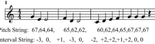
Definition 2.1 Pitch String: A pitch string P = (p1, p2, …, pm) is the ordered list of pitch
values pi, where m is the string length denoted |P| = m.
Definition 2.2 Interval String: An interval string of a pitch string P = (p1, p2, …, pm) is
defined as D = (d1, d2, …, dm-1), where di = pi+1 − pi, 1 ≤ i < m and di is called an interval.
The set of all the distinct interval values in D is denoted ∑D, and size is defined as
|∑D|. Fig. 1 presents examples of a pitch string and an interval string.
Definition 2.3 Interval Segment: An interval segment S[i:j] is the substring of an
Fig. 2. Selected entries of one ricercare (Francesco da Milano: monothematic lute ricercare from the Cavalcanti Lutebook, f. 71v).
Fig. 3. Evolution of diatonic-pitch pattern. Pitch String: 67,64,64, 65,62,62, 60,62,64,65,67,67,67
Interval String: -3, 0, +1, -3, 0, -2, +2,+2,+1,+2, 0, 0 Fig. 1. A pitch string and an interval string.
For simplicity of expression, the terms string and segment are taken to mean
inter-val string and interinter-val segment, respectively. 2.2 Approximate Repeating Patterns
If no constraint is implemented in isolating repeating patterns, superfluous patterns may be extracted and be of little interest to a user due, for instance, to excessive length or brevity. Therefore, we define several constraints to filter out unimportant music patterns as follows.
Overly long segments tend to contain duplicate information, while excessively short segments may not furnish sufficient information pertaining to musical semantics. There-fore, allowing users to specify constraints on pattern length will reduce the unnecessary computational costs associated with the generation of duplicate information or large volumes of very short segments. In this paper, two constraints are imposed on the pattern length: the maximum length (max_len) and the minimum length (min_len). As a result, segments are generated from a given string using a sliding window whose scope is de-fined by min_len and max_len. For example, given a string (a, b, c, d), the qualified seg-ments are (a, b), (b, c), (c, d), (a, b, c) and (b, c, d) when min_len = 2 and max_len = 3. The edit distance [5] is a well known tool in the measurement of melodic similarity [2, 15] and for this reason is adopted in computing the degree of similarity between two seg-ments.
The example in Fig. 2 shows five variants of a prototypical melody produced by edit operations, which are audibly related entries of one ricercare for lute. As shown in Fig. 3, they can be regarded as the stages in the evolution of a diatonic motif through a series of edit operations of total distance 2 [15].
A (meas. 4)
B (meas. 7)
C (meas. 19)
D (meas. 25)
Definition 2.4 Edit Distance: Based on the definition presented in [5], the three types of edit operations that transform segment P (denoted p1, …, pm) into segment Q (denoted q1, …, qn) are insertion, deletion, and replacement. The edit distance between segments P
and Q is the minimum number of edit operations required to transform P into Q, and is denoted edit(P, Q).
The similarity degree between two segments depends on the edit distance, which is normalized between 0 and 1.
Definition 2.5 Similarity Measure: Given two segments P and Q, the similarity
be-tween them is sim(P, Q)= 1 − (edit(P, Q)/max(|P|, |Q|)), where |P| and |Q| are the respec-tive lengths of P and Q.
Definition 2.6 Similar Segments: Given a similarity threshold λ, 0 ≤ λ≤ 1, a segment P is similar to Q if sim(P, Q) ≥ λ.
When two similar segments overlap to a high degree, they can be treated as one segment. To quantify this consideration, we define the overlapping degree as follows.
Definition 2.7 Overlapping Degree: Given two similar segments S[a:b] and S[c:d] where a ≤ c ≤ b, the overlapping degree of is (b − c + 1)/min(b − a + 1, d − c + 1) if b < d. Oth-erwise it is equal to 1.
Since the overlapping degree depends on the segment length, a variable threshold is used to restrict the maximum overlapping degree among the similar segments.
Definition 2.8 Overlapping Threshold: An overlapping threshold for two similar
seg-ments I and J is OIJ = min(|I|, |J|) * ρ , where |I| and |J| are the segment lengths and ρ is
the overlapping threshold ratio, 0 ≤ ρ≤ 1.
Definition 2.9 Extension of a Pivot: Given a pivot P and the set of all similar segments S, an extension of P (denoted Ext(P)) is a subset of S where every pair of segments in it
satisfies the overlapping threshold condition. The number of segments in an extension is called the support, and denoted |Ext(P)|.
For applications in music classification [7], placing a constraint on the minimum number of occurrences for a repeating pattern in a work of music ensures that discovered patterns are of particular significance. In this paper, the constraint on the support of an extension is called the support threshold, and is denoted min_sup.
Definition 2.10 Approximate Repeating Pattern: A pivot P meets the definition of an
ARP if there exists at least one Ext(P) satisfying the support threshold condition, with |Ext(P)| ≥ min_sup.
Definition 2.11 Problem of ARP Extraction: Extract all ARPs for a given musical
string where min_len, max_len, λ, ρ and min_sup are defined.
A particular prototypical melody and its associated segments may appear in multiple compositions, and often multiple times therein. Such familiar melodies (patterns) can be used to establish the character of a work of music, and may enhance appreciation of the
piece by highlighting the composer’s allusion to a recognizable milieu. Moreover, these patterns can be employed in a music classification system [7] to improve performance. The following definitions are relevant to the extraction of such patterns.
Definition 2.12 Count of ARP for a set of music works: For a set of compositions and
an ARP P in a work of music, the count_ARP of P denotes the number of works in which all values of i, |Exti(P)| ≥ min_sup.
Definition 2.13 Global ARP (G_ARP): An ARP P of a work of music is a G_ARP if count_ARP of P is not less than set_min_sup.
Definition 2.14 Problem of G_ARP Extraction: Extract all G_ARPs for a given set of
music strings where min_len, max_len, λ, ρ, min_sup and set_min_sup are defined.
3. ARP EXTRACTION USING A PRUNING STRATEGY
A naïve and time-consuming solution to the ARP extraction problem is to compute the distance between every two segments to find the extension for each segment. In this section, we introduce an approach based on distance approximation and segment index-ing. Initially, we cut a string into a series of segments using sliding windows of various lengths. Each segment is subsequently transformed into a vector in multidimensional space and used to build a modified version of the R*-tree, in which all the segments are indexed. Furthermore, each vector is provisionally regarded as a pivot that triggers a range query on the index tree designed to retrieve any segments containing possible similarities. Finally, for each pivot with an adequate number of returned segments, we compute the relevant edit distances to determine whether it is an ARP.
3.1 Lower-Bounding Distance
Using dynamic-programming based approaches to compute edit distances between strings generally incurs substantial computational overhead. To ameliorate this problem, we define a distance measure that can be efficiently computed. The rationale behind the proposed measure is as follows. From Def. 2.4, the order of values in segments is seen to have a considerable influence on the edit distance and the computational costs associated with its calculation. We therefore ignore the order, and elect to count the number of oc-currences for each distinct value in a segment instead. Given two segments, the differ-ences between such counts can be combined to approximate the edit distance. Moreover, the distance estimated by our alternative measure is proven to be consistently lower than the actual edit distance. Consequently, we can build a lower-bounding mechanism on the index tree to prune all segment distances exceeding a stipulated parameter. Before intro-ducing this measure, we define each segment as follows.
Definition 3.1 Histogram Vector: Let D be a string with ΣD = {a1, a2,…, an}, S be a
segment of D and hkS be the count of ak in S. The histogram vector (abbreviated Hvector)
HV(S) = <h1S, h
2S, …, hnS>.
All segments are represented in terms of their Hvectors, which are scattered over a multidimensional space termed histogram space where each dimension refers to a dis-tinct value in the string and the total number of dimensions is |∑D|.
Definition 3.2 Histogram Distance: We define an insertion to a dimension in the
Hvec-tor as increasing that dimension by one unit. For two segments S1 and S2 of a string D, the
minimum number of insertions on S1 required to make each dimension in HV(S1) larger
or equal to the corresponding value in HV(S2) is calculated as follows.
2 1 2 1 | | 1 2 1 if ( ( ), ( )) , where otherwise D S S S S i i i i i i i h h h h ins HV S HV S d d o Σ = ⎧ − > = = ⎨ ⎩
∑
(1)The distance between the two Hvectors of segments S1 and S2, called the histogram distance (abbreviated Hdistance), is formulated as follows.
HD(S1, S2) = max(ins(HV(S1), HV(S2)), ins(HV(S2), HV(S1))) (2)
The Hdistance is guaranteed to be lower than the edit distance, and this will now be proven.
Lemma 1 Given two strings S1 and S2, HD(S1, S2) ≤ edit(S1, S2).
Proof: Based on Def. 2.4, edit(S1, S2) is equal to the minimum number of edit operations
required to transform S1 into S2. Let need(S1, S2) denote the minimum number of edit
operations on S1 required to make each dimension in HV(S1) equal to the corresponding
one in HV(S2). Obviously, the inequality need(S1, S2) ≤ edit(S1, S2) holds.
Let the variables a and b denote ins(HV(S1), HV(S2)) and ins(HV(S2), HV(S1)),
re-spectively. For the three types of edit operations on S1, an insertion decreases a by 1, a
deletion decreases b by 1, and a replacement decreases both a and b by 1. After need(S1, S2) operations, a and b should each be zero. To minimize the number of edit operations, a replacement that can decrease a and b simultaneously is first considered.
Let the initial values of a and b be A and B, respectively. There are two cases:
Case I: A ≥ B
The maximum number of replacements is B, since b becomes zero earlier than a. After B replacements, a equals A − B, which is the minimum number of insertions re-quired to let a = 0. ∴need(S1, S2) = B + (A − B) = A ⇒ ins(HV(S1), HV(S2)) = A = need(S1, S2) ≤ edit(S1, S2).
Case II: A ≤ B
Similarly, need(S1, S2) = A + (B − A) = B ⇒ ins(HV(S2), HV(S1)) = B = need(S1, S2) ≤ edit(S1, S2) ∴HD(S1, S2) = max(ins(HV(S1), HV(S2)), ins(HV(S2), HV(S1))) ≤ edit(S1, S2).
de-note the two segment lengths. In contrast, the time complexity of Hdistance computation is O(|∑D|), which is independent of the segment lengths. Even if the transformation cost
is included, the time complexity is only O(max(|∑D|, m, n)). In most practical cases, m * n
is larger than |∑D|. As a result, the Hdistance computation is more efficient than the edit
distance computation.
3.2 Index Tree
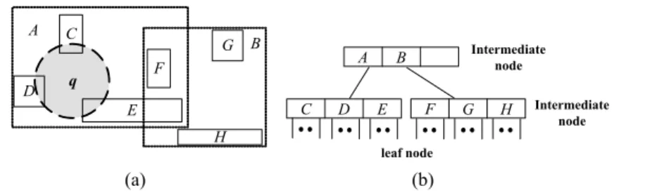
To speed up the retrieval of similar segments for each pivot, we built an R*-tree in the same way as proposed by [1] to index all the Hvectors. An R*-tree uses a multidi-mensional rectangle, called the minimum bounding rectangle (MBR), to represent the data objects in the neighborhood. It is a height-balanced tree composed of leaf nodes and intermediate nodes. A leaf node is associated with the data objects, while an intermediate node keeps the diagonal coordinates of the MBR that encloses its lower level nodes. Fig. 4 shows an example set of data rectangles and the associated R*-tree index. A range query performed on an R*-tree serves to find the data objects located inside the specified region. For example, a range query in Fig. 4 (a) aims at the data located in the region q. All the data represented by MBR B would be pruned as MBR B does not overlap the re-gion q. Therefore, the R*-tree technique speeds up the query processing and guarantees that the pruned data objects are outside the region.
D C F E G H A B A B C D E F G H Intermediate node Intermediate node leaf node q (a) (b)
Fig. 4. (a) Rectangles of an R*-tree and a range query q; (b) R*-tree for the rectangles in (a). Note that other metric access methods [10] including those incorporating cover trees,
k-d trees, m-trees, and vp-trees can also be used in our approach with the same
modifica-tion that is described below.
An interval string is cut into segments by sliding windows according to the two con-straints on segment length. After that, each segment is mapped to a Hvector and inserted into the R*-tree. Each Hvector is inserted into the R*-tree according to its position in histogram space.
Each leaf node in the R*-tree is of the form (I, p-id), where I denotes a minimal bounding rectangle (MBR) and p-id refers to the set of Hvectors contained in I. More-over, each non-leaf node in the R*-tree is of the form (I, child-p), where child-p elements are the pointers of all child nodes and I is the MBR that spans all MBRs of the child nodes. Furthermore, we add entries to each node of the R*-tree such that more nodes can be pruned during tree traversal during ARP extraction. The modified R*-tree is called the
Definition 3.3 RM Pairs: A range in string D is denoted as a:b, where a and b are two
positions in D and a < b. Two segments with ranges a:b and c:d are called non-over-lap-
ping if b < c or d < a, and overlapping otherwise. A set of overlapping segments can then
be represented as (R, M) and termed the RM pair, where R is the union of all their ranges and M is the minimum of their lengths.
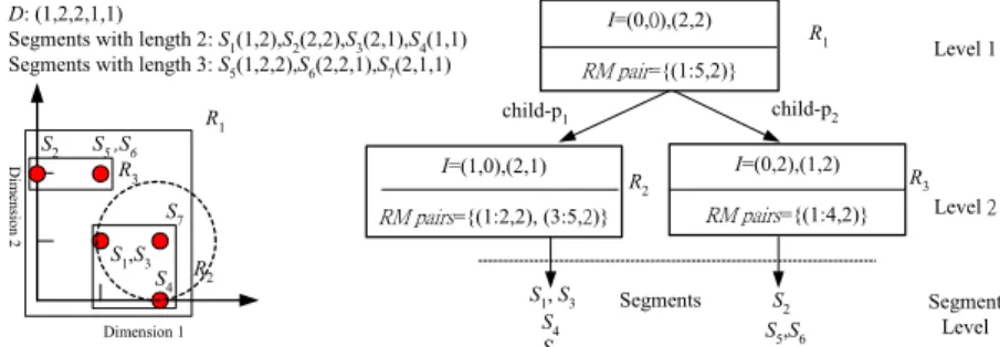
For example, S2(D[2, 3]), S5(D[1, 3]) and S6(D[2, 4]) in Fig. 5 are represented as an
RM pairing (1:4, 2). In the parametric R*-tree, for each node the segments corresponding to Hvectors contained by its MBR are distributed into RM pairs such that the overlapping ones fall into the same RM pair. A parametric R* tree with two leaf nodes and only one non-leaf node is illustrated in Fig. 5. The number of dimensions in the histogram space |∑D| is 2. We construct the parametric R*-tree by sliding windows on D, where min_len
and max_len are set to 2 and 3 respectively. As a result, only two leaf nodes are built to keep all the segments at the bottom level, designated the segment level. For instance, in node R2, the RM pairs are computed in the following manner. Since S7 overlaps S3 and S4,
they form the RM pair (3:5, 2). Conversely, S1 does not overlap any other segment in R2
and therefore the RM pair (1:2, 2) is generated.
D: (1,2,2,1,1)
Segments with length 2: S1(1,2),S2(2,2),S3(2,1),S4(1,1)
Segments with length 3: S5(1,2,2),S6(2,2,1),S7(2,1,1)
Dimension 1 Di men sio n 2 R1 R3 R2 S4 S1,S3 S7 S5 ,S6 I=(0,0),(2,2) RM pair={(1:5,2)} S1, S3 S7 S5,S6 S2 R1 child-p1 child-p2 I=(1,0),(2,1) RM pairs={(1:2,2), (3:5,2)} R2 I=(0,2),(1,2) RM pairs={(1:4,2)} R3 Segments Level 1 Level 2 S2 S4 Segment Level
Fig. 5. An example of the histogram space and a parametric R*-tree.
3.3 ARP Extraction Procedure
In this subsection, our approach to ARP extraction applied to a composition is in-troduced. The algorithm employed entails three main stages. The first stage constructs the parametric R*-tree as an index tree for the next procedure in which we regard each Hvector in the index tree as a range query, which are executed to generate ARP candi-dates. The candidates are recorded as a linked list named CandidateList, which is fed into the final stage. As a result, ARPs satisfying all the stipulated constraints are output. The last two stages are repeated until the ARPs are determined to the user’s satisfaction.
3.3.1 Candidate generation
After index construction, we regard each segment in it as a pivot and use its Hvector as a range query on the parametric R*-tree. Eligible segments of sufficient similarity to the pivot are then returned and designated as candidate segments. Each time a query is processed, the corresponding pivot is pruned if the maximum number of returned results
is less than min_sup. A pivot that survives this query processing is established as a
can-didate ARP. For each cancan-didate, component segments are further analyzed to determine
whether it is an ARP.
Given the Hvector of pivot p (denoted Vp), we retrieve associated candidate
seg-ments from the index tree to decide whether Vp is an ARP candidate in five steps: Step 1: Range query formulation
We need to construct a range query to prune the segments dissimilar to p, so the ra-dius of a sphere in histogram space for Vp (at the center of the range query) must be
de-cided first.
The radius δp is computed as follows.
(1 )*| | , p p λ δ λ − ⎢ ⎥
= ⎢⎣ ⎥⎦ where λ is similarity threshold. (3)
This formula comes from the definition of similar segments. For the pivot p, the inequal-ity sim(p, q) ≥ λ should hold true when q is a similar segment to p. There are two cases to be considered.
Case I: |q| ≥ |p|
From the definition of similarity measurement, the following is obtained.
sim(p, q) = 1 − edit(p, q)/max(|q|, |q|) ≥ λ ⇒ edit(p, q)/|q| ≤ 1 − λ
∵ |q| − |p| ≤ edit(p, q), ∴ (|q| − |p|)/|q| ≤ 1 − λ ⇒ |q| ≤ |p|/λ ⇒ |q| − |p| ≤ (1 − λ) * |p|/λ
The inequality establishes an upper bound on the length of a similar segment that is pro-portional to the length of a given pivot. Moreover, the difference between the lengths of
p and q is lower than or equal to (1 − λ) * |p|/λ.
Case II: |q| ≤ |p|
In the same manner, the inequality |q| ≥ λ * |p| is established. This implies that the
length of a similar segment also has a lower bound. Moreover, the upper bound on the difference between the lengths of p and q is (1 − λ) * |p|.
Since λ is not larger than 1, the value of (1 − λ)*|p|/λ is guaranteed to be larger than or equal to (1 − λ) * |p|. Hence, we use the upper bound as the radius of a range query because it ensures that segments with Hvectors outside the sphere are dissimilar.
Step 2: MBR retrieval
Given the range query with defined parameters (Vp, δp), when traversing a level of
the index tree, all MBRs overlapping with the specified region are retrieved and denoted as overlapping MBRs. The overlapping MBRs of (<2, 1>, 1) presented in the histogram space of Fig. 5 as an example are R1 and R2, located respectively on levels 1 and 2.
Step 3: Estimation for the maximal number of similar segments
For each overlapping MBR, the maximum number of similar segments in it can be estimated in three steps. Firstly, for each RM pair (RX, MX) in the MBR, the minimum
length of segments covered by RX is MX. On the other hand, the length of a similar
seg-ment for p must be at least |p| − δp. Therefore, the minimum length of similar segments
covered by the RM pair (MLX) must be not lower than the maximum of these two lower
bounds, such that max(|p| − δp, MX). Secondly, for each RM pair in the MBR, the
maxi-mum number of similar segments covered by RX is estimated by considering that any two
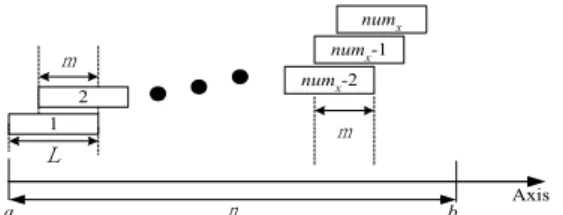
similar segments must satisfy their overlapping thresholds. Referring to the range from a to b on the axis in Fig. 6, we draw a line of length L starting at position a. Another line of the same length is drawn to the right of a such that the length of its overlap with the pre-vious line is equal to m. This process is repeated until a line touches position b. The total number of lines drawn in this way is equal to ⎣(n − L)/(L − m)⎦ + 1, where n = b − a + 1, and is denoted seg_numX; this corresponds to the number of segments with the minimum
length MLX covered by RX if L is set to MLX and m is set to ρ * MLX. Note that ρ is the
overlapping threshold ratio, and thus m is equivalent to the overlapping threshold for any two similar segments in RX. At last, the values estimated for all RM pairs in an MBR are
summed to give the maximum number of similar segments that can be retrieved from the MBR (denoted seg_numMBR). m 1 2 numx numx-1 L numx-2 m Axis a n b
Fig. 6. Maximum number of segments fitted into a range.
For illustration purposes, we will continue to use the example presented in Fig. 5. Suppose that the pivot is S7, ρ is set to 0.5 and the range query (<2, 1>, 1) is performed
on R2. There are two RM pairs, (1:2, 2) and (3:5, 2), in R2. For the former, ML1 = max(3
− 1, 2) = 2, m = ρ * ML1 = 0.5 * 2 = 1 and seg_num1 = ⎣(2 − 2)/(2 − 1)⎦ + 1 = 1. Using
the same formula, the seg_num2 value of the latter is 1 and the seg_numR2 value
com-puted is therefore 2.
Step 4: Candidate pruning before Hdistance computations
When a range query is processed at a level above the segment level, the seg_numR
of each overlapping MBR R is computed and their sum is denoted max_seg_num. To the pivot corresponding to the Hvector Vp, when max_seg_num for the range query (Vp, δp) is
less than min_sup, the pivot cannot be an ARP according to Def. 2.10. In this case, we terminate the processing of this query and return to execute the next range query. If
max_seg_num is not less than min_sup, the given query is recursively propagated
through the lower levels. For example, if we assume that min_sup is set to 3, segment S7
can be pruned because according to the result generated in step 3, the max_seg_num value at level 2 is only 2.
Step 5: Candidate pruning after Hdistance computations
Hdis-tances between the pivot p and the segments whose lengths are not less than min_len and not larger than max_len in the overlapping MBRs. All the segments whose Hdistances satisfy δp are extracted to compute max_seg_num. If max_seg_num is less than min_sup,
the pivot will be pruned. Otherwise, the pivot is regarded as an ARP candidate and the extracted segments are its candidate segments.
After all range queries have been performed, a set of ARP candidates are obtained and their candidate segments are stored in CandidateList, which will be processed further in the final stage.
3.3.2 ARP extraction
The output of our approach includes each ARP and its extensions, which can be used by musicians to verify whether the ARP is a prototypical melody. Given an ARP candidate and its associated segments, the relevant edit distance is computed and candi-date segments violating the distance threshold are removed to isolate a set of similar segments. Subsequently, we generate all the extensions of the ARP candidate by consid-ering the overlapping threshold. If the support of an extension is less than the min_sup, the extension is not a valid solution. Consequently, by Def. 2.10, an ARP candidate is only viable if one of its extensions satisfies the min_sup threshold.
3.4 G_ARP Extraction Procedure
A naïve method for the extraction of G_ARPs from a set of compositions is pre-sented in the following subsection. Parametric R*-trees are built for each composition, and all the pivots that are identified as ARPs are extracted by employing the method pre-viously delineated. For each of the extracted ARPs, we examine its extensions (the sets of similar segments) in other works of music in the set. The number of musical works satisfying the condition provided by Def. 2.12 is computed, and compared against the
set_min_sup value to determine whether the pivot is a G_ARP. Repeating the procedure
until each pivot is characterized will extract all the G_ARPs.
This naïve method is space-consuming because each musical work needs its own tree for indexing. Moreover, individually traversing these trees is time-consuming and computationally exhaustive. We reduce the associated costs by modifying our approach for ARP extraction to enable the G_ARP extraction using only one parametric R*-tree. Let D = {D1, D2, …, Dn} be a set of compositions. For all Di in D, we build a parametric
R*-tree with |∪∑Di| dimensions which is the number of distinct intervals in D required to
index all the segments of Di; the previous subsection describes the procedure for building
this index tree.
We subsequently attach a number (ID) to the R field (the union of all ranges for the overlapping segments) of the RM pair to identify the works to which these segments be-long. As a result, the RM pair takes the form (ID: position1: position2, length). For ex-ample, two segments, S2
2(2, 2) and S23(1, 2, 2), of composition D2 are represented as the
RM pair (2:1:3, 2).
For G_ARP extraction, we modify and enhance the candidate generation procedure of subsection 3.3.1 to facilitate more efficacious exclusion of pivots constituting impos-sible candidates. Originally, step 2 of this candidate generation stipulated retrieval of all
the overlapping MBRs of (Vp, δp). In this enhanced version, an additional step is invoked
to compute the number of distinct IDs in all the overlapping MBRs (denoted ID_nums). Use of the ID_nums value restricts the maximum number of compositions that may con-tain an extension of Vp; a pivot cannot be a G_ARP candidate if ID_nums < set_min_sup,
and is skipped if this fail-condition is satisfied. After step 3, the maximum number of similar segments (seg_numR) is estimated for each overlapping MBR R.
In steps 4 and 5 of candidate generation, we also incorporate several pruning tech-niques. If a pivot is regarded as an ARP after the scrutiny prescribed in subsection 3.3.1,
seg_numR values corresponding to similar segments with the same ID among the
over-lapping MBRs are summed and denoted max_seg_numID. The number of distinct IDs
satisfying max_seg_numID ≥ min_sup is then computed and used as an upper bound on
the count_ARP. The ARP is pruned if this upper bound is less than the set_min_sup value. To circumvent unnecessary computations in step 3, RM pairs with IDs whose associated
max_seg_numID is less than min_sup are ignored during subsequent query processing at
the lower levels.
4. PERFORMANCE EVALUATION
Performance was analyzed in terms of both efficiency and effectiveness. The dataset comprises 2000 MIDI files of classical music from a range of composers, downloaded from various web sites. On average, there are 2953 intervals and 18.7 distinct intervals in a musical work.
4.1 Efficiency Experiment Settings
Many algorithms exist to solve the problem of approximate string matching with good efficiency [9]. However, our method emphasizes a pruning strategy which mini-mizes unnecessary edit distance computations by imposing constraints on key musical properties such as length and count. Calculation of edit distance is the final stage in our method, and is not the main focus of our research; any strategy that improves edit dis-tance computation may be incorporated into our approach. We therefore restrict com-parisons of our method to a modified version of the dynamic-programming approach named FIExPat [13], widely recognized in the field of prototypical melodies extraction. The experimental settings were established as follows. The user defines an initial set of constraints, and the system executes one complete process of ARP extraction (a single
iteration). In each experiment, a single constraint is varied to determine its influence on
the time elapsed during a distinct computational iteration.
4.2 Efficiency Experiment Results
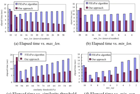
In Fig. 7, the time elapsed is divided into two parts for a single computational itera-tion utilizing our approach. The hashed poritera-tion of the illustraitera-tion represents the comput-ing time for parametric R*-tree construction and pruncomput-ing steps, and the solid portion the computing time for edit distance. With the exception of the first iteration, it is clear that the former is a more rapid computation.
0 2 4 6 8 10 12 14 10 12 14 16 18 20 22 24 26 28 30 max_len (interval number)
el ps ed ti m e (s ec ) FIExPat algorithm Our approach 0 2 4 6 8 10 12 14 16 20 18 16 14 12 10 8 6 4
min_len (interval number)
el ps ed t im e ( sec ) FIExPat algorithm Our approach
(a) Elapsed time vs. max_len. (b) Elapsed time vs. min_len.
0 5 10 15 20 99 94 89 84 79 74 69 64 59 54 49 similarity threshold (%) el ap se d t im e ( sec) FIExPat algorithm Our approach 0 2 4 6 8 10 12 14 16 18 10 9 8 7 6 5 4 3 2 min_sup el ps ed ti m e (s ec) FIExPat algorithm Our approach
(c) Elapsed time vs. similarity threshold. (d) Elapsed time vs. min_sup. Fig. 7. Experiment results.
Fig. 7 (a) illustrates the results for various values of max_len, where the parameters
min_len, min_sup, and λ are set respectively to 4, 5, and 75%. At the first iteration, both
approaches require substantially more time than for all subsequent iterations since our approach must build the relevant parametric R*-tree, and FIExPat must construct the graph structure upon which it relies. Under the implemented constraint variations, our approach performs better than FIExPat over all iterations, and the observed elapsed time decreases as the max_len increases. The reason is that segments with larger lengths are less likely to constitute a similar segment, and can therefore be pruned by our approach. The results for various values of min_len are shown in Fig. 7 (b), where the parameters
max_len, min_sup, and λ are set respectively to 30, 5, and 75%. Here our approach again
consistently performs better than FIExPat, except for the first iteration. The elapsed times for both approaches increase as the min_len decreases, because a smaller min_len means more segments need be considered. If we accumulate the elapsed times over the first and the second iterations for each approach, our approach outperforms FIExPat. This sug-gests that our approach is more suitable than FIExPat in an interactive environment.
In Fig. 7 (c), the results for various values of λ, where the parameters max_len,
min_len and min_sup are set respectively to 30, 4 and 5 are presented. Under this
ar-rangement, the user may loosen the similarity threshold in order to resolve more ARPs. Once again our approach requires more time for the first iteration, but significantly less time for the subsequent iterations. The reason is that our approach builds the parametric R*-tree only at the first iteration, and does not update the index tree at subsequent itera-tions since the max_len and min_len remain unchanged.
Fig. 7 (d) indicates the results generated for various values of min_sup, where the parameters max_len, min_len, and λ are set respectively to 30, 10, and 75%. Our
ap-proach is clearly demonstrated to outperform FIExPat over all iterations.
Figs. 7 (b) and (c), the results in Figs. 7 (a) and (d) show that the time consumed or the linear increase of computation time can be reduced. The reduction of our method is more significant when the parameter max_len is enlarged or the parameter min_sup is de-creased. Therefore, our method is preferable for ARP extraction.
0 50 100 150 200 250 300 350 5 10 15 20 25 number of musicworks el ps ed ti m e ( sec ) FIExPat algorithm ARP algorithm
Fig. 8. Elapsed time vs. number of compositions.
In the experiment regarding G_ARP extraction, the defined constraints include set_
min_sup. The test data pool was compiled by randomly selecting works of music from
our database. Fig. 8 shows the elapsed time for computations involving various numbers of compositions, where the parameters max_len, min_len, and min_sup are set respec-tively to 30, 15, and 5. The parameter set_min_sup is set to 30% of the compositions in the test data, and the elapsed time is defined as the average of three execution times un-der the different values of λ (90%, 80%, and 70%). As the number of musical works in
the database increases, the elapsed time of FIExPat grows rapidly, but the elapsed time of our approach does not. The reason for this is that the time complexity of FIExPat is up-per-bounded by the square of the number of musical works in a database, while our ap-proach avoids superfluous computation of edit distances by imposing the set_min_sup constraint.
4.3 Effectiveness Experiment Results
Due to the absence of standard testing procedures for prototypical melodies and the subjective nature of approximate repeating pattern characterization, only the average ratios of interesting patterns relative to extracted ARPs and G_ARPs are tested for the consideration of a user. Five music professionals were invited to join the study, and each subject selected a unique volume of familiar compositions for testing. After gaining an understanding of the thresholds settings, subjects were asked to indicate whether a given extracted pattern is interesting and the results are shown in Table 1. The ratio of interest-ing patterns extracted from the sinterest-ingle work of music is higher than for a set of composi-tions, likely because the style of music across compositions can vary dramatically and reduce the chance of harmonic patterns. However, all users agree that the tool is useful in the analysis of music.
Table 1. Experimental results for effectiveness.
Average ratio of interesting patterns ARP extraction from single composition 83.2%
G_ARP extraction from set of compositions 67.4%
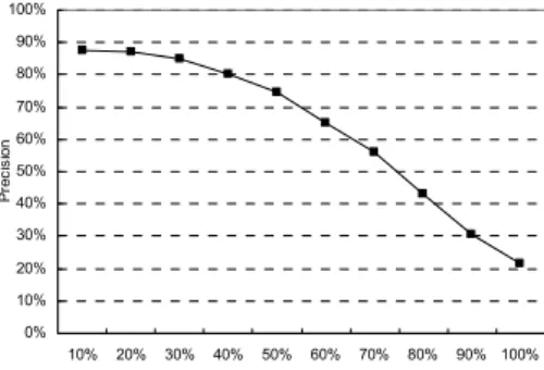
The results of the previous experiments are shown as the precision/recall curve per-taining to the extraction of prototypical melodies. In particular, thirty edit-distance based prototypical melodies of classic musical works are annotated by five music professionals. It can be noted that, in general, when thresholds are adequately assigned (e.g., decreasing the similarity threshold or increasing max_len), we can obtain a high percentage of the predefined prototypical melodies (i.e., high recall). However, the percentage of the pre-defined prototypical melodies among the extracted ones decreases (i.e., low precision). The curve is shown in Fig. 9, implying that if a huge amount of prototypical melodies are sought, a significant number of useless patterns will be produced. It will be interesting to look into this problem for further improvement of our method.
0% 10% 20% 30% 40% 50% 60% 70% 80% 90% 100% 10% 20% 30% 40% 50% 60% 70% 80% 90% 100% Recall P re cis io n
Fig. 9. The precision/recall curve for the extraction of prototypical melodies.
5. CONCLUSION
Since the approximate repeating pattern can be found in both classical and pop mu-sic, it plays an important role in the description of music and analysis of musical styles. In this paper, we develop a novel approach for extracting approximate repeating patterns from musical compositions. This approach adopts the techniques of range query essing for multidimensional data and a special mechanism for reducing the query proc-essing time. In the performance study, the execution time of our approach is significantly reduced relative to the FIExPat approach. Our approach may also be applied in other fields including pattern extraction on web click strings, or DNA strings.
Several potential avenues for further research may be identified. Improving the Hdistance measure to facilitate more efficacious pruning of impossible candidates prior to computation of edit distances will result in substantially more efficient extraction of ARPs and G_ARPs. A sophisticated dimension reduction strategy might be employed to reduce query processing time, and would have a particularly large impact on G_ARP extraction for large databases. Other applications of approximate repeating pattern isola-tion will be investigated as they pertain to music classificaisola-tion, analysis, and retrieval.
REFERENCES
1. N. Beckmann, H. P. Kriegel, R. Schneider, and B. Seeger, “The R*-tree: An efficient and robust access method for points and rectangles,” in Proceedings of the ACM
SIGMOD International Conference on Management of Data, 1990, pp. 322-331.
2. E. Cambouropoulos, M. Crochemore, C. Iliopoulos, M. Mohamed, and M. F. Sagot, “A pattern extraction algorithm for abstract melodic representations that allow par-tial overlapping of intervallic categories,” in Proceedings of the 6th International
Conference on Music Information Retrieval, 2005, pp. 167-174.
3. W. I. Chang and E. L. Lawler, “Sublinear approximate string matching and biologi-cal applications,” Algorithmica, Vol. 12, 1994, pp. 327-344.
4. R. Clifford and M. Christodoulakis, “A fast, randomized, maximal subset matching algorithm for document-level music retrieval,” in Proceedings of the 7th
Interna-tional Conference on Music Information Retrieval, 2006, pp. 150-155.
5. D. Gusfield, Algorithms on Strings, Trees, and Sequences: Computer Science and
Computational Biology, Cambridge University Press, New York, 1997.
6. J. L. Hsu, C. C. Liu, and A. L. P. Chen, “Discovering non-trivial repeating patterns in music data,” IEEE Transactions on Multimedia, Vol. 3, 2001, pp. 311-325. 7. C. R. Lin, N. H. Liu, Y. H. Wu, and A. L. P. Chen, “Music classification using
sig-nificant repeating patterns,” in Proceedings of the International Conference on
Da-tabase Systems for Advanced Applications, 2004, pp. 506-518.
8. E. Narmour, The Analysis and Cognition of Basic Melodic Structures, The Univer-sity of Chicago Press, Chicago, 1990.
9. G. Navarro, “A guided tour to approximate string matching,” ACM Computing
Sur-veys, Vol. 33, 2001, pp. 31-88.
10. C. Parker, A. Fern, and P. Tadepalli, “Learning for efficient retrieval of structured data with noisy queries,” in Proceedings of the 24th International Conference on
Machine Learning, 2007, pp. 729-736.
11. S. Pauws, “Cubyhum: A fully operational query by humming system,” in
Proceed-ings of the International Conference on Music Information Retrieval, 2002, pp. 187-
196.
12. A. Pienimäki, “Indexing music databases using automatic extraction of frequent phrases,” in Proceedings of the International Conference on Music Information
Re-trieval, 2002, pp. 25-30.
13. P. Y. Rolland, “FIExPat: Flexible extraction of sequential patterns,” in Proceedings
of the International Conference on Data Mining, 2001, pp. 481-488.
14. L. M. S. Russo, G. Navarro, and A. L. Oliveira, “Indexed hierarchical approximate string matching,” in Proceedings of the International Conference on String
Proc-essing and Information Retrieval, 2008, pp. 144-154.
15. E. Selfridge-Field, Melodic Similarity: Concepts, Procedures, and Applications (Com-
puting in Musicology: 11), the MIT Press, MA, 1998.
16. H. H. Shih, S. S. Narayanan, and C. C. J. Kuo, “Automatic main melody extraction from MIDI files with a modified Lempel-Ziv algorithm,” in Proceedings of the
In-ternational Symposium on Intelligent Multimedia, Video and Speech Processing,
2001, pp. 9-12.
An Analysis-by-Synthesis Study of Musical Performance, Representing Musical Stru- cture, Academic Press, London, 1991.
Ning-Han Liu (劉寧漢) received a Ph.D. degree in
Com-puter Science from National Tsing Hua University, Taiwan, in 2005. He is an Assistant Professor of the Department of Manage-ment Information Systems, National Pingtung University of Sci-ence and Technology, Pingtung, Taiwan since 2006. His research interests include multimedia databases, audio processing in WSN, and artificial intelligence.
Yi-Hung Wu (吳宜鴻) received a Ph.D. degree in Computer
Science from National Tsing Hua University in 2001. He was a postdoctoral research fellow at National Tsing Hua University in 2001-2006, and joined the Department of Information and Com-puter Engineering, Chung Yuan Christian University, as an assis-tant professor since 2006. His current research interests are in the area of data mining, with emphasis on data stream analysis and applications.
Arbee L. P. Chen (陳良弼) received a Ph.D. in Computer
Engineering from University of Southern California in 1984. He was a professor at National Tsing Hua University from 1991-2004, and is currently Chengchi University Chair Professor and Dean of College of Science at National Chengchi University. He was a vis-iting scholar at Stanford University, King’s College London, and Harvard University. His current research interests include data stream management, multimedia databases, and data mining.