基於H.264視訊編碼在畫面略過轉換下之區塊模式決定與移動向量預測

國

立

交

通

大

學

資訊科學與工程研究所

碩

士

論

文

基 於 H . 2 6 4 視 訊 編 碼 在 畫 面 略 過 轉 換 下

之 區 塊 模 式 決 定 與 移 動 向 量 預 測

Block Motion Decision and Motion Vector Composition

in H.264 Video Frame skipping Transcoding

研 究 生：李威邦

指導教授：蔡文錦 教授

基 於 H.264 視 訊 編 碼 在 畫 面 略 過 轉 換 下

之 區 塊 模 式 決 定 與 移 動 向 量 預 測

Block Mode Decision and Motion Vector Composition

in H.264 Video Frame Skipping Transcoding

研 究 生：李威邦 Student：Wei-Bang Li

指導教授：蔡文錦 Advisor：Wen-Jiin Tsai

國 立 交 通 大 學

資 訊 科 學 與 工 程 研 究 所

碩 士 論 文

A Thesis

Submitted to Institute of Computer Science and Engineering College of Computer Science

National Chiao Tung University in partial Fulfillment of the Requirements

for the Degree of Master

in

Computer Science

June 2008

Hsinchu, Taiwan, Republic of China

基於 H.264 視訊編碼

在畫面略過轉換下之區塊模式決定與移

動向量預測

學生 : 李威邦

指導教授 : 蔡文錦 教授

國立交通大學

資訊科學與工程研究所

摘 要

近年來，許多應用如即時線上播放系統、視訊會議、手持式多媒體、網路媒 體快速瀏覽等需求大量提升。使用者期望在有限的網路傳輸速率以及既有的硬體 設備下，能夠接收高品質的視訊畫面；而系統開發者除了追求能將高畫質的視訊 影片，能以較低的位元壓縮率傳輸外，尚能提供流暢地視訊快速播放閱覽的功能。 在這篇論文當中，我們提出了一個適用於 H.264/AVC 視訊壓縮編碼標準下， 利用畫面省略的轉換編碼方式來降低傳輸位元大小以及所需的視訊壓縮時間。其 中的議題包含在省略畫面的情形下如何解決區塊分割大小模式的決定、區塊移動 向量計算方法。 由實驗的結果可知，我們所提出的方法相較於 H.264/AVC 畫面略過的壓縮以 及其他方法，在維持一定的視訊品質之下，大量的縮減壓縮的時間，並亦能傳輸 於在低位元傳輸率中。 關鍵字：畫面略過轉換、區塊模式決定、移動向量計算

Block Mode Decision and Motion Vector Composition

in H.264 Video Frame Skipping Transcoding

Student: Wei Pang Lee

Advisor: Dr. Wen-Jin Tsai

College of Computer Science

National Chiao Tung University

Abstract

In recent years, many multimedia applications such as real-time video streaming

systems, videoconference, handheld media systems, and high-speed video browsing

through networks are required. Users expect to receive high quality of video under

limited network bandwidth and established hardware equipments. Oppositely, system

providers pursue services of high video quality through low bit-rate transmission in

order to reduce the cost and provide more services.

In this thesis, we focus on a frame-skipping transcoding methods to reduce the

bit-rate for H.264/AVC video coding. We have proposed block mode decision

methods, motion vector composition methods for frame-skipping transcoding.

Experimental results show that, compared with H.264/AVC and other algorithms,

the proposed methods can save a lot of computational cost. The performance can be

improved by maintaining visual quality at low bit-rate.

Table of Contents

CHAPTER 1 INTRODUCTION...1

MOTIVATION...4

CHAPTER 2 BACKGROUND AND RELATED WORK ...5

2.1H.264/AVC ...5

2.2VIDEO TRANSCODING...8

2.3MOTION VECTOR COMPOSITION... 11

CHAPTER 3 THE PROPOSE METHOD ...16

3.1SYSTEM ARCHITECTURE...16

3.2PROPOSED BLOCK MODE DECISION METHOD...18

3.3PROPOSED MOTION VECTOR COMPOSITION METHOD...22

3.3.1 Enhanced FDVS Method for H.264/AVC ...23

3.3.2 Enhanced ADVS Method for H.264/AVC ...26

3.4MVSELECTIONS FOR MODE CHANGE AND NO MODE CHANGE...28

3.5APPLY MOTION VECTOR COMPOSITION...29

CHAPTER 4 EXPERIMENTAL RESULTS...31

4.1FDVS,ADVS, AND PADVS(N)METHODS ON LARGE BLOCK SIZES...32

4.2PROPOSE METHODS ON ALL BLOCK SIZES...35

4.3MVSELECTIONS FOR MODE CHANGE AND NO MODE CHANGE...39

CHAPTER 5 CONCLUSION...41

REFERENCE ...42

APPENDIX A...43

APPENDIX B...47

List of Figures

FIG.1-1BASIC TRANSCODING ARCHITECTURE...2

FIG.2-1H.264/AVCENCODER...6

FIG.2-2VARIABLE BLOCK SIZE IN H.264/AVC ...7

FIG.2-3COMPUTATION OF RDCOST...7

FIG.2-4FRAME SKIPPING TRANSCODER IN PIXEL DOMAIN...10

FIG.2-5BLOCK MATCHING MOTION ESTIMATION ALGORITHM...12

FIG.2-6INTERPOLATION OF MOTION VECTORS...12

FIG.2-7MOTION VECTOR COMPOSITION...13

FIG.2-8BACKWARD MVCOMPOSITION:MVC=MV1+MV2+MV3...14

FIG.2-9FDVSCOMPOSITION SCHEME...14

FIG.2-10ILLUSTRATION OF THE ADVSALGORITHM...15

FIG.3-1PROPOSED H.264/AVC VIDEO FRAME SKIPPING TRANSCODING ARCHITECTURE...16

FIG.3-2FLOWCHART OF PROPOSED BLOCK MODE AND MVDECISION METHODS...18

FIG.3-3DIVIDE INTER BLOCK...20

FIG.3-4FLOWCHART OF MODE DECISION...21

FIG.3-5VARIABLE BLOCK MODE...21

FIG.3-6MODE CHANGE RESULT...22

FIG.3-7AN INTER 4X4FDVSUNIT...23

FIG.3-8(A)FDVS EXAMPLE (B)ORIGINAL FDVS METHOD (C)ENHANCED FDVS METHOD...25

FIG.3-9ENHANCED FDVSEXAMPLE RESULT...26

FIG.3-10AN 4X4INTER ADVSUNIT...27

FIG.3-11SMB8X4,SMB4X8,SMB8X8CHECK ENDPOINT...27

FIG.3-12APPLY ADVSEXAMPLE...28

FIG.3-13MV SELECTIONS FOR (A) MODE CHANGE AND (B) NO MODE CHANGE...29

FIG.3-14APPLY MOTION VECTOR COMPOSITION...30

FIG.4-1DIFFERENT METHODS IN PSNRFRAME BY FRAME IN FOREMAN...34

FIG.4-2COMPARISON ENCODING TIME WITH TRANSCODING TIME FRAME BY FRAME IN FOREMAN...35

FIG.4-3BIT-RATE OF DIFFERENT METHODS IN FOREMAN...38

FIG.4-4BIT-RATE OF DIFFERENT METHODS IN NEWS...38

List of Tables

TABLE 3-1RULES OF MODE CHANGE...20

TABLE 4-1EXPERIMENTAL RESULTS OF FDVS,ADVS AND PADVS(N) ON FOREMAN.CIF...33

TABLE 4-2PROPOSE METHODS COMPARING TO H.264(FOREMAN)...36

TABLE 4-3PROPOSE METHODS COMPARING TO H.264(NEWS) ...36

TABLE 4-4PROPOSE METHODS COMPARING TO H.264(HALL)...36

TABLE 4-5BIT-RATE OF PROPOSE METHODS COMPARING TO H.264 ...37

TABLE 4-6COMPARING MODE CHANGE WITH NO MODE CHANGE IN FOREMAN...39

TABLE 4-7COMPARING MODE CHANGE WITH NO MODE CHANGE IN NEWS...39

Chapter 1 Introduction

The video coding standard MPEG-4 Part10 AVC/H.264 [1] was developed by the

joint video team (JVT) of ISO/IEC (MPEG) and ITU-T (VCEG). The video coding

standard is based on traditional hybrid coding scheme but with several additional

methods to attain high coding efficiency such as adaptive motion compensation with

variable block sizes, multiple reference frames, intra coding with various spatial

prediction directions, and so on. The new technologies mentioned above are quite

important to many networked multimedia services such as multipoint video

conferencing, distance learning, video on demand, and digital TV. Transmission of

compressed video over heterogeneous networks with different transmission

bandwidths may require a reduction in bit rate.

The compressed video bit stream is often converted to the reduced frame rate

video bit stream in order to reduce the bit rate. Video transcoding provides not only

the format conversion but also resolution scaling (spatial transcoding), bit-rate

conversion (quality transcoding), and frame rate conversion (temporal transcoding).

Because different networks may have different bandwidths, if a gateway or receiver

end can include a transcoder to adapt the video bit rates, video services can be

provided on different networks. When the bandwidth in a wireless network is very

limited, the quality transcoding can cause high degradation of the transcoded video

quality, if the frame rate is held constant.

The most straightforward way of implementation a transcoder is to cascade a

decoder and an encoder. The basic transcoding architecture is shown in Fig. 1.1. In

pixel domain, and the decoded video frames are then re-encoded at the desired output

bit rate. This technique, however, is computationally expensive. DCT-domain

transcoding [4] overcomes to some degree this computational complexity by decoding

the incoming bitstream into the intermediate discrete cosine transform (DCT) domain

and then re-encoding new bitstream from this DCT domain information.

Front Encoder

(Original Encoder at the transmitter end)

End Decoder (Decoder at the receiving end) Decoder (Incoming bitstream is decoded to either pixel or DCT domain) Encoder (Decoded bitstream is re-encoded to from the outgoing bitstream) Transcoder

Incoming

Bitstream Outgoing Bitstream

Fig. 1-1 Basic Transcoding Architecture

In both of above mentioned transcoding methods, bit rate reduction is primarily

achieved by re-encoding DCT coefficients using coarser quantization. This approach

suffers the following two problems. First, the quantization error would accumulate

due to different quantization levels used in the front encoder. This causes poor video

quality, especially for DCT-domain transcoding. Second, employing re-quantization

does not reduce the output bit rate significantly.

Frame skipping trasncoding [5][6] is often used to reduce the output bit rate by

skipping some of the incoming frames at regular or dynamic intervals while

maintaining sustainable image quality. When some incoming frames are dropped for

frame-rate conversions, the incoming motion vectors pointed to the dropped frames

become invalid in the transcoded bitstream. One of the most straightforward solutions

to overcome this problem is to re-estimate all the invalid motion vectors through

full-scale full search algorithm using the non-skipped frames as reference frames.

However, motion estimation is the most computationally expensive stage in the

decoded motion vectors from the incoming bitstream. Reuse of incoming motion

vector can be achieved by bilinear interpolation, forward dominant vector selection

(FDVS) [7], activity dominant vector selection (ADVS) [6], parametric activity

dominant vector selection (PADVS) [8] techniques, etc.

In this thesis, except the original FDVS, ADVS, and PADVS(n) are used on all

16x16 modes in H.264/AVC, the enhanced FDVS and ADVS methods we proposed

are also applied to all variable block sizes in H.264/AVC video coding standard.

The remaining of the paper is organized as follows. In section 2, we first

introduce the background of H.264/AVC video coding techniques, including some

H.264/ AVC important features and video transcoding technologies, and then some

related works about block mode decision and motion vector composition are

discussed. In section 3, the system architecture flow chart and the proposed method

are presented. The experimental results of the proposed methods are shown in section

Motivation

Due to requirement of many multimedia applications and expectation of good

quality of video under limited network transmission, the thesis is based on

H.264/AVC video coding standard and frame-rate conversion of video transcoding

technology. Macroblock mode decision methods and motion vector in position

methods are proposed. In the proposed methods, we make a choice about what

information we need to obtain from the compressed video stream in H.264/AVC

format and then re-use the information to decide the block mode types and the motion

vectors in the retained frame so that we can reduce transcoding time and gain the

acceptable video quality.

Besides, there are few topics discussing about how to decide block mode and

motion vector in H.264/AVC frame skipping. Most of existing methods are used to

resolve in MPEG-2 or H.263. Moreover, the distance between remaining frames

become estranged so that the motion vector referred to previous frame may become

invalid or imprecision and original macroblock modes may not suitable after frame

skipping. H.264/AVC provides variable block size and quarter pixel precision in

motion vector. The issues we are interested in are how to change block modes and

Chapter 2 Background and Related

Work

In this section, we will introduce the following video techniques sequentially

which we adopted. First, we will describe the H.264/AVC which is a video coding

standard. Then we will present some concepts in the video transcoding methods,

especially in frame skipping transcoding. Finally, some motion vector composition

methods will be described.

2.1 H.264/AVC

H.264/AVC is a standard for video compression. It is also known as MPEG-4

Part 10, or MPEG-4 AVC (for Advance Video Coding). It is one of the latest

block-oriented motion-estimation-based codecs developed by the ITU-T Video

Coding Experts Group (VCEG) and ISO/IEC Motion Picture Expert Group (MPEG),

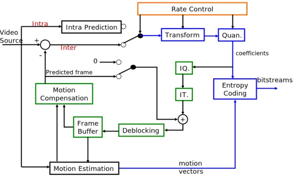
partnership known as the Joint Video Team (JVT). Fig. 2.1 shows the encoder of

Intra Prediction Motion Estimation Transform Quan. Rate Control Entropy Coding IQ. IT. Motion Compensation Frame Buffer Deblocking Intra Inter Video Source Predicted frame motion vectors coefficients bitstreams 0 + -+

Fig. 2-1 H.264/AVC Encoder

H.264/AVC contains a number of new features that allow it to compress video

much more effectively than older standards and to provide more flexibility for

application to wide variety network environments. There are several key features

including multiple reference frames, variable block size motion compensation to find

out accurate motion vectors, quarter pixel precision motion vectors, new transform

design features like integer 4x4 spatial block transform, in-loop deblocking filter

which helps prevent the block artifacts, entropy coding design such as context

adaptive binary arithmetic coding (CABAC) and context-adaptive variable length

coding (CAVLC) and so forth used for high compression performance compared to

previous video coding standards.

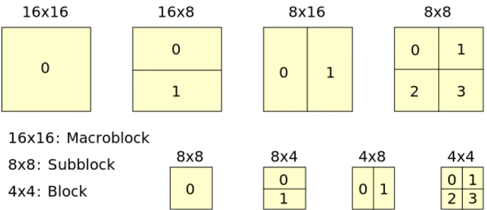
Among them, the inter mode decision process with variable block size motion

estimation part is the most complex and time consuming. The block sizes are 16x16,

16x8, 8x16, 8x8, 8x4, 4x8, and 4x4. Fig. 2.1 shows the possible macroblock modes.

Except the above seven kinds of mode, there are three more possible modes SKIP,

I4MB, and I16MB in inter frame coding. The SKIP mode is a direct copy from the

adjacent block size. In general, SKIP, 16x16, 16x8, and 8x16 are called large block

size modes, 8x8, 8x4, 4x8, and 4x4 are called small size block or sub block modes

(P8x8). 16x16 16x8 8x16 8x8 8x8 8x4 4x8 4x4 0 0 1 0 1 0 1 2 3 0 0₁ 0 1 0_{2 3}1 16x16: Macroblock 8x8: Subblock 4x4: Block

Fig. 2-2 Variable Block Size in H.264/AVC

To achieve the highest coding efficiency, the H.264/AVC reference software

encoder, JM [9], uses a non-normative technique called Lagrangian rate-distortion

optimization (RDO) technique to decide the block coding mode. Fig. 2.3 shows the

RDO process. In order to choose the best coding mode for a macroblock, H.264/AVC

encoder calculates the rate-distortion (RD) cost (RDcost) of every possible mode and

chooses the mode having the minimum value, and this process is repeatedly carried

out for all the possible modes for a given macroblock.

Encoding Transform / Quantization Variable Length Coding Inverse Transform / Inverse Quantization Compute RD cost Mode Selection Input

video Residual data

Distortion Rate

Fig. 2-3 Computation of RDcost

The best mode selected and used for coding must have the minimum cost. The

)

(

))

(

,

(

)

,

(

m

SAD

s

c

m

R

m

p

J

λ

_motion

=

+

λ

_motion

⋅

−

where is the current motion vector (MV), is the

predicted MV. represents the bits used to encode the MV information.

stands for the sum of absolute difference between current MB and

reference MB, where T y x

m

m

m

=

(

,

)

(

m

p

R

−

))

(

,

c

m

s

T y x

p

p

p

=

(

,

)

)

(

SAD

s

represents reference macroblock and stands for a function of current macroblock with a parameter motion.

)

(m

c

motion

λ

is the Lagrange multiplier, which is a function of QP,

3 / ) 12 (

2

85

.

0

)

(

=

×

QP− motion

QP

λ

From equation (1), we know that choosing a larger partition size means that

fewer bits are used to signal the MVs and other information, but the residue may

contain much higher energy, especially with more details. On the other hand, choosing

a smaller partition size may give a low residue after motion estimation but it needs to

use more bits to signal the MVs and other information. Therefore, the multiplier,

motion

λ

, can be considered as a trade-off parameter between the rate and distortion.

In this case, if encoder pays one bit to reduce more than

λ

motion distortion in SAD,

then less Lagrange cost,

J

(

m

,

λ

motion

)

, is obtained. The optimal coding efficiency

can be achieved by checking all available modes and selecting the minimum cost. To

sum up, how to select the best mode is very important to get the best performance of

the H.264 codec.

2.2 Video Transcoding

information industry. Multimedia services and applications for a network environment,

such as videoconferencing, video streaming on web application, distance e-learning,

and video on demand, are widely used recently. With video being an important part of

multimedia communications, new video compression techniques like MPEG-2,

MPEG-4 and H.26x are proposed to satisfy new applications.

Transcoding is a process of converting a previously compressed video bitstream

into a lower bit-rate video bitstream. The main function of video transcoding is that it

can provide different format conversion, resolution scaling, bit-rate conversion, and

frame rate conversion. Format conversion, for example, from MPEG-2 as input video

stream converting to H.264/AVC as output video bitstream or from MPEG-4 to

H.264/AVC, transform from original high bit-rate or low video quality format to

superior video standard, low bit-rate or high video quality video format. Bit-rate

conversion uses different quantization parameter (QP) to control the video quality and

then obtain different bit-rate. Resolution scaling makes use of the video frame

up-sizing or down-sizing to attain higher or lower bit rate. Frame rate conversion by

means of skipping some frames regularly or dynamically to reduce the frame rate but

guarantee an acceptable video quality.

In general, there are two approaches for implementing transcoding, commonly

known as pixel-domain transcoding and discrete cosine transform (DCT) domain

transcoding. The basic component of transcoding has mentioned above in Fig. 1.1. In

pixel-domain transcoding, both of the incoming video bitstream and output of the

transcoded video bitstream are decoded/re-encoded in the pixel domain. This involves

high complexity, memory, and time consuming. Discrete cosine transform (DCT)

domain transcoding which the incoming video bitstream is partially decoded to form

the DCT coefficients and downscaled by the requantization of the DCT coefficients.

t

f

the coded domain where complete decoding and re-encoding are not required. The

problem with this approach is that the quantization errors will accumulate, and a

prediction memory mismatch at the decoder will cause poor video quality called

“drift” degradation.

In this thesis, we focus on frame skipping approach in the pixel domain because

it is a good strategy for controlling the bit-rate and maintaining the picture quality

within the acceptable level. The reason is that it is difficult to perform frame skipping

in the DCT-domain since the prediction errors of each frame are computed from its

immediate past frames. This means the incoming quantized DCT coefficients of the

residual signal are no longer valid because they refer to the frames which have been

dropped.

Frame skipping transcoding for bit-rate reduction of compressed video have been

researched in many literatures [10][11]. Fig. 2.4 shows the architecture of frame

skipping transcoder. In the front encoder, the motion vector, , for a macroblock

with pixels in frame , the current frame, is computed by searching for the

best matched macroblock within a search window in the previous reconstructed

frame, , and is obtained as follows:

t

mv

N

N

×

1 − t

R

S

DCT Q1 IQ1 IDCT MC FB IQ1 IDCT FB MC DCT Q2 IQ2 IDCT MC FB (u,v) (u’,v’) IQ2 IDCT f FB MC (u’,v’) + + + + + + + + +

Front Encoder Transcoder End DecoderReceiver

)

,

(

min

arg

)

,

(

) , (

SAD

m

n

v

u

mv

S n m t t t

=

=

_∈

∑∑

− = − = −

+

+

−

=

1 0 1 0 1

(

,

)

)

,

(

)

,

(

N i N j t t

i

j

R

i

m

j

n

f

n

m

SAD

where m and n are the horizontal and vertical components of the displacement of a

matching macroblock, and represents a pixel in and ,

respectively.

) , ( ji

f_t

R

_t−1

(

i

,

j

)

f

_t R_t−1

2.3 Motion Vector Composition

In the transcoder, the optimized motion vectors (MVs) for the outgoing video

stream can be obtained by applying the full-scale full-search motion estimation.

However, the full-scale motion estimation for the Transcoder requires a high

computational complexity. Besides, in frame skipping transcoding, some incoming

frames are dropped, and the incoming motion vectors (MVs) are not valid because

they point to the dropped frames that do not exist. Generally, motion estimation has

not been computed again because of this high computational complexity. Furthermore,

using the extracted MVs from the incoming video stream for the outgoing video

stream would be almost as good as re-calculating the new motion estimation. The

re-use of MVs extracted from an incoming video bitstream during transcoding has

been widely adopted.

To find the MV for a macroblock in the current frame, a best matching

macroblock is searched within a predefined search window in the previous

reconstructed reference frame, as shown in Fig. 2.5. The MV is defined as the

motion estimation is performed on the luminance macroblocks and is usually based on

the sum of absolute differences (SAD) of the pixels in current video coding standards.

Previous reference frame Current frame Search window

Motion vector

Best match block

R (x, y) P (x, y)

Fig. 2-5 Block Matching Motion Estimation Algorithm

Re-use of incoming motion vector can be achieved by bilinear interpolation and

forward dominant vector selection (FDVS) [7]. In [12], bilinear interpolation is

defined as: 2 1

(

1

)

)

1

)(

1

(

MV

MV

MV

_BI

= −

α

−

β

+

α

−

β

4 3

)

1

(

α

MV

αβ

MV

β

−

+

+

where , , , and are the motion vectors of the four

macroblocks overlapping the reference area in the skipped frame pointed by the

incoming motion vector. 1

MV

MV

₂

MV

₃

MV

₄

α

and

β

are determined by the horizontal and vertical pixel distance of this reference area from . Fig. 2.6 illustrates the interpolation

of the motion vector.

1

MV

α

MV₁ MV₃ MV₂ MV₄ β Motion estimated MB

Fig. 2-6 Interpolation of Motion Vectors

skipped, is Motion Vector Composition (MVC) shown in Fig. 2.7. The goal of motion

vector composition scheme is to find a motion vector in the last skipped frame, to be

composed with the motion vector of the current frame, in order to obtain a motion

vector for the current frame that points to the last skipped frame. The advantage of

MVC is that, it is very easy to compute a motion vector for such macroblocks, given

that their reference area exactly overlaps a macroblock in the skipped frame.

F(n-2) F(n-1) F(n)

skipped

MVC

Fig. 2-7 Motion Vector Composition

Forward dominant vector selection (FDVS) [7] is used for composing the target

MV from the four MVs of the four neighboring macroblocks. Combine with the

concept of MVC mentioned above, as Fig. 2.8 shows, we assume that MV2 and MV3

represent the MV for the block in frame (n-1) and frame (n-2), respectively. Since

frame (n-1) is dropped, we need to find a MB pointing to a block in frame (n-2). A

feasible solution to generate a MV without performing motion estimation is to use the

vector sum of MV. However, there is no block on macroblock boundary actually.

Hence, MV2 is not available from the incoming video bitstream. The approach of

FDVS selects one dominant MV from the four neighboring macroblocks. A dominant

MV is defined as the MV carried by a dominant macroblock and the dominant

macroblock is a macroblock that has the largest overlapping area with the block

I₁n-3 _I 2n-3 I₃n-3 _I 4n-3 I₁n-2 _I 2n-2 I₃n-2 _I 4n-2 I₁n-1 _I 2n-1 I₃n-1 _I 4n-1 I₁n _I 2n I₃n _I 4n MV₁ MV₂ MV₃ MVC 16 16 dropped dropped

Frame (n-3) Frame (n-2) Frame (n-1) Frame (n)

Fig. 2-8 Backward MV Composition: MVC = MV1+MV2+MV3

16 MV dropped dropped 1 MV₂ MV₃ 16

Frame (n-3) Frame (n-2) Frame (n-1) Frame (n)

Fig. 2-9 FDVS Composition Scheme

The FDVS gets much better performance than the bilinear interpolation scheme,

and the bilinear interpolation for composition for MVs is with high computation.

Next, we introduce another algorithm that it also decides the dominant MV from

four neighboring macroblocks called activity dominant vector selection (ADVS) [6].

The conception of ADVS is the decided MV should be toward the MV with the larger

prediction error. To gain a measure of the prediction error directly from the existing

compressed bitstream, the DCT energy in the residual blocks is measured. ADVS

algorithm utilizes the activity of the macroblock to decide the choice of the MV. Here,

the activity information of a macroblock is represented by counting the number of

quantities are proportional to the spatial-activity measurement. As shown in Fig. 2-10,

the MV of the macroblock with the maximum NZ (number of nonzero quantized DCT

coefficients) is selected by the ADVS scheme as the dominant MV.

I₁₁n-1_I 12n-1I21n-1I22n-1 I₁₃n-1_I14n-1_I 23n-1I24n-1 I₃₁n-1_I 32n-1I41n-1I42n-1 I₃₃n-1_I 34n-1I43n-1I44n-1 NZ (I₁n-1_{) NZ (I} 2n-1) NZ (I₃n-1_{) NZ (I} 4n-1) 16 16 8 8

Fig. 2-10 Illustration of the ADVS Algorithm

where

NZ

(

I

₁n−1

)

=

NZ

(

I

₁₂n−1

)

+

NZ

(

I

₁₄n−1

)

)

(

)

(

)

(

)

(

)

(

I

₂n−1

=

NZ

I

₂₁n−1

+

NZ

I

₂₂n−1

+

NZ

I

₂₃n−1

+

NZ

I

₂₄n−1

NZ

42 41 4 )) ( ) (I₃n−1 =NZ I₃₂n−1 NZ ) ( ) ( ) (I n−1 = NZ I n−1 +NZ I n−1 NZ : (.)

NZ number of nonzero quantized DCT coefficients

The bigger the activity (NZ) of the macroblock, the more significant the motion of the

macroblock. Sine the quantized DCT coefficients of prediction errors are available in

the incoming stream of transcoder, the computation for counting the nonzero

Chapter 3 The Propose Method

In this chapter, we describe the proposed frame skipping transcoding algorithm

in detail. Section 3.1 includes the overall system architecture and the flowchart of the

proposed method. Section 3.2 focuses on how to select block mode type. Section 3.3

contains not only applying the original approaches like FDVS, ADVS, and PADVS(n)

to several macroblock types in H.264/AVC video frame skipping transcoding, but also

introducing our proposed algorithm suitable for all block mode types in H.264/AVC.

3.1 System Architecture

Figure 3.1 shows our H.264/AVC video frame skipping transcoding architecture.

The transcoding architecture includes a full H.264/AVC decoder and a H.264/AVC

transcoding encoder. Comparing Figure 2.4 to Figure 3.1, both the segments of the red

dotted line show the most important part in our transcoding architecture.

H.264 Decoder MV info. MB mode Coeff. H.264 video stream incoming stream Proposed MV Decision Proposed

Mode Decision _modeMB M.E. Transform

Quan. Entropy Coding outgoing stream H.264 video stream Transcoding

Fig. 3-1 Proposed H.264/AVC video frame Skipping Transcoding Architecture

Both of input and output streams are H.264/AVC standard format, the main

operating units of transcoding architecture according to the chapter 1. We divide them

back-end decoder which have been shown in figure 1.1. Among them, front-end

decoder and back-end encoder are the focus of this thesis so they are depicted in

figure 3.1, where both the incoming stream and outgoing stream are in H.264/AVC

format.

In this architecture, when the H.264/AVC video stream has been decoded, we

would save some information including motion vectors, macroblock types, and

residual coefficients from the compressed video stream. And then in the H.264/AVC

transcoding part, we concentrate on mode decision and motion vector decision parts.

Other parts follow the standard H.264/AVC encoding procedures to produce the

stream. The propose mode decision uses the macroblock types and residual

coefficients obtained from incoming H.264/AVC compressed video stream while the

propose motion vector decision uses the motion vectors and macroblock types. Both

of the propose methods reuse the information from incoming video stream, so that we

can save a lot of time cost and computational complexity in doing motion estimation

and rate-distortion optimization, both of which take a great majority of time

consuming in the transcoding process.

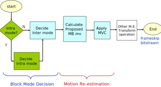
Figure 3.2 shows the flowchart of the proposed block mode decision and motion

vector decision methods. The first stage performs block mode decision which makes

the decision of the block mode. The second stage of the flowchart is to do the motion

start intra mode? Decide intra mode Decide inter mode Calculate Proposed MB mv Apply MVC frameskip bitstream N Y Other M.E. Transform operation End Motion Re-estimation Block Mode Decision

Fig. 3-2 Flowchart of Proposed Block Mode and MV Decision Methods

3.2 Proposed Block Mode Decision Method

In H.264/AVC video coding standard, it employs several different macroblock

mode types in intra and inter blocks. They are I16MB and I4MB in intra macroblocks,

and PSKIP, P16x16, P16x8, P8x16, SMB8x8, SMB8x4, SMB4x8 and SMB4x4 in

inter macroblocks, respectively. H.264/AVC standard software, JM, uses Lagrangian

rate-distortion optimization (RDO) technique to decide the block coding mode and

motion vector. However, the computation complexity of calculating Lagrangian

function for every block is quite high. Therefore, a fast block mode decision to

determine block mode is important.

Figure 3.3 shows the flowchart of the proposed block mode decision method,

where the input is a video stream including skipped frames and non-skipped frames.

The next paragraph would show how to do the block mode decision.

Let denote the current frame, and denote the corresponding

reference frame which will be dropped. The following steps are performed to

determine the mode for each macroblock in .

cur

f

f

_skip

cur

f

i cur

MB

the macroblocks as and , respectively. If anyone of and

is intra mode then intra mode is selected and rate-distortion optimization is

applied on to decide whether intra4x4 or intra16x16 to be used. However, if

none of and is intra mode, the mode-change rules in Table 3.1 are

applied to obtain a candidate block mode for . All these mode-change rules

follow the principle that the smaller block mode between and is

selected as the candidate mode. It is due to the fact that, after has beed

dropped, the sidtance between and its new reference frame increases, and

therefore, smaller block mode should be more suitable.

i skip

MB

cur

MB

i cur

MB

cur i skip

MB

cur

MB

skip i cur

MB

i cur

MB

i skip

MB

i i skip

MB

i

f

f

In final step of the flowchart, we sub-divided the inter block with candidate

block mode into more blocks with smaller block modes in order to gain better visual

quality and lower rate-distortion cost. Figure 3.3 presentd four macroblocks as

examples. For the left-top macroblock, the candidate block mode resulting from mode

change step is P8x16 and will be sub-divided into SMB8x8 for rate-distortion cost

(RDcost) evaluation. If the resulting four 8x8 blocks get a better RDcost than the two

P8x16 blocks, the sub-division process repeat; otherwise, the block mode of P8x16 is

selected. For the left-down macroblock, the block P16x16 could be sub-divided into

two P8x16 blocks, or two P16x8 blocks as shown in the right side of the two arrows.

For each sub-division case, the RDcost is calculated, if it is smaller than the one

RDcost of the one without division, then we should adopt the divided one and the

dividing process repeat again. Otherwise, we stop dividing the inter block.

Divide inter block Divide inter block Mode change result

check 1

check 2

Fig. 3-3 Divide Inter Block

Rule 1 Select intra mode if it exists among co-located macroblock in the either current frame or previous frame

Rule 2 Select the smaller mode type between skipped and non-skipped frames Rule 2.1 Choose P16x16 if one of them is P16x16 or PSKIP and the

other is P16x16

Rule 2.2 Choose P16x8 if one of them is P16x16, P16x8, or PSKIP and the other is P16x8

Rule 2.3 Choose P8x16 if one of them is P16x16, P8x16, or PSKIP and the other is P8x16

Rule 2.4 Choose SMB8x8 if one of them is P16x16, P16x8, P8x16, PSKIP, or SMB8x8 and the other is SMB8x8

Rule 2.5 Choose SMB8x4 if one of them is P16x16, P16x8, P8x16, SMB8x8, or SMB8x4 and the other is SMB8x4

Rule 2.6 Choose SMB4x8 if one of them is P16x16, P16x8, P8x16, SMB8x8, or SMB4x8 and the other is SMB4x8

Rule 2.7 Choose SMB4x4 if one of them is P16x16, P16x8, P8x16, SMB8x8, SMB8x4, SMB4x8, or SMB4x4 and the other is SMB4x4

Rule 3 Special Case

Select SMB8x8 if one of them is P16x8 and the other is P8x16 Select SMB4x4 if one of them is SMB8x4 and the other is SMB4x8

Rule 4 Select SKIP mode only if both of skipped and non-skipped are SKIP modes

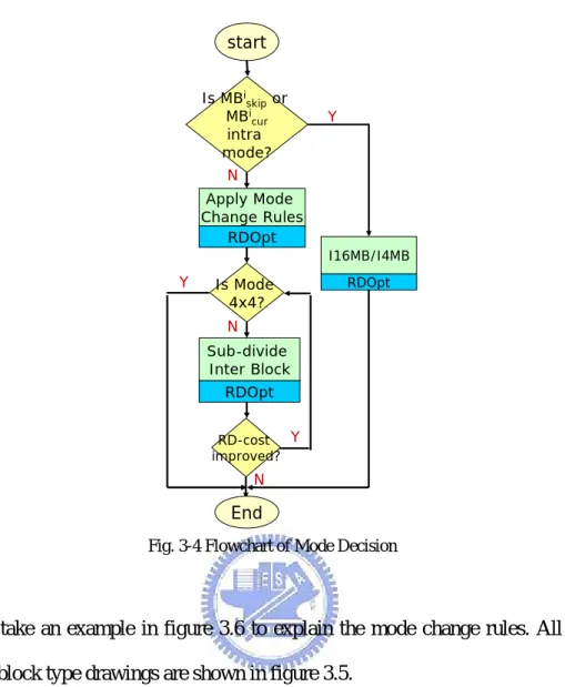
Is MBi skipor MBi cur intra mode? Y Apply Mode Change Rules N RD-cost improved? Sub-divide Inter Block N RDOpt Y I16MB/I4MB RDOpt start End RDOpt Is Mode 4x4? Y N

Fig. 3-4 Flowchart of Mode Decision

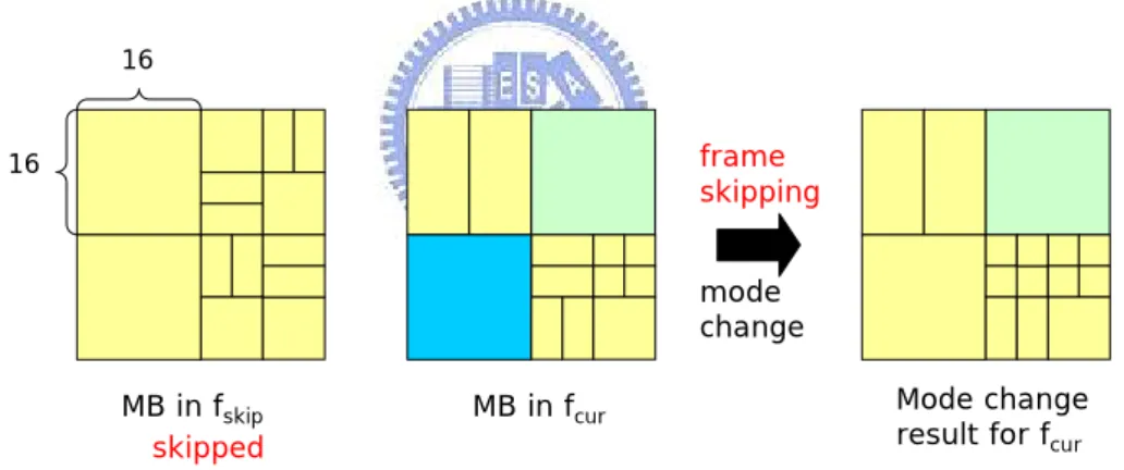
We take an example in figure 3.6 to explain the mode change rules. All of the

variable block type drawings are shown in figure 3.5.

P16x16 P16x8 P8x16 SMB8x8

SMB8x4 SMB4x8 SMB4x4 I16MB I4MB

PSKIP

Fig. 3-5 Variable Block Mode

In figure 3.6, is the current frame for mode decision and is the

corresponding reference frame that will be skipped after transcoding. To simplify the

illustration, each frame consists of four macroblocks.

cur

The block mode of upper-left macroblock is P16x16 in and P8x16 in

. Therefore, after applying mode change rule 2.2, the resulting block mode for

should be P8x16. As for block mode decision of upper-right and lower-left

macroblocks, the resulting modes should be intra16x16 and P16x16, respectively, due

to rule 1 and rule 2.1. The final part of the example is more complicated and it

contains four sub-macroblocks. The upper-left sub-macroblock is SMB4x8 in

and SMB8x4 in , so after applying rule 3, the resulting block mode should be

SMB4x4. Similar processes are performed for all the other three sub-macroblocks,

and the resulting sub-block modes are shown in the right hand side of figure 3.6.

skip

f

cur

f

skip

f

skip

f

cur

f

16 16 MB in f_skip MB in f_cur frame skipping mode change Mode change result for f_cur skipped

Fig. 3-6 Mode Change Result

3.3 Proposed Motion Vector Composition Method

Motion estimation is also an important segment in video frame skipping

transcoding. In this section, we discuss about how to employ the motion re-estimation

by using the motion vectors obtained from front-end transcoder. An enhanced FDVS

3.3.1 Enhanced FDVS Method for H.264/AVC

The enhanced FDVS method mentioned in this section is suitable for all kinds of

mode including variable block size of inter, intra, and SKIP mode. Owing to the

fundamental conception of implementing FDVS method is to find out macroblcok

that has the largest area overlapped with the area pointed by the motion vector of

current macroblock as dominant macroblock, and then use the motion vector of the

dominant macroblock as dominant motion vector. However, there exist two problems

if we directly apply the FDVS idea to H.264/AVC video coding. Firstly, finding the

largest overlapping area in the variable block size in H.264/AVC is much complicated

due to the quarter-pixel precision and complex combinations of various block modes.

Secondly, the dominant macroblock may be the smallest block size such as SMB4x4.

Therefore, in some cases, the results of motion vector selected by original FDVS and

by enhanced FDVS method may be different. The reasons will be explained in this

section by examples.

For above reasons, we suggest another flexible manner to prevent from the

foregoing conditions. We divide all inter block modes into different numbers of inter

4x4 FDVS unit, as shown in figure 3.7. For instances, a P16x16, P16x8, SMB8x8,

and SMB4x4 blocks would be divided into sixteen, eight, four, and one 4x4 FDVS

units, respectively.

4 4 current mv

Fig. 3-7 An Inter 4x4 FDVS Unit

The center of each FDVS unit can be found out. The center position is marked as

each 4x4 FDVS unit, we add up center location and current motion vector. The

motion vector of macroblock which is pointed to is one of the candidate motion

vectors. The program takes down all candidate motion vectors, and looks for the

motion vector appearing most frequently as the dominant motion vector. Take an

example, suppose four candidate motion vector of a SMB8x8 macroblock are (1, 0),

(0, 1), (2, 0), and (1, 0). The candidate motion vector of (1, 0) appears twice so that it

becomes the most frequent candidate motion vector. And then (1, 0) would be the

dominant motion vector of the SMB8x8 macroblock. The results of using center point

methods can save a lot of time without calculating the overlapped area.

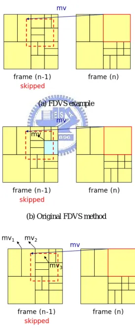
Take an example in figure 3.8 to explain the difference between original FDVS

method and enhanced FDVS method. We focus on the upper-right part of P16x16

macroblock in frame (n). Figure 3.8 describes that after adding the current motion

vector, P16x16 refers to the red dotted line in the frame (n-1). The macroblock type

under the red dotted line contains a P8x16, a P16x16, two SMB8x8, two SMB8x4,

and four SMB4x8. If we choose the original FDVS method, we have to pick up the

largest overlapped area referenced in the frame (n-1). For an instance, suppose the

largest overlapped area is SMB8x8 located at the lower-right partition, as figure 3.8 (b)

shows. The blue area of SMB8x8 block is selected by original FDVS method which it

contains the largest partition. In our propose method, enhanced FDVS method, we not

only check all the center points that current macroblock refers to, but also accumulate

the same length of motion vectors. As figure 3.8 (c) shows, assume that the length of

three motion vectors , , and are (2, 1), (2,1), and (1,1). If the

macroblocks of and contain two 4x4 FDVS units while the macroblock

of contains three 4x4 FDVS units. However, the length of and is

the same so that we accumulate the same length of motion vector even if they belong 1

mv

mv

₂ 2

mv

3

mv

1

mv

3

mv

mv

₁

mv

₂

to different macroblocks.

Hence, we select as dominant motion vector if we use original FDVS

method, while we will choose or as dominant motion vector if we use

our propose enhanced FDVS method. The main difference between original FDVS

and enhanced FDVS is that our propose method selects the motion vector which

appears most frequently. 3

mv

1

mv

mv

₂ mv frame (n-1) frame (n) skipped (a) FDVS example mv frame (n-1) mv frame (n) skipped (b) Original FDVS method frame (n-1) skipped frame (n) mv mv1 mv2 mv3 (c) Enhanced FDVS method

Fig. 3-8 (a) FDVS example (b) Original FDVS method (c) Enhanced FDVS method

macroblock, the dominant motion vector selected by the proposed enhanced FDVS is

different from that selected by original FDVS. Now assume the mode change step

determines to use 8x8 block mode (instead of 16x16) for current macroblock.

As the figure 3.9 shows, P16x16 macroblock should be divided according to the

block mode decision. Each 8x8 block then is sub-divided into 4x4 FDVS units which

are mapping to the reference frame (n-1). On frame (n-1) it shows that the upper-left

SMB8x8 is overlapped with a 8x16 bocks with , a 8x8 block with , and a

8x4 block with , respectively. Since there are two central points of FDVS units

located in the block with , and only one in and , the dominant

motion vector is set to .

1

mv

mv

₂ 3

mv

1

mv

1 2

mv

mv

₃

mv

mv Mode Decision mv₁ mv₂ frame (n-1) P16x16 mv₃ 16 16 skipped

Fig. 3-9 Enhanced FDVS Example Result

3.3.2 Enhanced ADVS Method for H.264/AVC

Another proposed method, enhanced ADVS, is derived from the conception of

ADVS is to accumulate each non-zero quantized coefficients of block covered in.

Unlike the way applying ADVS to all 16x16 modes, applying ADVS to all kinds of

block modes produce some different issues. As figure 3.10 shows an 4x4 inter ADVS

unit. Other kinds of macroblock types are based on the 4x4 inter ADVS unit and

divided into several ADVS units. As we can see in figure 3.11 illustrates SMB8x4,

SMB4x8, and SMB8x8 block type divided into ADVS units.

4 4 current mv

Fig. 3-10 An 4x4 Inter ADVS Unit

We propose to check the endpoints of ADVS unit point to the location after

adding the current motion vector. The endpoints are labeled as small blue circles as in

the figure 3.10 and 3.11. Each 4x4 inter ADVS unit would have four endpoints.

Similarly, there are six endpoints in a SMBx4 or SMB4x8 block, nine endpoints in a

SMB8x8 block, fifteen endpoints in a P16x8 or P8x16 block, and twenty-five

endpoints in a P16x16 block. current mv 8 4 8 4 current mv 8 8 current mv

Fig. 3-11 SMB8x4, SMB4x8, SMB8x8 Check Endpoint

As figure 3.12 shows, we explain the overall process by an example. Suppose

current macroblock is a P16x16 block mode. After applying mode decision as before,

and map them to the previous frame (n-1). For the left-top SMB8x8 block, there are

three endpoints locating at the P8x16 with in the previous frame (n-1) we have

to calculate its non-zero quantized coefficients. Four endpoints are located at the

SMB8x8 with in the previous frame and we have to count its non-zero

quantized coefficients. The remaining two endpoints are located at the SMB8x4 we

also calculate its nonzero quantized coefficients. By comparing the NZ(.) results of

three different groups, presume that the one with maximum of non-zero quantized

coefficients is the block SMB8x8 with , then we would consider the motion

vector as our dominant motion vector. 1

mv

2

mv

2

mv

2

mv

mv Mode Decision mv₁ mv₂ frame (n-1) P16x16 mv₃ 4x4 NZ unit skipped

Fig. 3-12 Apply ADVS Example

3.4 MV Selections for Mode Change and No Mode Change

In this section, we probe the effectiveness of the mode change. For comparison,

figure 3.13 (a) illustrates the case with mode change, while figure 3.13 (b) shows the

and the co-located macroblock in the reference frame (n-1) is composed of four

SMB8x8. After doing the proposed mode change method as well as enhanced FDVS

or enhanced ADVS, the outcome would be four SMB8x8 block modes with different

motion vectors. Oppositely, if we have the same block mode without using mode

change, we would retain the block mode of non-skipped frame with a determined

motion vector as illustrated in the figure 3.13 (b).

frame (n-1) frame (n) skipped mv mode change frame (n/2) frame skipping mv₁ mv₂ mv_{3 mv} 4

(a) mode change

frame (n-1)

’

skipped frame (n) mv mv frame skipping frame (n/2) (b) no mode change

Fig. 3-13 MV selections for (a) mode change and (b) no mode change

The experimental results of the mode change and no mode change will exhibit in

the chapter 4.

3.5 Apply Motion Vector Composition

No matter enhanced FDVS or enhanced ADVS is adopt to obtain the dominant

The typical strategy we use for motion vectors computation when a frame is skipped,

is called motion vector composition (MVC) shown in figure 3.14. The goal of motion

vector composition scheme is to compose the dominant motion vector in the

skipped frame with the motion vector of the current frame in order to obtain a motion

vector for the current frame that points to the previous non-skipped frame which is

used as the new reference frame.

MVC current mv by propose method Dominant mv: F(n-2) F(n-1) F(n) skipped

Fig. 3-14 Apply Motion Vector Composition

The benefit of MVC is that, to compute a motion vector for such

macroblock is simpler because it effectively reuses the information from the encoded

Chapter 4 Experimental Results

In this chapter, we compare the proposed methods with the general FDVS [7],

ADVS [6], and PADVS [8] algorithms, which speed up the motion vector

composition, respectively. We also compare the proposed transcoder with the optimal

frame skipping method proposed in H.264/AVC JM13.2 reference software. Various

types of standard test sequences with CIF (352x288) format are tested.

The proposed transcoder is implemented by using the H.264/AVC JM13.2

reference software. The parameters of our experimental environments are set as

following:

Hardware Parameters:

CPU: Intel Pentium Core 2 Due 1.83GHz, 1.83GHz

RAM: 2.00 GB

Software Parameters:

Test sequences: Foreman, Football, Tennis, Stefan, bus, Container, Hall

Frame Format: CIF (352x288 pixels)

Group of Picture (GOP): I P P P P …, and the period of I-frame is 30.

Frame Rate: 30 fps

Number of reference frame: 1

Motion Estimation: Search window size = 32, fast full search

R-D Optimization: High complexity mode

Inter Mode: All mode are enabled

Intra Mode: I16MB and I4MB enabled

We conducted experiments of different methods in this section. First, we applied

which only use P16x16, PSKIP, and I16MB macroblock type. The reason is that all of

three methods are used in MPEG-2 video coding standard originally.

Second, we separate our proposed method, mode decision and motion vector

composition, into two cases. One is with motion vector composition with mode

decision and the other is without mode decision. The destination is to observe the

influence on mode decision.

Finally, we would compare our proposed method with JM 13.2 reference

software, FDVS, ADVS, and PADVS(n).

4.1 FDVS, ADVS, and PADVS(n) Methods on Large Block Sizes

Several sequences tested in this section would show that the methods of FDVS,

ADVS, and PADVS(n) save a lot of time of transcoding and motion estimation with

acceptable degradation of video quality and slightly increase in bit-rate. The definition

of large block size is block type of P16x16, PSKIP, and intra16x16MB. The test

sequences are foreman, news, hall, football, and flower, where news and hall are

classified as slow or smooth motion sequences, foreman and flower are median

motion, and football is high motion. The parameter n in the PADVS(n) method is

established as n=1, 3, 10, 36, and 49 that covered, where the non-zero quantized

coefficients are selected in a zig-zag scan order from low frequency to high frequency.

The numbers of frame sequences before and after frame skipping transcoding are 120

and 60, respectively. For the sequence, one frame is skipped for every two frames.

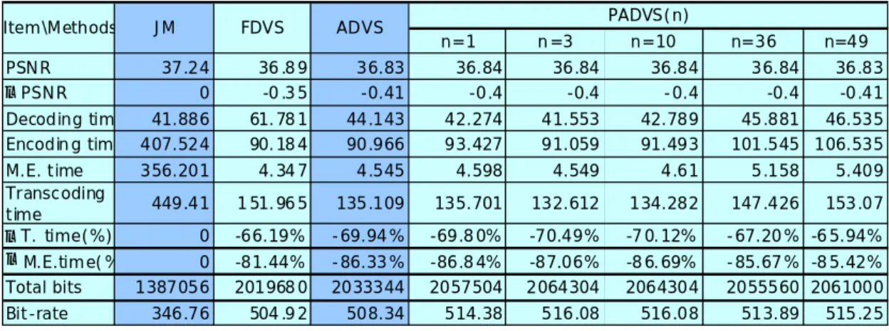
Table 4.1 describes the results of JM, FDVS, ADVS, and PADVS(n) methods

applying to “foreman” on large block size. The experimental results show that

comparing to reference software JM, the methods of FDVS, ADVS, and PADVS(n)

decrease 0.35dB to 0.41dB in PSNR measurement while saving about 65% to 70% in

n=1 n =3 n=10 n=36 n=49 PSNR 37.24 36 .8 9 36.83 36.84 36.84 36.84 36.84 36.83 △PSNR 0 -0 .3 5 -0.41 -0.4 -0.4 -0.4 -0.4 -0. Decoding tim 41.886 61.78 1 44.143 42.274 41.553 42.789 45.881 46.535 Encodin g tim 407.524 90.18 4 90.966 93.427 91.059 91.493 101.545 106.535 M.E. time 356.201 4.34 7 4.545 4.598 4.549 4.61 5.158 5.409 Transcoding time 449.41 1 51.96 5 135.109 135.701 132.612 134.282 147.426 153.07 △T. time(%) 0 -66.19% -69.94% -69.8 0% -70.49% -7 0.12% -67.20% -6 5.94% △M.E.time( 41 % 0 -81.44% -86.33% -86.8 4% -87.06% -8 6.69% -85.67% -8 5.42% Total bits 1387056 201968 0 2033344 2057504 2064304 2064304 2055560 2061000 Bit-rate 346.76 504 .9 2 508.34 514.38 516.08 516.08 513.89 515.25 PADVS(n) FDVS ADVS Item\Methods JM

Table 4-1 Experimental results of FDVS, ADVS and PADVS(n) on foreman.cif

Here we define some terms such as

Δ

PSNR

,

Δ

T .

time

, and as followings:

time

E

M

.

.

Δ

JM PSNR method PSNR PSNR =Δ _ −Δ _ Δ

△ PSNR means the degradation of PSNR compared with the full H.264/AVC

re-encoder.

time

T .

Δ

: stands for the percentage of reduced processing time comparing with the H.264/AVC re-encoder. The formula is listed as below:

JM Time JM Time method Time time Total _ =( _ _ )/ _ Δ −

time

E

M

.

.

Δ

: stands for the percentage of reduced motion estimation time comparing with the H.264/AVC re-encoder. M.E. is the abbreviation of motion

estimation. JM E M JM E M method E M time E M. . =( . _ − . ._ )/ . ._ Δ

where the “method” in above formula could be FDVS, ADVS, or PADVS (n). Notice

that the definition of transcoding time is the summation of decoding time and

encoding time. From Table 4.1, the experimental results show that the visual quality

of FDVS, ADVS, and PADVS(n) are close to JM in PSNR measurement. However,

due to only using large block size, some proportions of macroblocks are encoded as

Therefore, the bit-rates increase when using FDVS, ADVS, and PADVS(n) methods.

The phenomenon can be solved if we use all block modes to encode the macroblocks.

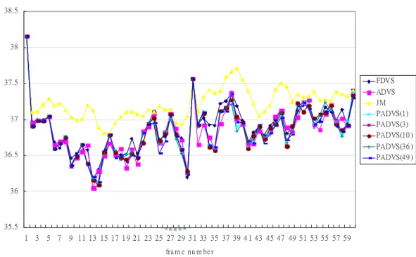
Figure 4.1 shows the PSNR measurement frame by frame in foreman sequence.

The yellow curve is the result of conducting by JM while the blue and pink curves are

representation of FDVS and ADVS.

35.5 36 36.5 37 37.5 38 38.5 1 3 5 7 9 11 13 15 17 1 9 21 23 25 27 29 3 1 33 35 37 39 4 1 43 45 47 49 51 53 55 57 59 fra m e nu m be r PS N R FDVS ADVS JM PADVS(1) PADVS(3) PADVS(10 ) PADVS(36 ) PADVS(49 )

Fig. 4-1 Different Methods in PSNR Frame by Frame in Foreman

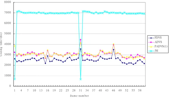
Figure 4.2 illustrates the comparison in encoding time and transcoding time in

the same test sequence frame by frame. The definition of transcoding here means the

0 1 0 0 0 2 0 0 0 3 0 0 0 4 0 0 0 5 0 0 0 6 0 0 0 7 0 0 0 8 0 0 0 1 4 7 1 0 1 3 1 6 1 9 2 2 2 5 2 8 3 1 3 4 3 7 4 0 4 3 4 6 4 9 5 2 5 5 5 8 fra m e n u m b e r Co d in g T im e ( m s) FDVS ADVS PADVS(1 ) JM

Fig. 4-2 Comparison Encoding Time with Transcoding Time Frame by Frame in Foreman

In figure 4.2, the intra periodic is set up as 30. Therefore, JM does not have to

decide the macroblock is intra or inter when encoding each I-frame. The encoding

time displays a period of declination every thirty frames. In our frame skipping

transcoding methods, we do not consider about I-frame or P-frame from the video

source but performing the mode change and motion re-estimation every two frames.

Hence, the transcoding time rises every fifteen frames.

The sequence, foreman, represents the case of median to high motion one. In

Appendix C, we will take other experimental sequences such as “news”, “hall”,

“football”, and “flower” to show our experimental results.

4.2 Propose Methods on All Block Sizes

In this section, we use the same video test sequences as input mentioned in the

section 4.3.1. Here, we focus on the experimental results of enhanced FDVS and

apply ADVS on all block size that the methods including block mode decision and

motion vector decision we proposed in the chapter 3. The term, all block sizes, means

SMB4x4, Intra16MB, and Intra4x4MB.

Table 4.2 to Table 4.4 illustrates the propose methods comparing to the reference

software JM. The term, transcoding time stands for the summation of the decoding

time and encoding time. The formulas of other terms are listed above in the section

4.3.1. PSNR 37.37 37.28 37.24 △PSNR 0 -0.09 -0.13 Decoding tim 40.612 46.593 56.251 Encoding tim 667.942 287.41 287.41 M.E. time 466.319 167.27 171.3 Transcoding time 708.554 334.003 343.661 △T. time(%) 0 -52.86% -51.50% △M.E.time(% 0 -64.13% -63.27% Total bits 1110216 1122888 1145720 Bit-rate 277.55 280.72 286.43 E-FDVS E-ADVS JM Item\Methods

Table 4-2 Propose Methods Comparing to H.264 (foreman)

PSNR 38.77 38.49 38.44 △PSNR 0 -0.28 -0.33 Decoding tim 35.88 39.36 42.28 Encoding tim 638.815 257.471 262.821 M.E. time 450.187 131.57 134.301 Transcoding time 674.695 296.831 305.101 △T. time(%) 0 -56.01% -54.78% △_{M.E.time(% 0 -62.03% -60.78%} Total bits 715416 912328 925120 Bit-rate 178.25 228.08 231.28 E-FDVS E-ADVS Item\Methods JM

Table 4-3 Propose Methods Comparing to H.264 (news)

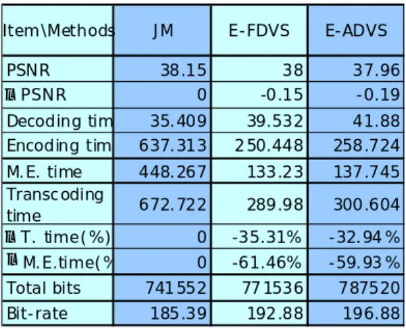
PSNR 38.15 38 37.96 △PSNR 0 -0.15 -0.19 Decoding tim 35.409 39.532 41.88 Encoding tim 637.313 250.448 258.724 M.E. time 448.267 133.23 137.745 Transcoding time 672.722 289.98 300.604 △T. time(%) 0 -35.31% -32.94% △M.E.time(% 0 -61.46% -59.93% Total bits 741552 77 1536 787520 Bit-rate 185.39 192.88 196.88

Item\Methods JM E-FDVS E-ADVS

Table 4-4 Propose Methods Comparing to H.264 (hall)

method only decreases 0.09dB to 0.28dB in PSNR measurement while saving around

35% to 56% in total time and 61% to 64% in motion estimation time. Enhanced

ADVS method decreases 0.19dB to 0.33dB in PSNR measurement while saving about

33% to 54% in total time and 60% to 63% in motion estimation time. The results

improve 0.15dB and 0.2dB comparing to large block size when using FDVS and

ADVS methods mentioned in the section 4.3.1. Table 4.5 shows the results of

comparing to the terms in bit-rate.

method\Item PSNR Total bits Bit-rate

JM 37.37 1110216 277.55 E-FDVS 37.28 1122888 280.72 E-ADVS 37.24 1145720 286.43 JM 38.77 715416 178.25 E-FDVS 38.49 912328 228.08 E-ADVS 38.44 925120 231.28 JM 38.15 741552 185.39 E-FDVS 38.00 771536 192.88 E-ADVS 37.96 787520 196.88 JM 35.32 4910904 1227.73 E-FDVS 35.26 6259720 1564.23 E-ADVS 35.18 6240010 1560.42 foreman news hall football

Table 4-5 Bit-rate of Propose Methods Comparing to H.264

Both of our propose methods, enhanced FDVS and enhanced ADVS, save a lot

of bit-rate. This is because our propose methods do the operating of mode change and

sub-division inter block to check whether the block need to be divided or not in aspect

of RDcost. When we select the smaller inter block instead of choosing intra block, we

have larger chance to save more bit-rate.

Figure 4.3 to figure 4.5 illustrate the bit-rate of different methods including JM

on all modes, E-FDVS, E-ADVS, JM on large block size, FDVS, and ADVS in

“foreman”, “news”, and “hall”. The figure shows that our propose methods are close

0 1 00 2 00 3 00 4 00 5 00 6 00 JM E-FDVS E- AD VS JM o n 1 6x1 6 FD VS o n 16 x16 ADVS o n 1 6x1 6 M et h o d s Bi t-ra te

Fig. 4-3 Bit-rate of Different Methods in Foreman

0 50 100 150 200 250 300 JM E- FD VS E-ADVS JM on 1 6x16 FDVS on 16 x1 6 ADVS on 1 6x1 6 M et ho d s Bi t-ra te

Fig. 4-4 Bit-rate of Different Methods in News

0 1 00 2 00 3 00 4 00 5 00 6 00 JM E- FDVS E-ADVS JM on 16x16 FDVS on 16x16 ADVS o n 1 6x16 M et h o ds Bi t-ra te

4.3 MV Selections for Mode Change and No Mode Change

In this thesis, we also curious about the effectiveness of the mode decision when

we adopt the mode change in our propose mode decision flowchart or not. The

quantity result of motion vector would change along with different block mode

outcome. The procedure of how to do mode change and no mode change has brought

up in the section 3.4.

Table 4.6 to Table 4.8 show the experimental results of mode change and no

mode change.

PSNR 37.37 37.28 37.18

△PSNR 0 -0.09 -0.19

Decod ing time 40.612 46.593 48.874 Encoding time 667.942 287.41 311.485 M.E. time 466.319 167.27 6.805 Transcoding time 708.554 334.003 360.359 △T. time(%) 0 -52.86% -49.14% △_{M.E.time(%) 0 -64.13% -98.54%} Total bits 1110216 1122888 2535128 Bit-rate 277.55 280.72 633.78

Item\Methods JM E-FDVS no mode_change

Table 4-6 Comparing Mode Change with No Mode Change in foreman

PSNR 38.77 38.49 38.37 △PSN R 0 -0.28 -0.4 Decoding time 35.88 39.36 41.504 Encoding time 638.815 257.471 272.035 M.E. time 450.187 131.57 2.108 Transcoding time 674.695 296.831 313.539 △T. time(%) 0 -56.01% -53.53% △M.E.time(%) 0 -62.03% -90.31% Total bits 715416 912328 1256216 Bit-rate 178.25 228.08 314.05

Item\Methods JM E-FDVS no mode

change

PSNR 38.15 38 37.91 △PSNR 0 -0.15 -0.24 Decoding time 35.409 39.532 42.421 Encoding time 637.313 250.448 265.067 M.E. time 448.267 133.23 4.089 Transcoding time 672.722 289.98 307.488 △T. time(%) 0 -35.31% -31.41% △M.E.time(%) 0 -61.46% -89.62% Total bits 741552 771536 985032 Bit-rate 185.39 192.88 246.26 E-FDVS

Item\Methods JM no mode_chage

Table 4-8 Comparing Mode Change with No Mode Change in hall

Although the method of no mode change saves more time, it also increases the

bit-rate. The experimental results show that the effectiveness of mode change

improves 0.09dB to 0.12dB in PSNR measurement when comparing to no mode

change. Therefore, it is worthy of operating mode change to reduce bit-rate and

Chapter 5 Conclusion

An efficient frame skipping transcoding from H.264/AVC to H.264/AVC

including mode decision and motion vector decision methods had been proposed. In

our propose methods, we obtain some information from the compressed video stream

in H.264/AVC and then reuse them to decide the block mode types and motion

vectors in the retained frame.

Our propose methods save more than 50% transcoding time and visual quality

only reduced less than 0.2dB in most of the test sequences when comparing with

H.264/AVC. Simulation results show that when comparing with all 16x16 mode, the

propose methods improve the 0.2~0.3dB in PSNR measurement and reduce a lot of

bit-rate. Besides, the experimental results also show that our propose methods

improve about 0.1dB in average while comparing with no mode change. In future, we

consider skipping not only one frame to make more decision about the block mode

Reference

[1] Draft ITU-T Recommendation and Final Draft International Standard of Joint Video Specification (ITU-T Rec. H.264-ISO/IEC 14496-10AVC), JVT-G050, Joint Video Team (JVT) of ISO/IEC MPEG and ITU-T VCEG, May 2003.

[2] G. Keesman, R. Hellinghuizen, F. Hocksema, and G. Heideman, “Transcoding of MPEG-2 bitstreams,” Signal Processing: Image Comm., vol. 9, pp. 481-500, 1996.

[3] N. Bjork and C. Chistopolous, “Transcoder architecture for video coding,” IEEE Trans. Consumer Electron., vol. 44, pp. 88-98, Feb. 1998.

[4] Chia-Wen Lin, Yuh-Reuy Lee, “Fast algorithms for DCT-domain video transcoding,” Proc. IEEE Int. Conf. Image Processing, vol. 1, pp. 421-424, Oct. 2001.

[5] Kai-Tat Fung, Yui-Lam Chan, Wan-Chi Siu, “A new architecture for dynamic frame skipping transcoder,” IEEE Trans. On Image Processing, vol. 11, pp. 886-900, Aug. 2002.

[6] Mei-Juan Chen, Ming-Chung Chu, Chih-Wei Pan, “Efficient motion-estimation algorithm for reduced frame-rate video transcoder,” IEEE Trans. Circuits Syst. Video Technol., vol. 12, pp. 269-275, Apr. 2002.

[7] J. Youn, M. –T. Sun, and C. –W. Lin, “Motion vector refinement for high performance transcoding,” IEEE Trans. Multimedia, vol. 1, pp. 30-40, Mar. 1999.

[8] Yusuf A. A., Murshed M. and Dooley L. S., “An Adaptive Motion Vector Composition Algorithm for Frame Skipping Video Transcoding,” IEEE Electrotechnical Conference, vol. 1, pp. 235-238, May. 2004.

[9] Joint Video Team, “Reference software JM13.2,” http://iphome.hhi.de/seuhring/tmldowload.

[10] Feng Pan, Z. P. Lin, and X. Lin, “Content adaptive frame skipping for low bit rate video coding,” ICICS-PCM, pp. 15-18, December 2003.

[11] F. Lonetti and F. Martelli, “Motion vector composition algorithm in H.264 transcoding,” 6th EURASIP Conference focused on Speech and Image Processing. 14th International Workshop, pp. 401-404, June 2007.

[12] J.N. Hwang, T.D. Wu, C.W. Lin, “Dynamic frame-skipping in video transcoding,” Proceedings of 2nd Workshop on Multimedia Signal Processing, pp. 616-621d, December 1998.

Appendix A

Block Mode Type Observation

In this section, we observed about the block mode type relations between current

frame and previous frame. Here, we abided by the relative macroblock location set up

by the JM reference software—X, A, and B, as Fig. A.1 shows:

X A

B

Previous Frame Current Frame

Encoded MB

Unencoded MB

Current MB

Fig. A.1 Macroblock relative location: X, A, and B

where X, A, and B represent the co-located, left, and up macroblock in the previous

frame, respectively. Here we conducted different CIF sequences with 100 frame

numbers per test sequence as inputs. The test sequences are Foreman, Football, Tennis,

Stefan, Bus, Container, and Hall. Each kind of macroblock type, PSKIP, P16x16,

P16x8, P8x16, SMB8x8, SMB8x4, SMB4x8, SMB4x4, Intra16x16, and Intra4x4,

would be checked. Fig. A.2 exhibits each test sequence with 100 frames that contains

0 % 1 0 % 2 0 % 3 0 % 4 0 % 5 0 % 6 0 % 7 0 % fo re m a n fo o tb a ll te n n is st e fa n Se q u e n ce Nu m b e r PSKIP P1 6 x1 6 P1 6 x8 P8 x1 6 SM B8 x8 SM B8 x4 SM B4 x8 SM B4 x4 I1 6 M B I4 M B 0 % 1 0 % 2 0 % 3 0 % 4 0 % 5 0 % 6 0 % 7 0 % b u s co n t a in e r h a ll Se q u e n ce Nu m b e r PSKIP P1 6 x1 6 P1 6 x8 P8 x1 6 SM B8 x8 SM B8 x4 SM B4 x8 SM B4 x4 I1 6 M B I4 M B

Fig. A.2 Statistic different MB types of each 100 test sequences in percentage (%)

Here, we divided different kinds of macroblock types into three parts. The first

part is large macroblock type which includes PSKIP, P16x16, P16x8, and P8x16. The

second part is called small macroblock type which contains from SMB8x8, SMB8x4,

SMB4x8, and SMB4x4. The final part is intra macroblock type that comprises