多通道閉迴路癲癇偵測之低功率積體電路實現

國 立 交 通 大 學

電信工程研究所

碩 士 論 文

多通道閉迴路癲癇偵測之低功率積體電路實現

Design and Implementation of a Low-power

Multi-channel Closed-loop Epileptic

Seizure Detector

研究生：鄭 錡

指導教授：闕河鳴

多通道閉迴路癲癇偵測之低功率積體電路實現

Design and Implementation of a Low-power

Multi-channel Closed-loop Epileptic

Seizure Detector

研 究 生：鄭錡 Student: Chi Jeng 指導教授：闕河鳴 Advisor: Herming Chiueh

國 立 交 通 大 學 電 信 工 程 研 究 所

碩 士 論 文

A Thesis

Submitted to Institute of Communications Engineering College of Electrical and Computer Science

National Chiao Tung University in Partial Fulfillment of the Requirements

for the Degree of Master of Science in Communication Engineering December 2011 Hsinchu, Taiwan 中 華 民 國 一 百 年 十 二 月

多通道閉迴路癲癇偵測之低功率積體電路實現

研究生：鄭錡 指導教授：闕河鳴

國立交通大學

電信工程研究所

碩士論文

摘要

全球約有五千萬的人患有癲癇疾病，為第三大神經系統失調疾病。約有 75%的病人 可以透過藥物長期治療，或是利用外科手術切除患部而控制癲癇，但仍然有 25%的癲癇 患者無法透過上述兩種方式成功治療。因癲癇是由大腦的不正常放電引起，可刺激腦部 達到治療癲癇，並透過腦電圖進行臨床評估及癲癇偵測發作。早期利用腦部刺激開迴路 控制器進行癲癇治療，但因準確率只有 45%，為了提高準確率，近年提出的癲癇腦部刺 激閉迴路控制器為創新及有效的替代方案。 在本團隊先前的研究中，已透過 8051 平台實現即時癲癇偵測與抑制系統。但為了 降低整個系統的功率以及面積，在此篇研究中，先利用 FPGA 驗證演算法的準確率，再 使用 ASIC 方式實現多重頻道低功率閉迴路癲癇偵測電路，具有多重頻道、低功率、低 面積和即時運算判斷的特點。偵測癲癇的準確率可達到 94.6%，在 0.63-0.80s 內偵測到 癲癇啟動電刺激。利用台積電 0.18μm CMOS 製程製作晶片，功率消耗可降低到 114.4μW， 比原先系統降低了 99.5%。 關鍵字：癲癇、SoC、腦電圖、閉迴路、系統晶片。

Design and Implementation of Low-power Multi-channel

Closed-loop Epileptic Seizure Detection

Student: Chi Jeng Advisor: Professor Herming Chiueh

SoC Design Lab, Instituation of Communication Engineering,

National Chiao Tung University

Hsinchu 30010, Taiwan

Abstract

Epilepsy is one of the most common neurological disorders, by which around 1% of the people in the world are affected. Unfortunately, 25% of the epilepsy patients cannot be treated sufficiently by antiepileptic drugs and epilepsy surgery. If seizures cannot be well controlled, the patients experience major limitations in their lives. In recent years, open-loop seizure controllers, such as vagus nerve and deep brain stimulation devices, have been proposed, but the effective rates of these devices are limited to 45%.

In addition, low power and small hardware area are two important targets for implantable and portable devices. To overcome these issues, a real-time closed-loop seizure detection method is proposed. A multi-channel closed-loop epileptic seizure detector (MCESD) receives EEG signals of rats through ADC and delivers a stimulus at seizure. The seizure detection algorithm is realized by MCESD. The MCESD is implemented in a TSMC 0.18μm CMOS process. The seizure detection accuracy of device is above 94.6% from seizure detection algorithm with MCESD implementation, and the power of chip consumes 114.4μW.

Acknowledgements

經過兩年半的訓練，終於順利完成論文。首先誠摯地感謝指導教授闕河鳴老師。老 師在研究的過程中，不時討論並指點我正確的方向，使我從研究中學到思考邏輯的正確 性及嚴謹性，謝謝老師在我第一次下線失敗時，給我機會重新下線。此外，並強調口頭 報告的格式及態度，加強學生的表達能力，讓我學到許多寶貴的經驗。 論文的完成也要感謝燦杰學長研究上的指點和幫助，除了在討論中不厭其煩的解答 我的困惑，也學習學長研究的態度，使得論文能夠更加完整；在生活中遇到問題，筱筑 學姐總能很快速的為我們解答，平日也很照顧我們，謝謝學姐。感謝已經畢業的學長們 在剛進實驗室時，讓我能夠融入實驗室的生活，並且在修課方向上給予指引，也認識了 不少經典的電影橋段及台詞。謝謝文仲在研究上的指點及鼓勵，讓我的基本觀念更加紮 實；感謝餅乾、俐嵐、俊達、嘉倫和蔡頭等學弟妹的支持及幫忙，讓實驗室生活變得更 加有趣；謝謝小綠、花花、維盈陪我一起吃吃喝喝和玩樂，使得在新竹的日子不會太無 聊。特別要感謝舜婷陪我度過研究生活，我們兩個真是太有緣，生日一樣、高中一樣、 研究所也一起畢業還有一起不愛吃二餐，不會忘記我們一起半夜在實驗室鬼吼鬼叫的日 子。 要感謝乾媽一家讓我在新竹可以吃到熱騰騰的家常菜，感受家庭的溫暖。謝謝母親 和狗兒多多的關心及付出，給我繼續努力的動力。謝謝碩士生活的給予幫助的大家，讓 我的生活變得多采多姿更加有趣。 鄭錡 2011/12/28

Contents

摘要 ...i

Abstract ... ii

Acknowledgements ... iii

Contents ...iv

List of Tables ...vi

List of Figures ... vii

Chapter 1 Introduction ... 1

1.1 Motivation... 1

1.2 Thesis Organization ... 3

Chapter 2 System Architecture ... 4

2.1 Architecture of Seizure Detection ... 4

2.1.1 Previous Work: 8051 Microcontroller ... 5

2.1.2 Multi-channel Closed-loop Epileptic Seizure Detector (MCESD) ... 6

2.2 Materials ... 7

2.2.1 Seizure Types ... 7

2.2.2 Animal Preparation ... 8

2.2.3 Continuous EEG Recording ... 9

Chapter 3 Epileptic Seizure Detection Algorithm ... 11

3.1 Detection Algorithm ... 11 3.1.1 Complexity Analysis ... 12 3.1.2 Spectral Analysis ... 17 3.1.3 Linear Classifier ... 19 3.1.4 Adaptive Threshold ... 21 3.2 Experimental Flow... 23

Chapter 4 Design and Implementation ... 25

4.1 2-channel Seizure Detector ... 25

4.1.1 Read Memory ... 26

4.1.2 Entropy Extractor ... 27

4.1.3 64-point FFT ... 29

4.1.4 LLS Classifier ... 32

4.2 I2C Register Bank ... 34

4.3 Clock Generator and Data Receiver ... 37

4.4 The Timing of MCESD ... 38

Chapter 5 Result and Comparison ... 39

5.1 Design and Implementation Flow ... 39

5.2 Behavior Simulation ... 40

5.3 Functional Verification in FPGA ... 42

5.4 Implementation Results of MCESD ... 43

5.5 Testing Environment Setup ... 47

5.6 Seizure Detection Accuracy ... 48

5.7 Comparison with Related Researches ... 51

Chapter 6 Conclusion and Future Work... 52

List of Tables

Table 4.1 Specifics of features and parameters ... 34

Table 4.2 Parameters of MCESD correspond with I2C register bank ... 36

Table 4.3 The active of CLK_OUT and CLK_500K with MODE ... 37

Table 5.1 Summary of 1-channel Epileptic Seizure Detector on FPGA ... 43

Table 5.2 Summary of Implementation Results ... 44

Table 5.3 Detail of power consumption ... 45

Table 5.4 The pin assignment of the chip with SB32 package ... 46

Table 5.5 The power consumption of measurement ... 48

Table 5.6 The detail of SWD duration and two frequency bands... 49

Table 5.7 Performance of the seizure detection algorithm ... 50

List of Figures

Fig. 2.1 The architecture of the proposed closed-loop seizure control system ... 5

Fig. 2.2 (a) The closed-loop system architecture; (b) the hardware block diagram... 6

Fig. 2.3 All kinds of EEG patterns in a continuous recording of a Long-Evans rats... 9

Fig. 3.1 The steps of seizure detection algorithm ... 11

Fig. 3.2 A sampling window include 64 EEG data with 50% overlap ... 12

Fig. 3.3 The Entropy Extraction Flow ... 14

Fig. 3.4 The 64-point window is divided to four parts ... 14

Fig. 3.5 Evaluate decision bit (ωj)... 15

Fig. 3.6 Entropy values in different behavioral states (a) WK, (b) SWD, (c)SWS, and (d) Artifact ... 16

Fig. 3.7 Seizure event and a particular frequency band combine to identify effective spectral indexes for seizure detection ... 18

Fig. 3.8 The five behavioral states of time-frequency analysis (a) AW, (b) absence seizures, (d) SWS, and (e) Artifact ... 18

Fig. 3.9 Non-adaptive and adaptive threshold of SWS: (a) EEG signal, (b) without adaptive threshold, (c) adaptive threshold ... 22

Fig. 3.10 (a) EEG signals, (b) CM, (c) Band 0, (d) Band 1, (e) Band 2 ... 22

Fig. 3.11 Experimental flow ... 23

Fig. 3.12 The weight of training segments... 24

Fig. 4.1 Block diagram of seizure detector (a) 2-channel detector (b) one channel detector ... 26

Fig. 4.2 Interface of read memory... 26

Fig. 4.3 Interface of entropy extractor ... 27

Fig. 4.5 The implementation of evaluate CM ... 28

Fig. 4.6 The relation between S11, S12, and State ... 29

Fig. 4.7 (a) interface of 64-point FFT (b) block diagram of FFT ... 30

Fig. 4.8 The architecture of 64-point radix-2/4/8 FFT ... 30

Fig. 4.9 Signal flow of 64-point radix-2/4/8 FFT ... 31

Fig. 4.10 The implementation of FFT_process ... 32

Fig. 4.11 Interface of LLS Classifier ... 32

Fig. 4.12 The implementation of LLS Classifier ... 33

Fig. 4.13 The block diagrams of the I2C register bank ... 35

Fig. 4.14 The interface of I2C master in computer... 35

Fig. 4.15 Interface of (a) CLK_GEN and (b) DATA_REQ ... 37

Fig. 4.16 The timing diagram of the MCESD... 38

Fig. 5.1 The design and implementation flow ... 39

Fig. 5.2 Waveform of I2C register bank initial MCES ... 40

Fig. 5.3 Waveform of read and write memory ... 41

Fig. 5.4 Waveform of CM and FFT bands ... 41

Fig. 5.5 Waveform of LLS classifier and STIM ... 41

Fig. 5.6 Closed-loop seizure control system on FPGA ... 42

Fig. 5.7 (a) Die photo of the MCESD, (b) floor plan of MCESD... 45

Fig. 5.8 Testing environment ... 47

Fig. 5.9 Photo of MCESD PCB ... 48

Fig. 5.10 Detected seizure events by MCESD ... 49

Fig. 5.11 The different type of simulation ... 50

Chapter 1

Introduction

1.1

Motivation

Epilepsy is a common neurological disorder characterized by a predisposition to an unprovoked recurrent seizure. Approximately 1% of the people in the world have epilepsy. Antiepileptic drugs are the mainstay of treatment but many suffer from systemic side effects, and one-third of the patients are non-responsive. Half of the refractory patients may profit from epilepsy surgery [1]. Unfortunately, 25% of the epilepsy patients cannot be treated sufficiently by any available therapy [2]. If seizures cannot be well controlled, the patients experience major limitations in family, social, educational, and vocational activities.

Epilepsy is caused by abnormal discharges in the brain, and electroencephalogram (EEG) is the physiological signals reflecting the brain dynamics. Thus EEG has been an especially valuable tool for evaluation, detection, and treatment of epilepsy. In recent years, there has been growing interests in developing responsive epilepsy therapy devices that like electrical stimulation to stop seizures at their onset. Hence, current devices for epilepsy can be categorize two types, open-loop and closed-loop [3].

Open-loop devices chronically modulate brain activity, and the stimulation is regularly switched through an internal clock to restrain seizures, such as the vagus nerve stimulation or deep brain stimulation. However, the effective rates of these devices are limited to 45%. Therefore, a closed-loop device is proposed, which is more complex devices that monitor physiological signals and make a therapeutic response based on changes in these signals. One important technique required for a on-line seizure detection system is that it can suppress the seizure as early as possible when the seizure occurs.

A real-time signal process and feedback are the kernel of a closed-loop seizure controller. Recent research has proposed the implementation of hardware prototypes for epileptic seizure detection [4-12]. Some available epilepsy-related systems primarily focus on off-line analysis of recording brain activities. Lately, some groups have developed real-time epileptic seizure detection systems. Wavelet analysis, spectral analysis and support-vector machine (SVM) are used to analyze signals and detect seizures, and the epileptic seizure detection accuracy average is above 86% in most of papers. The response time for seizure detection is more than 3.7 seconds or often not mentioned. In [4, 7, 12], closed-loop seizure control systems relied on analog circuits extracting seizure features. In these closed-loop systems, the discontinuous EEG data fragments are often used to validate detection algorithm. However, it’s unsatisfactory to validate the robustness of detection algorithm.

Therefore, the seizure detection algorithm combining approximate entropy (ApEn) with the EEG spectrum to detect seizures has been proposed. We use the continuous EEG signals to prove that thedetection algorithm works and keeps the highly successful detection rate. However, the previous implementations based on 8051 microprocessor consume more power and occupy more area compared with pure hardware implementations. Consequently, we propose a multi-channel closed-loop epileptic seizure detector (MCESD) for detection seizure on different locations of brain, which designed and synthesized to register transfer language (RTL). The MCESD is implemented in a TSMC 0.18μm CMOS process.

1.2

Thesis Organization

The rest of this thesis is organized as follows. In Chapter 2, the system architecture of seizure detection will be the beginning. After that, the previous work, 8051 microcontroller will be mentioned. Next, a brief introduction of multi-channel closed-loop epileptic seizure detector is introduced. Finally, the animal models used will be end of Chapter 2.

Chapter 3 describes the epileptic seizure detection algorithm, which contain four parts. First and second parts are feature extraction, and third part is linear classifier. Fourth part, the adaptive threshold will be described. Finally, the training method will be presented. The topic of Chapter 4 is design of the hardware. One is 2-channel seizure detector, which is main function of the chip. Another is I2C register bank, which is an interface to transmit data. Last are data receiver and clock generator to control external components.

The following Chapter 5 is function verification and simulation. In Chapter 6, the testing and experimental result of MCESD is presented. Chapter 7 ends the whole thesis. Brief conclusion and the future works will be arranged in this chapter.

Chapter 2

System Architecture

In this chapter, the architecture of seizure detection are introduced, including previous work - 8051 microcontroller and this study - multi-channel closed-loop epileptic seizure detector (MCESD). Next, the fundamental of seizure types are illustrated. Then, all kinds of EEG patterns in a continuous recording of a Long-Evans rats are described. Finally, the animal preparation is presented.

2.1

Architecture of Seizure Detection

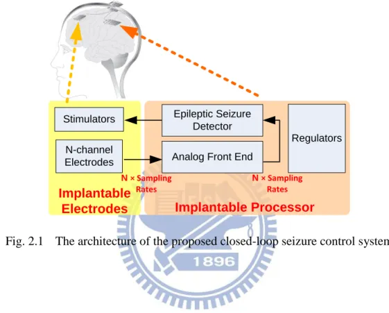
The closed-loop seizure control system contains implantable electrodes and an implantable processor including epileptic seizure detector and analog front end, as shown in Fig. 2.1. First, the EEG signals are delivered into analog front end by implantable electrodes. Then analog front end, which consists of amplifier, band-pass filter and A/D converter, transform the small and analog signals into digital data. Next, the epileptic seizure detector could perform continuous real-time detection and control stimulators. Finally, a 20-50μA constant current stimulation pulse is generated to restrain seizure from simulators.

In this study, the real-time closed-loop system scheme is based on large portion of epileptic seizure detector. Many technology can implement the digital seizure detector, such as digital signal processor (DSP), field-programmable gate array (FPGA), and application-specific integrated circuit (ASIC). DSPs have high processing capability but the large power is consumed by other hardware accelerators. Modern high-density FPGA combine embedded processor and custom hardware accelerator to achieve high performance;

however, it also consumes high static power cause of its advanced fabrication technology. ASIC is an integrated circuit which is highly specialized for a particular scenario or application. This solution is highly optimized in terms of area, power, and speed to perform its designated task. Therefore, ASIC is chosen in this research.

Analog Front End

Implantable Processor Regulators Implantable Electrodes Epileptic Seizure Detector Stimulators N-channel Electrodes N × Sampling Rates N × Sampling Rates

Fig. 2.1 The architecture of the proposed closed-loop seizure control system

2.1.1 Previous Work: 8051 Microcontroller

In our previous implementation, a wireless on-line seizure controller has been implemented with an enhanced 8051 microcontroller in freely moving subjects [13]. The seizure controller consisted of three modules: signal conditioning, microcontroller and stimulator. Spontaneous brain activities of the rat were amplified and band-pass filtered by the conditioning board. The core component on a microcontroller board was a CC2430 system-on-chip RF IC. The board was carried by each experimental subject, and a host computer for remote real-time monitors of spontaneous brain activities, while they were communicated based on a 2.4GHz wireless IEEE 802.15.4/ZigBee protocol.

8051 microcontroller was built up on single-channel, 200Hz sampling rate, 32MHz computing rate, and the execution time is 24.1ms. An 800Hz, 40% duty cycle, and 30-50146.19A stimulation pulse train for 0.5s was feedback to the rat to stop spontaneous SWDs. The 8051 microcontroller consumed 117.66mW, and the power consumption of such implementation was significant for implantable devices.

2.1.2 Multi-channel Closed-loop Epileptic Seizure Detector (MCESD)

In this research, the hardware of epileptic seizure detector for closed-loop seizure control is proposed. Fig. 2.2(a) illustrates the prototype system, which supports 2-channel EEG signals, is implemented in board level to verify real-time capability. A multi-channel closed-loop epileptic seizure detector (MCESD) receives EEG signals of rats through ADC and delivers a stimulus at seizure. The seizure detection algorithm is realized by MCESD, and the algorithm is detailed in Chapter 3. The hardware block diagram is shown in Fig. 2.2(b). 2-channel seizure detector is the main function of MCESD chip, and detail of four blocks are introduced in Chapter 4. CLKEN CLK MCESD ADC Pre-Amp Data[7:0] Stimulator EEG RESET Board STIM[1:0] Data Receiver I2C_ctrl[4:0] 2-channel Seizure Detector Clock Generator I2_{C Register} Bank (a) (b) Data Rate Channel EEG Signals

2.2

Materials

In order to develop an epileptic seizure controller, we have to understand the seizure type. The epilepsy detection algorithm is applied to absence seizures that is described in this section. In addition, the EEG signals are classified to five events, which are the materials for training animal’s model. Finally, the surgery details of rats are evaluated for animal test.

2.2.1 Seizure Types

Seizures are often associated with a sudden and involuntary contraction of a group of muscles and loss of consciousness. However, a seizure can also be as subtle as a fleeting numbness of a part of the body, a brief or long term loss of memory. Clinicians organize different types of seizure according to the source of the seizure within the brain. The two major seizures are partial seizures and generalized seizures. Partial seizures are divided on the extent to which consciousness is affected. If consciousness is unaffected, then it is a simple partial seizure; otherwise it is a complex partial seizure. Generalized seizures are classed according to the effect on the body, but all involve loss of consciousness. These include absence, myoclonic, clonic, tonic, tonic-clonic, and atonic seizures. Our experimental rats with absence seizures are Long-Evans rats, so absence seizures is introduced in this study.

Absence seizure — also known as petit mal — involves a brief, sudden lapse of consciousness. Absence seizures are more common in children than adults. Someone having an absence seizure may look like he or she is staring into space for a few seconds. The difference between absence seizure and normal trance is that someone made a response immediately from external impetus when he or she was in a trance; however, the patient

didn’t answer until a absence seizure ended. Absence seizures appear mild compared with other types of epileptic seizures, but they can be dangerous. Children must be supervised carefully while swimming or bathing because of the danger of drowning. Teens and adults may be restricted from driving and other potentially hazardous activities.

Absences seizures are brief, generalized epileptic seizures of sudden onset and termination. They have 2 essential components: clinically the impairment of consciousness and EEG generalized spike-and-slow (SWD) wave discharges. The time–frequency structure of SWDs contains important information about the mechanisms of this type of brain paroxysmal activity. The frequency of SWD in patients with absence epilepsy is typical in the range of 3-5Hz [14, 15].

2.2.2 Animal Preparation

The genetic defect of Long-Evans rats causes spontaneous SWD, so adult Long-Evans rats with spontaneous spike-and-wave discharges (SWDs) were used in the study. The EEG characteristic of spontaneous SWD is much more close to epileptic patients’ EEG in the clinical aspect. The animals were kept in a room under a 12:12-hour light-dark cycle with food and water provided ad libitum. All surgical and experimental procedures were reviewed and approved by the Institutional Animal Care and Use Committee of the National Cheng Kung University.

The rats were anesthetized with sodium pentobarbital (50mg/kg, i.p.). Subsequently, it was placed in a standard stereotaxic apparatus. Screw electrodes were bilaterally implanted over the area of the frontal barrel cortex (anterior 2.0mm, lateral2.0 mm with regard to the bregma). A four-microwire bundle, each made of Teflon-insulated stainless steel microwires

(#7079, A-M Systems), was used to stimulate the right-side zona incerta (ZI). A ground electrode was implanted 2mm caudal to the lambda. Dental cement was applied to fasten the connection socket to the surface of the skull. Following suturing to complete the surgery, animals were given antibiotics and housed individually in cages for recovery.

Two weeks after the surgery, each animal was placed in the recording environment at least two times (1 hour/day) prior to testing. In this procedure, about 90% of Long-Evans rats show spontaneous SWDs, which were used for continuous EEG recording. Continuous EEGs from 5 hours to 24 hours (contained one circadian cycle) were recorded and analyzed to assess our seizure detector in this study.

2.2.3 Continuous EEG Recording

(a)WK

(b)SWD

(c)SWS

(d)Artifact

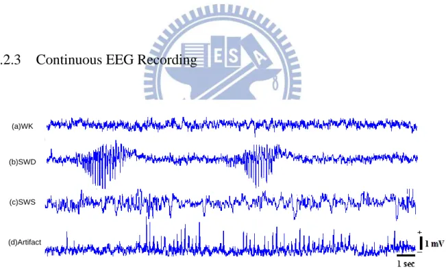
Fig. 2.3 All kinds of EEG patterns in a continuous recording of a Long-Evans rats

In order to develop high accuracy of a seizure detection system, the controller must be powerful enough to avoid false alarms caused by various activities. Fig. 2.3 shows all kinds of EEG patterns in a continuous recording of a Long-Evans rat. (a) and (b) are wakefulness (WK), spike-and-slow wave discharges (SWDs) respectively. We could observe obvious

shake-up waves in EEG signal. Slow-wave sleep (SWS) and movement artifact are included in (c) and (d) respectively.

Two essential stages of EEG signal processing were executed in Long-Evans rats. In the first stage, continuous EEG signals of each rat were recorded without providing electrical stimulation, and the data were classified according to seizures (SWD) and non-seizures (WK, SWS, and artifact) for feature extraction. These spontaneous events were used to off-line training and got the parameters of a seizure detection model. The second stage, optimal parameters is loaded into seizure detector at initial. The rats went through an on-line closed-loop seizure controller with immediate feedback and electrical stimulation.

Chapter 3

Epileptic Seizure Detection Algorithm

The seizure detection algorithm is realized by MCESD. The chapter illustrate the four parts of algorithm, entropy analysis, spectral analysis, linear least squares, and adaptive threshold, respectively. In addition to the algorithm, experimental flow is described in the end of this chapter.

3.1

Detection Algorithm

The seizure detection algorithm is realized by MCESD. Fig. 3.1 shows the flow of the algorithm. In this algorithm, the sampling rate is 200Hz (5ms), and 64-point EEG data is defined a sampling window (0.32s) with 50% overlap, in Fig. 3.2. The 64-point window is to reduce the detection delay time and inspirit quick seizure detection.

EEG Data Evaluate S1 and S2 Evaluate CM Entropy Analysis 64-point Short-Term Fourier Transform Spectral Analysis Linear Least Squares (LLS) and Seizure Detection Stimulator

The Seizure Detection Algorithm

Adaptive Threshold

EEG Signals

5ms A Sampling Window

Time

A Sampling Window A Sampling Window 32 points (0.16s) 64 points (0.32s)

Fig. 3.2 A sampling window include 64 EEG data with 50% overlap

The time-domain and frequency-domain characteristics of EEG signals were integrated as the features and the linear least square (LLS) model was utilized to implement seizure classifier. Entropy has been used for seizure because the EEG pattern of a seizure is more regular than that in normal states [16]. According to the animal test, the absence seizure has large power at 7-9 Hz and 14-18Hz [17]. The fast Fourier transform (FFT) was used to calculate powers of frequency bands. Therefore, EEG band powers were combined to ApEn analysis to improve the performance of epileptic seizure detection. Because the objects’ seizure conditions are different, we need to train the optimal parameters by EEG of subjects through an off-line process. The three features and the parameters of LLS classifier compute at on-line seizure detector [18].

3.1.1 Complexity Analysis

According to the phenomenon that the EEG signals of a seizure is more regular than that in normal states, entropy has been used for analysis and detection. Approximate entropy (ApEn) is a measure, quantifying a time series of signals and is therefore a preferred measure of randomness or regularity.

Approximate entropy

First, given a time-series of data u(1), u(2),. . . , u(N), from measurements equally spaced in time, forming a sequence of vectors x(1), x(2), . . ., x(N-m+1) in Rm, defined by x(i) = [u(i),

u(i+1), . . ., u(i+m-1)] for 1≤ i ≤ N-m+1, where N is the window size, and m is the compared

length. Then, We must define d[x(i), x(j)] for vectors x(i) and x(j). The two vectors compare each element. For each i and j, 1≤ j , i ≤ N-m+1.

1,2,..., 1 [ ( ), ( )] max (| ( ) ( ) |) k m d x i x j u i k u j k       _(3.1) 1 1 1, [ ( ), ( )] ( ) 0, 1 N m j j m i j if d x i x j r C r else N m         _{ }   _



(3.2)

where r is the tolerance of d. Finally, the approximate entropy is calculated by

1 1 ln ( ) ( ) 1 N m m i m i C r r N m       



_(3.3) 1 ( , , ) m( ) m ( ) ApEn m r N   r   r (3.4) CM Entropy

A simplified measurement based on the ApEn is proposed to reduce the computational cost, so we define a complexity measurement, CM.

1 1 ( ) 1 N m m i m i C r S N m      



_(3.5) 1 m m m S CM S   (3.6)

The average of r is 5 for Long-Evan rats which is determined in off-line training, but in fact it’s variable for each object. Therefore, we could define the four steps to calculate the CM,

as shown in Fig. 3.3 . The first step is to load EEG signals. Although we define the sampling window size is 64-point EEG before, at this step the entropy window is divided to four parts,

N= 16, to decrease the complicated of algorithm, as shown in Fig. 3.4. Besides, the parameter

setting is m=1.

Load EEG Evaluate Decision Bits (ωj)

Evaluate S1 and S2

Evaluate CM

Fig. 3.3 The Entropy Extraction Flow

32 33 34 35 … … 60 61 62 63 28 29 30 31 0 1 2 3 … … 0 60 1 5 2 6 3 7 4 61 62 63 … Part 1 Part 2 Part 3 Part 4 32 33 34 35 … … … … … … … 36 37 38 39 40 41 42 43 16 points

Fig. 3.4 The 64-point window is divided to four parts

The second step evaluates decision bit (ωj), and next step evaluates S1 and S2. The

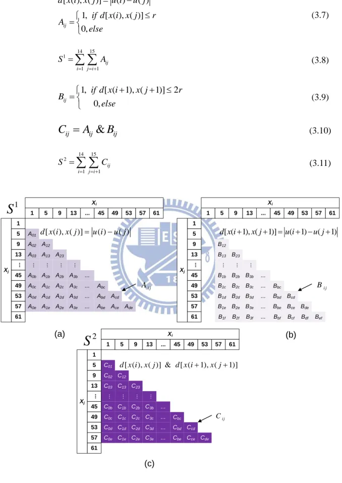
equations are (3.7) to (3.10). The decision bits are shown in Fig. 3.5, in which (a) correspond to d[x(i), x(j)]= |u(i) – u(j)|; (b) correspond to d[x(i+1), x(j+1)]= |u(i+1) – u(j+1)|. If the comparison distance between data is less than a threshold (r), decision bits are set to be logic 1; else are set to be logic 0. The decision bits, Aij, Bij, and Cij are one bits (0 or 1), and Cij

equate Aij& Bij in equation (3.10) which correspond to d[x(i), x(j)]= max| u(i) – u(j), u(i+1) –

u(j+1)|, in Fig. 3.5(c). S1 is evaluated by A01 to Ade, and S2 is evaluated by C01 to Cde. Then, the

CMp is evaluated by S2/ S1 for p = 1, 2, 3, 4. Finally, the CM is evaluated by four CMp, which ranging from 0 to 4.

[ ( ), ( )] ( ) ( ) 1, [ ( ), ( )] 0, ij d x i x j u i u j if d x i x j r A else        (3.7) 14 15 1 1 1 ij i j i S A    

 

_(3.8) 1, [ ( 1), ( 1)] 2 0, ij if d x i x j r B else        (3.9)

&

ij ij ij

C



A

B

(3.10) 14 15 2 1 1 ij i j i S C    

 

_(3.11) .. . [ ( ), ( )] ( ) ( ) d x i x j  u i u j 1 5 9 13 ... 45 49 53 57 61 Xi Xj A01 A02 A03 A0b A0c A0d A0e 1 5 9 13 .. . 45 49 53 57 61 A12 .. . _... _... A13 A1b A1c A1d A1e A23 A2b A2c A2d A2e A3b A3c A3d A3e ... ... ... ... Abc Abd Abe Acd Ace Ade 1 5 9 13 ... 45 49 53 57 61 Xi Xj 1 5 9 13 .. . 45 49 53 57 61 B12 .. . _... _... B13 B1b B1c B1d B1e B23 B2b B2c B2d B2e B3b B3c B3d B3e ... ... ... ... Bbc Bbd Bbe Bcd Bce Bde [ ( 1), ( 1)] ( 1) ( 1) d x i x j  u i u j .. . 1 5 9 13 ... 45 49 53 57 61 Xi Xj C01 C02 C03 C0b C0c C0d C0e 1 5 9 13 .. . 45 49 53 57 61 C12 .. . _... _... C13 C1b C1c C1d C1e C23 C2b C2c C2d C2e C3b C3c C3d C3e ... ... ... ... Cbc Cbd Cbe Ccd Cce Cde [ ( ), ( )] & [ ( 1), ( 1)] d x i x j  d x i x j (a) (b) (c) i j A B_{i j} ij C B1f B2f B3f ... Bbf Bcf Bdf Bef 1

S

2

S

However, the sleep signal is similar to seizure signals at time-domain, because those signals revealed a rhythmic-like pattern. Fig. 3.6 shows the results of entropy. According to Fig. 3.6(c) and (d), the entropy result of SWS and artifact are instable. Thus, to improve the performance, spectral features combine with entropy analysis.

Fig. 3.6 Entropy values in different behavioral states (a) WK, (b) SWD, (c)SWS, and (d) Artifact

3.1.2 Spectral Analysis

The fast Fourier transform (FFT) is used to calculate powers of frequency bands, and it is well-established in various microprocessor. Fig. 3.7 shows the methods to build the correlation between time domain and frequency domain. In time domain, seizure events are set to one, or else are set to zero. The vectors are correlated with powers of specific frequency bands. In this algorithm, we use Pearson correlation coefficient to determine spectral features. Consider there are k segments, and let SPk (t,f) be the spectrogram of the kth segment. Define

xk(m) as the spectrum index which is the spectrogram in frequency m. Then, define y as the

SWD index. The correlation coefficient Corrk(m) of the seizure index and spectrum index is

given by (3.14). Finally the average correlation coefficient of k segments is given by (3.15). ( ) [ (1, ), (2, ),...] k k k x m SP m SP m (3.12) 1, [ (1), (2),...] ( ) 0, k k k k

if the state in time t is seizure

y t else







  _{ }  (3.13) 2 2 ( ( ) ( )) ( ) ( ) ( ( ) ( )) ( ) k k k k k k k k k x m x m y y Corr m x m x m y y       







(3.14) ( ) ( ) k k Corr m C m k 



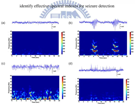
(3.15)

The absence seizure has large power at first harmonic (7-11 Hz) and second harmonic (14-18 Hz). Sleep states contain delta rhythms and have large power under 4Hz. Artifact does not have large power obviously. Fig. 3.8 shows the spectrogram in four states of time-frequency analysis, which based on short-term Fourier transform. Therefore, spectral analysis is combined to entropy analysis to improve the performance of epileptic seizure detection [17, 19-21]. In this study, three frequency bands (0-4Hz, 7-11Hz, and 15-18Hz) are selected as spectral indexes.

Correlation coefficient Corrk(m) F re q u e n c y Spectrogram EEG Seizure index yk(m) Spectral index xk(m) 0 1 0 Time m Time kth SWD segment

Fig. 3.7 Seizure event and a particular frequency band combine to identify effective spectral indexes for seizure detection

Fig. 3.8 The five behavioral states of time-frequency analysis (a) AW, (b) absence seizures, (d) SWS, and (e) Artifact

3.1.3 Linear Classifier

Because the objects’ seizure conditions are different, the algorithm must have flexible model by EEG of subjects. The linear least squares (LLS) method is used to find a best fitting linear model. LLS is the problem in approximately solving an over-determined system of linear equations, where the best approximation is defined as that which minimizes the sum of squared differences between the data and the desired data. Besides, the method could reduce the computational cost for implementation, because the model output is only the weighted sum of the input.

At first, consider an over-determined system (3.16), m is number of data pair for training in n coefficients. yi is the output of LLS. βj is the weight parameter. This can be written in

matrix form as (3.17). The residual is the difference between the observed value and the value calculated by the model (3.18). Next, S is minimized when its gradient vector is zero. The elements of the gradient vector are the partial derivatives of S with respect to the parameters (3.19). We obtain the normal equations (3.20), and the  is minimizes S. Finally, the normal equations are written in matrix notation as (3.21). Thus, the solution of the normal equations yields the vector of  the optimal parameter values (3.22).

1 , 1, 2,..., n i ij j j y X  i m  



 _(3.16) 1 11 12 1 1 2 21 22 2 2 1 1 n n m m m mn n y X y X X X y X X X y X y X X X                                              (3.17) 2 1 1 ( ) m n i ij j i j S  y X       _  _  





(3.18)

1 1 2 ( ) 0 , 1, 2,..., m n ij i ij k i k i S X y X  j n     _{    } 





(3.19) 1 1 1 ˆ m m m ij j ij ik k i i k X y X X     





(3.20) ˆ ( T ) T X X  X y (3.21) 1 ˆ ₍ T ₎ T X X X y  _  (3.22)

In this study, LLS is used in two stages. The first stage is off-line training. Three feature indexes, which are CM, band 1 (7-1Hz), and band 2 (17-22Hz), are input into classifier to verify seizure occurrences. The target output values are zero for non-seizure windows, and one for seizure windows. Therefore, the equation (3.17) can be written to (3.23), and used (3.22) to find the best model β for each subject. The second stage is on-line computing. Optimal parameters ware determined at last stage, which compute with three features at on-line seizure detector (3.24).

1 2 1 1 1 2 2 2 0( ) 1( ) 1 0 1 2 1 1 2 1 1 2 1 CM Band Band Const m m m non seizure seizure y or CM Band Band CM Band Band X CM Band Band                                              (3.23) 1 2 1 2

on line CM Band Band Const

3.1.4 Adaptive Threshold

Because the entropy analysis of SWS state usually leads to false detection easily, but the state has large power less than 4Hz, an adaptive threshold is proposed to decrease the false alarms. Adaptive threshold is to switch the threshold of LLS between SWS state and SWD state. According to Fig. 3.6 and Fig. 3.8, although the SWS signals resemble with SWD signals at time-domain, the frequency power of SWS has an oscillation within delta frequency range (0.5-4Hz). Therefore, the frequency band 0 is used to determine the SWS state. If band 0 has higher energy than a threshold of sleep (Thsws), the threshold of LLS is switched to a

higher value to avoid the false alarms. Equation (3.25) shows an adaptive threshold. At training stage, average band0 of the sleep EEG minus or plus standard deviation of the sleep EEG (3.26). Thwake is decided by the LLS result of seizure event, and Thsleep is based on the

LLS result of seizure event in SWS state, (3.27). Fig. 3.9 shows the false detection without adaptive threshold. , , , 0 , wake Th sleep sws

Th otherwise Wake state

LLS

Th if Band Th Sleep state



  _

 (3.25)



0





0



sws

Th mean Band Std Band (3.26)









sleep sws sws

Th mean LLS Std LLS (3.27)

In addition, the window constraint is set to avoid the influence of EEG signals. If the LLS classifier output is larger than the LLSTh in consecutive three 32-sample, the seizure

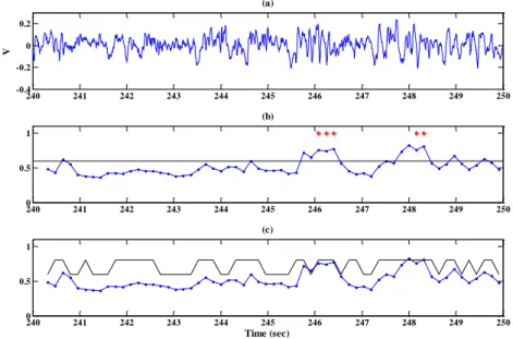
event is detected. Therefore, the delay time of seizure detection is 0.48s least (5ms×32×3), but it is the tolerable delay time to restrain seizure. Fig. 3.10 shows the seizure detection algorithm include three features and Band 0.

Fig. 3.9 Non-adaptive and adaptive threshold of SWS: (a) EEG signal, (b) without adaptive threshold, (c) adaptive threshold

Fig. 3.10 (a) EEG signals, (b) CM, (c) Band 0, (d) Band 1, (e) Band 2

240 241 242 243 244 245 246 247 248 249 250 -0.4 -0.2 0 0.2 (a) V 240 241 242 243 244 245 246 247 248 249 250 0 0.5 1 (b) 240 241 242 243 244 245 246 247 248 249 250 0 0.5 1 (c) Time (sec)

3.2

Experimental Flow

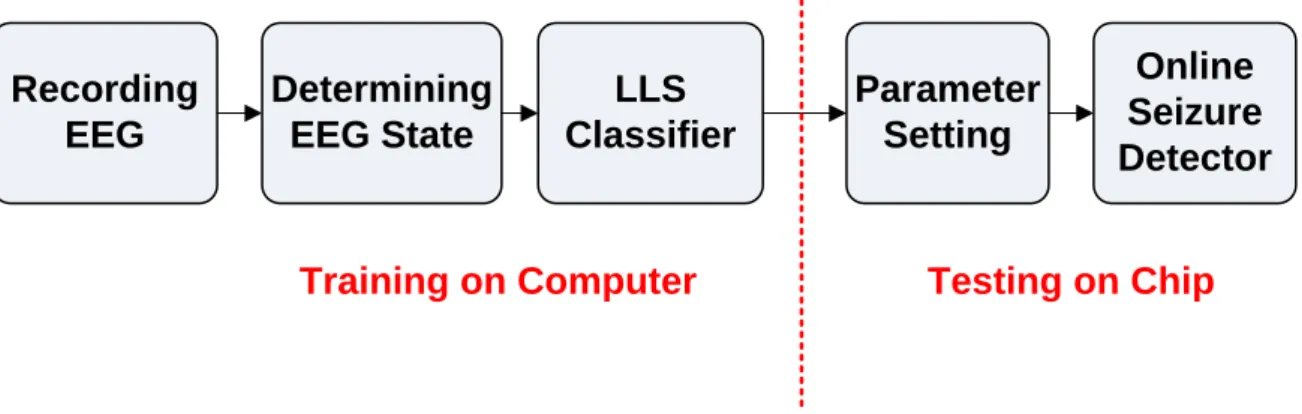
Recording EEG Determining EEG State LLS Classifier Parameter Setting Online Seizure Detector

Training on Computer Testing on Chip

Fig. 3.11 Experimental flow

To make sure the seizure detector is useful, experimental flow is divided into five stages, in Fig. 3.11. The first stage is recording EEG data. In this study, the long-term recording is five hours and twenty-four hours of continuous EEG data without electrical stimulation. The second stage is determining EEG state. After recording the EEG data, the EEG data is distinguished behavioral states by experts. The spontaneous events include AW, SWD, SWS, and artifact. The first stage and the second stage are both executed at the Institutional Animal Care and Use Committee of the National Cheng Kung University.

Next stage is LLS classifier. For finding the best model of objects, LLS classifier is utilized by Matlab. In the train step, seizure and non-seizure segments with equivalent length are selected for LLS model, and the ratio of non-seizure segments including WK, SWS, and artifice are 1:1:1, as shown in Fig. 3.12. Two hours of three feature indexes are trained to get a pair of parameters, and those parameters is testing five hours of EEG data. When the detection accuracy is above 92%, the parameters are applied to on-line stage, else data is trained repeatedly.

Then, the optimal parameters are downloaded to MCESD chip by I2C interface at initial stage. I2C interface will be described in next section. Finally, the online seizure detector is developed to seizure detection.

Seizure AW SWS Artifact

1:1

1:1:1

Chapter 4

Design and Implementation

According to Fig. 2.2, the block diagram shows four blocks in MCESD chip, including 2-channel seizure detection, I2C register bank, data receiver, and clock generator. The first part, 2-channel seizure detector implements the seizure detection algorithm. The computing rate is 3.2 kHz. MCESD needs to generate the control signal and clock for different ADC circuits, so the second part and third part are clock generator and data receiver, which synchronized ADC signal and generated the clock for seizure detector (3.2kHz). The last part is I2C register bank, which loads the parameters to system at initial, and saves the value of seizure detector for verifier function.

4.1

2-channel Seizure Detector

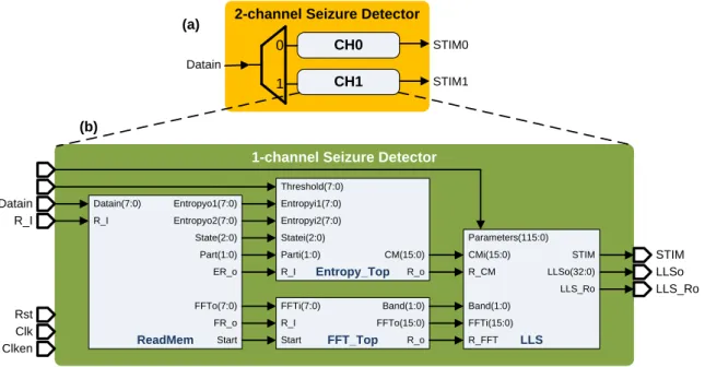
In Chapter 3, the seizure detection algorithm is described in detail, and it is implemented in the 2-channel seizure detector. Fig. 4.1 shows the block diagram of seizure detector. The 2-channel seizure detector is composed of two 1-channel seizure detector, and a switch determining that data are delivered to channel 0 or channel 1, as shown in Fig. 4.1(a).

Fig. 4.1 (b) illustrates the blocks of 1-channel seizure detector which correspond with the algorithm. Clk means clock of detector. In this block, the computing clock is 3.2kHz (200Hz ×16). Because the sampling clock is 200Hz, and the entropy window size is 16-point, 3.2kHz is the lowest clock of computing to handle the data in real-time. Rst is 1 in normal state, and all registers are cleared when Rst is 0. Clken is clock enable; the system is paused when Clken is set to 0. The block detail will be introduced in following section. Clk, Clken, and Rst all connect to each block.

1-channel Seizure Detector 2-channel Seizure Detector

CH0 CH1 0 1 Datain STIM0 STIM1 Datain(7:0) R_I Entropyo1(7:0) Entropyo2(7:0) State(2:0) Part(1:0) ER_o FFTo(7:0) Start FR_o Entropyi1(7:0) R_I CM(15:0) R_o Entropyi2(7:0) Statei(2:0) Parti(1:0) Threshold(7:0) ReadMem Entropy_Top R_I FFTo(15:0) R_o FFTi(7:0) Start FFT_Top Band(1:0) CMi(15:0) R_CM Band(1:0) FFTi(15:0) R_FFT Parameters(115:0) LLS STIM LLSo(32:0) LLS_Ro Datain R_I Rst Clk Clken STIM LLSo LLS_Ro (a) (b)

Fig. 4.1 Block diagram of seizure detector (a) 2-channel detector (b) one channel detector

4.1.1 Read Memory

Datain(7:0) R_I Entropyo1(7:0) Entropyo2(7:0) State(2:0) Part(1:0) ER_o FFTo(7:0) Start FR_o ReadMem

Fig. 4.2 Interface of read memory

This block receives EEG data and saves data, than it feds data to entropy block and FFT block. Read memory contains a 2-port 128×8 memory. An input port of memory writes the Datain into memory when the R_I is set to 1, and the other is unused. One output port is for entropy, and the other is for FFT. Entropyo1 is output which correspond to u(i) – u(j); Entropyo2 corresponds to u(i+1) – u(j+1). Because the 64-point is divided into four segments,

Part is display the segments, and State is show the order of the 16-point data. On the other hand, there are three signals for FFT block. Start is used to wake up the FFT block to be ready for received FFT data, and FFTo will deliver continuous data to next block. ER_o and FR_o are set to 1, which means the data are ready to be delivered. All inputs and outputs are shown in Fig. 4.2.

4.1.2 Entropy Extractor

Entropyi1(7:0) R_I CM(15:0) R_o Entropyi2(7:0) Statei(2:0) Parti(1:0) Threshold(7:0) Entropy_Top

Fig. 4.3 Interface of entropy extractor

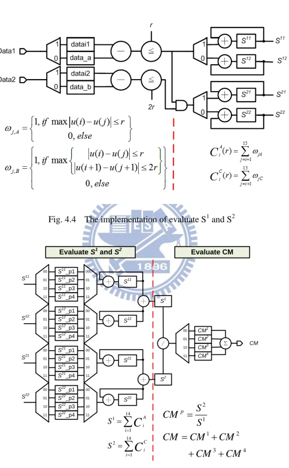
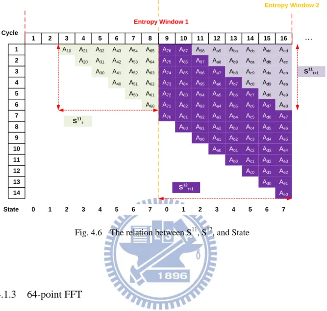
Fig. 4.3 shows the input and output of entropy extractor, and the threshold is equal to "r". The inputs (Entropyi, Statei, Parti, and R_I) are connected with outputs of ReadMem (Entropyo, State, Part, and ER_o), and CM is output. Fig. 4.4 and Fig. 4.5 illustrate the hardware implementation of entropy extractor. First, u(i)–u(j) and u(i+1)–u(j+1) are implemented with two subtracters, and decision bits (ωj) are decided that the values compare

with r and 2r. Next, accumulators save the decision bits, and S1 t+1= S11t +S12t+1 + S11t+1, S2 t+1 is

also. The detail of S11 and S12 is shown in Fig. 4.6. A divider computes S2/S1. The complexity measurement is sun of CMp. The output of CM is 4-bit unsigned integer and 12-bit fractional.

Fig. 4.4 The implementation of evaluate S1 and S2 S11_p1 S11_{_p2} S11_{_p3} S11_{_p4} 00 01 10 11 S12_{_p1} S12_{_p2} S12_{_p3} S12_p4 00 01 10 11 S21_{_p1} S21_p2 S21_p3 S21_p4 00 01 10 11 S22_p1 S22_p2 S22_p3 S22_p4 00 01 10 11 11 10 01 00 11 10 01 00 11 10 01 00 11 10 01 00 S11 S12 ┼ S21 ┼ S22 ┼ ┼ ┼ S1 S2 ∕ 00 01 10 11 CM1 CM2 CM3 CM4 Σ CM ┼ Evaluate CM Evaluate S1 and S2 S22 S21 S12 S11 14 1 1 14 2 1 A i i C i i S S

C

C

   





2 1 1 2 3 4 p

S

CM

S

CM

CM

CM

CM

CM











A10 1 A32 A43 A20 A21 A30 2 3 4 5 7 8 9 10 11 Cycle 6 12 13 14 A31 A42 A41 A40 A53 A52 A51 A50 A54 A63 A62 A61 A60 A64 A65 Entropy Window 2 A73 A72 A71 A70 A74 A75 A76 A83 A82 A81 A80 A84 A85 A86 A87 A93 A92 A91 A90 A94 A95 A96 A97 A98 Aa9 Aa8 Aa3 Aa2 Aa1 Aa0 Aa4 Aa5 Aa6 Aa7 Ab9 Ab8 Ab3 Ab2 Ab1 Ab0 Ab4 Ab5 Ab6 Ab7 Aba Ac9 Ac8 Ac3 Ac2 Ac1 Ac0 Ac4 Ac5 Ac6 Ac7 Aca Acb Ad9 Ad8 Ad3 Ad2 Ad1 Ad0 Ad4 Ad5 Ad6 Ad7 Ada Adb Adc Ae9 Ae8 Ae3 Ae2 Ae1 Ae0 Ae4 Ae5 Ae6 Ae7 Aea Aeb Aec Aed 1 2 3 4 5 6 7 8 9 10 11 12 13 14 15 16 S11t S12t+1 S11t+1 Entropy Window 1 … 1 2 3 4 5 6 7 0 State 0 1 2 3 4 5 6 7

Fig. 4.6 The relation between S11, S12, and State

4.1.3 64-point FFT

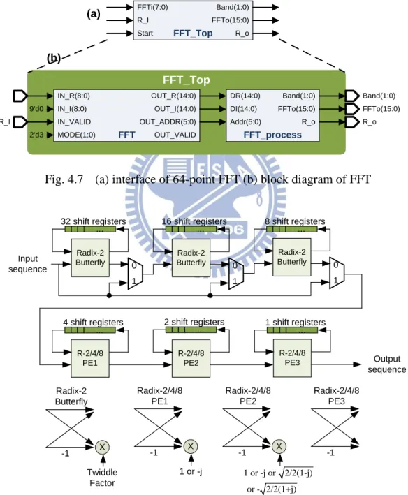
The overview of the 64-point FFT is shown in Fig. 4.7, including FFT main function and FFT_process. FFT is a core from SoC Design Lab, Instituation of Communication Engineering, NCTU, which supports 9-bit signed complex input and 15-bit signed complex output. Four modes are selected, because the FFT core could compute 8, 16, 32, and 64 size of FFT. In this study, the size of FFT are always 64 points, so mode is fix value. When the IN_VALID is high, the data will deliver the data to do the computation. Due to EEG signals is real numbers, imaginary numbers are zero.

The architecture of 64-point radix-2/4/8 FFT is shown in Fig. 4.8, and the main advantage of radix-2/4/8 is reducing number of complex multipliers. Fig. 4.9 shows the signal

flow of 64-point radix-2/4/8 FFT [22]. Fixed multiplicand like ±j and 2/2(1 j) are used to replace complex multipliers. Therefore, the algorithm apply to length of 8n FFT and decrease the computational cost. Consider to the SQNR is achieve 30dB, so the bit of output increase 2 bits at radix-2 butterfly stages. Then, the least three stage fix the bit number to retrench area. Twiddle factor is used one bit integer and sixteen bits fractional.

FFT_Top R_I FFTo(15:0) R_o FFTi(7:0) Start FFT_Top Band(1:0) IN_R(8:0) IN_I(8:0) IN_VALID MODE(1:0) OUT_R(14:0) OUT_I(14:0) OUT_ADDR(5:0) OUT_VALID FFT DR(14:0) DI(14:0) Addr(5:0) Band(1:0) FFTo(15:0) R_o FFT_process 9'd0 2'd3 R_I Band(1:0) FFTo(15:0) R_o (a) (b)

Fig. 4.7 (a) interface of 64-point FFT (b) block diagram of FFT

Radix-2 Butterfly 32 shift registers 1 or -j -1 Radix-2 Butterfly Radix-2/4/8 PE1 X Twiddle Factor ... 0 1 Radix-2 Butterfly 16 shift registers ... 0 1 Radix-2 Butterfly 8 shift registers ... 0 1 Input sequence R-2/4/8 PE1 4 shift registers ... R-2/4/8 PE2 2 shift registers ... R-2/4/8 PE3 1 shift registers ... Output sequence -1 X Radix-2/4/8 PE2 -1 X Radix-2/4/8 PE3 -1 1 or -j or 2/2(1-j) or - 2/2(1+j)

X[0] X[1] X[2] X[3] X[4] X[5] X[6] X[7] … … … … … … … … … … … … … … … … … … … … … … … … … … … X[56] X[57] X[58] X[59] X[60] X[61] X[62] X[63] r-2 r-2/4 r-2/8 1 2 3 Stage r-2 r-2/4 r-2/8 r-2 r-2/4 r-2/8 r-2 r-2/4 r-2/8 r-2 r-2/4 r-2/8 r-2 r-2/4 r-2/8 r-2 r-2/4 r-2/8 r-2 r-2/4 r-2/8 r-2 r-2/4 r-2/8 4 5 6 X[0] X[31] X[16] X[48] X[8] X[30] X[24] X[56] … … … … … … … … … … … … … … … … … … … … … … … … … … … X[7] X[39] X[23] X[55] X[15] X[47] X[31] X[63]

Fig. 4.9 Signal flow of 64-point radix-2/4/8 FFT

FFT_process calculates power of specific frequency bands by spontaneous brain waves. FFT output is DR+DIj, and the power of FFT is means |FFTo| DR2DI2 . The input of DR and DI are 16 bits signed integer, and ADDR display the frequency of FFT. When the address is 0, 4, and 7 which correspond with Band0, Band1, and Band2, the FFTo are computed. The output of FFTo is 9-bit unsigned integer and 7-bit fractional. Fig. 4.10 illustrates the hardware implementation of FFT_process.

FFT_Process 0 1 DR DI + 1 0 Add1 Add2 + 2 2 |FFTo| DR DI ADDR DR DI FFTo

Fig. 4.10 The implementation of FFT_process

4.1.4 LLS Classifier

CMi(15:0) R_CM Band(1:0) FFTi(15:0) R_FFT Parameters(115:0) LLS STIM LLSo(32:0) LLS_Ro

Fig. 4.11 Interface of LLS Classifier

Fig. 4.11 shows the input and output ports of LLS block. Input acquire data by last stage, and the parameters are input from I2C register bank, which detail is on next section. LLSo will save into I2C register bank to check the values. In the training phase, the large matrix are used to training on computer, but the hardware implementation on chip just need three features from previous blocks and the parameters in registers. Band 0 is a condition to switch the

LLSTh. Fig. 4.12 illustrate the hardware implementation of LLS. First, LLS out is calculated

by the input. Next, the seizure detection counter is incremented when a seizure occur; otherwise, the counter is zero. If the counter reaches DET_WINDOW, STIM, a flag of stimulation is set, and the flag keep DET_STIM×0.16 seconds. The optimal parameters' detail is shown in Table 4.1, and the default values of DET_WINDOW and DET_STIM are 3.

CM

Band1

Band2

X

+

LLS

Paramters

MUX

LLS

on-line

Band0

Adaptive Threshold

If (DETSWS_TH_HIGH > Band0 > DETSWS_TH_LOW ) LLSTh = [(LLS_COEF_CONST1- DETSWD_TH_SWS), LLS_COEF_CONST2 ]

Else If (Band0 < DETSWS_TH_LOW)

LLSTh = [LLS_COEF_CONST1, LLS_COEF_CONST2] Stimulation Scheme

STIM

Adaptive Threshold LLSTh

LLSon-line = CM × LLS_COEF_CM + Band1 ×

LLS_COEF_BAND1 + Band2 × LLS_COEF_BAND2

Stimulation Scheme

If (LLSon-line - LLSTh> 0, Continuous DET_WINDOW times) Enable Stimulator , and continue DET_STIM × 0.16 seconds

Table 4.1 Specifics of features and parameters

Name Integer (bits) Fractional (bits) Default Value

Features CM 4 12 N/A Band0 9 7 N/A Band1 9 7 N/A Band2 9 7 N/A Parameters THRESHOLD(r) 8 0 5 LLS_COEF_CM 12 4 N/A LLS_COEF_BAND1 7 9 N/A LLS_COEF_BAND2 7 9 N/A LLS_COEF_CONST1 16 0 N/A LLS_COEF_CONST2 0 16 N/A DETSWD_TH_SWS 16 0 N/A DETSWS_TH_LOW 9 7 N/A DETSWS_TH_HIGH 9 7 N/A DET_WINDOW 4 0 3 DET_STIM 4 0 3 LLSTh 16 16 N/A LLSon-line 17 16 N/A

4.2

I

2

C Register Bank

Because there are many parameters is need to set in MCESD chip at initial, I2C interface is used to save numbers of pad. Inter-integrated circuit register bank (I2C register bank) is an interface integrated with 8-bit×N register bank for sub-circuit configuration, and 8-bit×M inputs for sub-circuits status readout [23]. The block diagrams are shown in Fig. 4.13. Control pins of target sub-circuits can be reduced to only 3 pins (sda, saddr and scl), because clk and reset are integrated with 2-channel seizure detector. The pins are controlled by I2C master, as shown in Fig. 4.14.

Scl is a clock signal, and being utilized for synchronizing I2C data input. Sdain, Sdaout, Oe are the data and direction control pin for bidirectional pad. Saddr is used for I2C slave identification. In this case, only less significant bit is connected out, and the other two pins are set to zero. ctrl0 – ctrlN are 8-bit×64 registers and they connect to 2-channel seizure detector for configuration purpose. readin0 – readingM are 8-bit×64 reading registers for 2-channel seizure detector status readout purpose. Table 4.2 shows the relation between seizure detector and I2C register bank.

I2C Register Bank Rst In(7:0) Scl Saddr(0) Sdain Clk I2C Slave Interface out(7:0) Oe Sdaout out_en addr_reset rw_out in_strobe Inv_sdaout Rst ctrl0(7:0) rb_out(7:0) rb_in(7:0) rbin_en Clk Register Bank . rw addr_reset ctrlN(7:0) readin0(7:0) rbout_strobe . . readinM(7:0) . . . . . . . . . 2-channel Seizure Detector 3'd0 CLK RST SCL SDA Saddr(2:1) SADDR

Fig. 4.13 The block diagrams of the I2C register bank

Table 4.2 Parameters of MCESD correspond with I2C register bank

Parameters I2C Register (8bits)

Parameters I2C Register (8bits)

Clock Generator CH1_LLS_COEF_CONST1 ctrl29,ctrl28 DIV_3200 ctrl1[3:0],ctrl0 CH1_LLS_COEF_CONST2 ctrl31,ctrl30 DIV_500K ctrl1[7:4] CH1_DETSWD_TH_SWS ctrl33,ctrl32 MODE ctrl2[1:0] CH1_DETSWS_TH_LOW ctrl35,ctrl34 CH0 Parameters CH1_DETSWS_TH_HIGH ctrl37,ctrl36 CH0_THRESHOLD(r) ctrl3 CH1_DET_WINDOW ctrl38[3:0] CH0_LLS_COEF_CM ctrl5,ctrl4 CH1_DET_STIM ctrl38[7:4] CH0_LLS_COEF_BAND1 ctrl7,ctrl6 CH0 Results

CH0_LLS_COEF_BAND2 ctrl9,ctrl8 CH0_FFTo readin1,readin0

CH0_LLS_COEF_CONST1 ctrl11,ctrl10 CH0_CMo readin3,readin2 CH0_LLS_COEF_CONST2 ctrl13,ctrl12 CH0_LLSo readin8[0],readin7

,readin6,readin5 ,readin4 CH0_DETSWD_TH_SWS ctrl15,ctrl14 CH0_DETSWS_TH_LOW ctrl17,ctrl16 CH0_DETSWS_TH_HIGH ctrl19,ctrl18 CH0_R_LLS readin8[1] CH0_DET_WINDOW ctrl20[3:0] CH1 Results

CH0_DET_STIM ctrl20[7:4] CH1_FFTo readin10,readin9

CH1 Parameters CH1_CMo readin12,readin11

CH1_THRESHOLD(r) ctrl21 CH1_LLSo readin17[0],readin16

readin15,readin14, readin13 CH1_LLS_COEF_CM ctrl23,ctrl22

CH1_LLS_COEF_BAND1 ctrl25,ctrl24

4.3

Clock Generator and Data Receiver

RST CLKEN MODE(1:0) DIV_3200(11:0) DIV_500K(3:0) CLK Clock Generator CLK_OUT CLK_500K CLK_3200 RST CLKEN R_I CLK Data Receiver CHANNEL R_Ix (a) (b)

Fig. 4.15 Interface of (a) CLK_GEN and (b) DATA_REQ

MCESD needs to generate the control signal and clock for different ADC circuits, so the third part is clock generator and data receiver, which synchronized ADC signal and generated the clock for seizure detector (3.2kHz). The interface of clock generator and data receiver are shown in Fig. 4.15. MCESD clock can input 10MHz to 1MHz. The clock is equal CLK_OUT, and CLK also divide to CLK_3200, CLK_500K. CLK_3200 is always 3.2KHz whatever the clock is input frequency. Meanwhile, CLK_500K can be regulate by DIV_500K, so the frequency of CLK_500K is frequency/N where N is between 2 to 32. MODE control CLK_OUT, and CLK_500K, in Table 4.3. In Fig. 4.15 (b), the R_I is a 400Hz clock, and it synchronize ADC datain.

Table 4.3 The active of CLK_OUT and CLK_500K with MODE

MODE CLK_OUT CLK_500K 00 Frequency Frequency/N

01 Frequency 1

10 1 Frequency/N

4.4

The Timing of MCESD

Fig. 4.16 presents the timing diagram of the epileptic seizure detector based on the above setup. At initial, the I2C register bank is utilize to load the parameters of MCESD. The frequency of MCESD can regulate the computing cycles, and cycles of I2C setting is 19 at 1MHz. The epileptic seizure detector operated at 3.2kHz. When previous 32 sampled data is retrieved, the computation of entropy, FFT, and LLS classification is finished in current 32-sample cycle and then determine the seizure event. As shown in the figure, each time when 32-sampled data have been collected, about 23.5 ms latency is required to determine the seizure occurrence. Again, a seizure detection need 32-sample cycle×3+23.5ms latency at 3.2kHz clock rate at least. The timing diagram shows the seizure detection algorithm can be executed continuously in the implemented epileptic seizure detector.

64

n+1

Sampling Period: 16 cycles (5 ms) Current 32-sample cycle Previous 32-sample cycle Next 32-sample cycle n+63 n+35 n-31 Entropy Extractor FFT LLS classifier 11 75 (23.5 ms) 23.5 n+31 27 n Time Reset 0 1 I2C Setting 19 5.9 ms

Chapter 5

Result and Comparison

After system level design and considerations is dealt with Chapter 4, this chapter describes the implementation flow at first. Next, behavior simulation is displayed. Then, the functional verification in FPGA and implementation results are described. The test setup and experimental results are illustrated. Finally, the seizure detection accuracy and comparison with related researches are discussed in the end of this chapter.

5.1

Design and Implementation Flow

Fig. 5.1 The design and implementation flow

Algorithm Analysis Matlab Architecture Design Verilog Logic Synthesis and Optimize Design Compiler FPGA Design and Optimize QuartusII Gate Level Simulation FPGA Gate Level

Simulation

APR

SOC Encounter

Layout Verification

Calibre

Post Gate Level Simulation Tape-out Program to FPGA EP3C25E144C8N Function Verification Simulation

Fig. 5.1 show the design and implementation flow. At first, the seizure detection algorithm is analyzed by Matlab. the architecture design is implemented to RTL. Then the behavior code is turned into logic gates by two tools, FPGA and Design Compiler. On the one hand, after the gate level simulation of FPGA is correct, it program in FPGA to test the function. On the other hand, the gate level code is changed to physical layout by SOC Encounter, and Caliber verify the layout. Finally, the MCESD is tape-out in CIC.

5.2

Behavior Simulation

The simulation environment is based on TSMC 0.18 libraries and simulated after logic synthesizing. The clock cycle is set up with 1μs. In other words it is simulated in 1MHz. The simulation has four steps. The first one is to write coefficients into MCESD. As shows in Fig. 5.2, IO_I2C_SDA is controlled by I2C master, and total numbers of coefficients written in the first step are thirty-nine. They will be fed into the ctrl0-ctrl38.

Fig. 5.2 Waveform of I2C register bank initial MCES

The second step is read-write memory. R_I is a sampling clock which is 400Hz for two channel. The sampling data is written when R_I is high, and the entropy data is read after writing data. After 64-point sampling data are collected, FFT data are read to FFT blocks, as

I2C inout port

shown in Fig. 5.3. Next, Fig. 5.4 shows the result of CM and FFT Bands. Three features and one condition(Band0) are loaded into LLS classifier when R_o is high. Finally, after all data are ready, a pulse is sent to start computing LLS classifier. The computing cycles spends 12cycles at 3.2kHz, as shown in Fig. 5.5. When successive EEG data are received, the second step to fourth step are executed repeatedly

CH0

Read and write memory

Write memory: R_I

Read memory: Entropy

Read memory: FFT

Fig. 5.3 Waveform of read and write memory

CM

Band 2 Band 0 Band 1

Fig. 5.4 Waveform of CM and FFT bands

A pulse to start computing

Result: STIM =1

5.3

Functional Verification in FPGA

1-channel seizure detector is verified function by FPGA for optimized architecture. The integration result of closed-loop seizure control system is shown in Fig. 5.6(a). The AFE and stimulator board is shown in Fig. 5.6(b)[24, 25]. The die of pre-amplifier and ADC is bonded on the board. The epileptic seizure detector board shown in Fig. 5.6(c) consists of an Altera Cyclone III FPGA. The utilized FPGA, EP3C25E144C8N [26], is manufactured with 65nm CMOS technology; it provides 25K logic elements and 600K memory bits.

AFE and

Stimulator Board

Epileptic Seizure

Detector Board

AFE I/F

Epileptic Seizure Detector in EP3C25E144C8N FPGA Pre-amplifier and filter 10-bit ADC EEG DATA (Digital) AFE Control

HOST I/F & FLASH I/F 25.0 MHz Oscillator 27mm ×25 mm 37mm × 39 mm

AFE Board on the head Experimental Subject Seizure Detector on the back (a) (b) (c)