國立交通大學
統計學學系
碩士論文
利用設限比例方法建構設限資料之容忍區
間
Tolerance Intervals for Twice-censored
Data Based on the Censored Rate Approach
研 究 生: 林士傑
指導教授: 王秀瑛 教授
i
利用設限比例方法建構設限資料之容忍區間
研究生:林士傑 指導教授:王秀瑛 教授
國立交通大學理學院
統計學研究所
摘要
在工業、臨床試驗及藥理學的應用上,容忍區間是個能分析資料特徵
之有用工具之一。在實際應用上,尤其是可靠度分析及臨床試驗,在
蒐集資料時常難免會碰到資料遺失或不完整之情形。在現行的研究中,
有不少關於容忍區間之建構方法在特定分配上。但較少有一般性的方
法來建構設限資料之容忍區間。故在此篇研究,我們會探討如何建構
設限資料之容忍區間。並利用設限比例方法去估計資料未知之參數。
且將常態分配及一般性分配分別提供演算法步驟。最後在將設限方法
應用在實際案例上。
關鍵詞:容忍區間、設限資料、覆蓋率、設限比例方法
Tolerance Intervals for Twice-censored Data
Based on the Censored Rate Approach
Student: Shihjie Lin
Advisor: Hsiuying Wang
Institute of Statistics National Chiao
Tung University Hsinchu, Taiwan
Abstract
Tolerance intervals are useful tools to capture characteristics of the
un-derlying distribution of collected data in industrial, clinical trials and
phar-maceutical applications. In real applications, especially in reliability
test-ing and clinical trial, it is common that the collected data with censored
outcomes. Although there are existing methods for constructing tolerance
interval for specific distributions or models, there lacks a unified approach
for constructing tolerance intervals with censored data for any distribution.
In this study, we consider the problem of constructing tolerance intervals for
parametric distributions with censored data. A censored rate approach is
proposed to estimate the parameters. Algorithms based on the estimation
to construct tolerance intervals for the normal and other distributions are
provided in this study. A simulation study and a real data example study
show the superiority of the proposed methods.
Key words: Tolerance Interval, censored data,coverage probability, censored rate
iii
誌謝
很榮幸能成為王秀瑛 教授的指導學生。在跟老師相處的一年多
時間,教導我的不僅僅是論文上的研究。並且讓我學習到:如何將所
學得之知識加以應用並解決問題。相信這對我對未來在面臨更大的挑
戰時,一定能更有效率、邏輯地去思考解決。再來要感謝口試委員:
黃榮臣 教授、黃信誠 教授、以及洪慧念 教授 在口試時對於我論文
提出更佳之建議及修改方向。 使我此篇研究結果能更加完整。
在碩士班兩年的期間,我要感謝 409 研究室的所有同學。當我在
程式上遇到難題時,研究室的同學總會熱心地一起協助陪我渡過難關。
才能使我論文如期完成。且在課餘閒暇之時,和研究室的同學一起去
球場運動。讓我的課業壓力得以適當地釋放。讓我覺得在碩士生涯的
兩年期間過的相當愉快。
最後,我要感謝最支持我的父母,及弟弟。在我忙碌、壓力大
時,總會給我適時的鼓勵及安慰。讓我能全心全意地專注在研究上。
離開學校後,自己會更加努力、專注去做好每一件事。
林士傑 謹誌于
國立交通大學統計學研究所
中華民國一百年六月
Contents
1 Introduction 1
2 Preliminaries 4
3 Methods 6
3.1 Censored rate method for the normal distribution . . . 6 3.2 Censored rate approach for general distributions . . . 8
4 Simulation 10
4.1 Normal Distribution . . . 10 4.2 Gamma distribution simulation . . . 15
List of Tables
1 Coverage proportions of 0.9 content, level 1− α = 0.95 TIs (5) and (7) for the standard normal distribution N (0, 1) for different censored rate s . . . . 11 2 Coverage proportions by regenerated 1000 data of 0.9 content, level
1− α = 0.95 TIs (5) and (7) for the standard normal distribution
N (0, 1) for different censored rate s . . . . 13
3 Coverage proportions of 0.9 content, level 1− α = 0.95 TIs (6) and (7) for the gamma distribution G(4, 0.05) for different censored rate s 16 4 Coverage proportions by regenerate 1000 data of 0.9 content, level
1− α TIs (6) and (7) for the gamma distribution G(4, 0.05) for
different censored rate s . . . . 18 5 Coverage proportions for TI (5), distribution-free TI (7) based on
the normal distribution and distribution free TI based on the GEV distribution for the stroke data . . . 23 6 Real data for the 1205 ages at first stoke . . . 28 7 The c(p;n) for two-sided tolerance interval described by a normal
distribution . . . 31 8 The number v for two-sided distribution-free tolerance interval
con-tains at least 100p% of the Sampled Population with 100(1− α)% Confidence . . . 32
List of Figures
1 N(0,1) coverage proportions of TI (5) for sample size n=100 with different censored rate (solid line) and coverage proportions with uncensored case (dashed line) . . . 12 2 N(0,1) coverage proportions of TI (5) for sample size n=500 with
different censored rate (solid line) and coverage proportions with uncensored case (dashed line) . . . 12 3 N(0,1) coverage proportions by regenerated 1000 data of TI (5) for
sample size n=100 with different censored rate(solid line) and cov-erage proportions with uncensored case (dashed line) . . . 14 4 N(0,1) coverage proportions by regenerated 1000 data of TI(5) for
sample size n=500 with different censored rate(solid line) and cov-erage proportions with uncensored case (dashed line) . . . 14 5 G(4,0.05) coverage proportions of TI (6) for sample size n=100 with
different censored rate (solid line) and coverage proportions with uncensored case (dashed line) . . . 17 6 G(4,0.05) coverage proportions of TI (6) for sample size n=500 with
different censored rate (solid line) and coverage proportions with uncensored case (dashed line) . . . 17
7 G(4,0.05) coverage proportions by regenerated 1000 data of TI (6) for sample size n=100 with different censored rate(solid line) and coverage proportions with uncensored case (dashed line) . . . 19 8 G(4,0.05) coverage proportions by regenerated 1000 data of TI (6)
for sample size n=500 with different censored rate(solid line) and coverage proportions with uncensored case (dashed line) . . . 19 9 stroke data . . . 21 10 The density function of the generalized extreme value distribution
with µ = 0, σ = 1, ξ = 0.5 . . . . 22 11 The density function of the generalized extreme value distribution
with µ = 0, σ = 1, ξ =−0.5 . . . 22 12 Coverage proportions for stroke of TI (5)(solid line),
distribution-free TI (7)(upper dashed line), and GEV distribution-distribution-free TI (lower dashed line) . . . 24
1
Introduction
Tolerance intervals are useful tools to capture characteristics of the underlying distribution of collected data in industrial, clinical trials, pharmaceutical and life insurance applications (Hahn and Chandra 1981; Hahn and Meeker 1991;Zaslavsky 2007; Wang 2007; Gebizlioglu and Yagci 2008; Cummings, Zhou and Dive 2011). A tolerance interval is a statistical interval within which, with some probability, a specified proportion of a population falls.
There are two kinds of tolerance intervals proposed in the literature, the β−content and β−expectation tolerance intervals. More specifically, let X be a random vari-able with cumulative distribution function F . An interval (L(X), U (X)) is said to be a β-content, (1− α)-confidence tolerance interval for F (called a (β, 1 − α) tolerance interval for short) if
P{[F (U(X)) − F (L(X))] ≥ β} = 1 − α. (1)
On the other hand, an interval (L(X), U (X)) is said to be a β-expection toler-ance interval if
E{[F (U(X)) − F (L(X))]} = β. (2)
The approaches of constructing the tolerance interval for the normal distribu-tion and exponential family are widely discussed in Wang and Tsung (2009), Cai and Wang (2009) etc. In real applications such as the reliability and clinical trial problems, the tolerance interval approach is widely used. It is common that the collected data are censored in these applications. There has been discussions on
TI for the censored data (Krishnamoorthy,Mallic and Mathew 2011, Emura and Wang 2010, Hahn and Meeker 1991). It is worth noting that the results are mainly for some specific models such as the weibull, exponential and lognormal distribu-tions. Compared with these models, the approaches for TI with censored data for the normal distribution and exponential distribution has not been studied as depth as them. In this study, we propose a general method to construct TIs with censored data for parametric distribution, which mainly based on a censored rate estimation approach.
In this study, we consider parametric distribution and twice-censored data. Let Xi, i = 1, ..., n be a random sample following a parametric distribution with
a distribution function Fθ(x) and a probability or density function pθ(x), where θ is vector of unknown parameters. Let L and U be the left censoring and right
censoring times. We consider independent identically distributed random vectors
Xi = (Zi, δi) i = 1, ..., n, where Ziare the variables of interest and δiis an indicator
variable with δi = 1 if the data Xi is not censored and Xi = Zi, δi = 2 if the data Xi is right censored and Zi = U , δi = 3 if the data Xi is left censored and Zi = L.
Then the likelihood function can be expressed as
L(θ, x
∼) =
n
∏
i=1
Fθ(xi)I{δi=3}fθ(xi)I{δi=1}Sθ(xi)I{δi=2} (3)
where Sθ(x) = 1− Fθ(x) is the survival function.
Nonparametric approaches are widely-adopted for the twice-censored data (Patilea and Rolin 2006; Shen 2009). But when the data is known to be drawn from a
pa-rameter distribution, a more suitable approach is to adopt the papa-rameter distribu-tion to construct TIs. However, for parametric distribudistribu-tions, only the models with a simple survival function form can be dealt with accurately such as the exponen-tial distribution and Weibull distribution etc (Miller 1981, Emura and Wang 2010). For the parameter without a simple survival function form, it is difficult to obtain an accurate estimators for the parameters. A widely-used method is to derive the maximum likelihood estimators of the parameters based on the likelihood function (3). However, it is not easy to find the maximum likelihood estimators based on the likelihood function (3), even for the normal distribution. For example, the normal likelihood function can be express as :
L(µ, σ2|x ∼) = n ∏ i=1 ( ∫ L −∞ 1 √ 2πσe (xi−µ)2 2σ2 dx)I{δi=3}( 1 √ 2πσe (xi−µ)2 2σ2 )I{δi=1}( ∫ ∞ U 1 √ 2πσe (xi−µ)2 2σ2 dx)I{δi=2} (4)
Since (4) involves integration, it is difficult to solve the µ and σ2 theoretically
or numerically. Even adopting the EM algorithm to find the MLE, we cannot not guarantee to obtain an accurate result and it is time consumption.
The thesis is organized as follows: Several existing Tolerance intervals are re-viewed in Section 2. Section 3 gives the proposed censored rate method. A simu-lation study for the normal distribution and gamma distribution is give in Section 4. A real data example is give in Section 5.
2
Preliminaries
In this study, we focus on constructing TI for the normal distribution and other parametric distribution with censored data. In this section, we give a review of the widely-used TIs for the normal distribution and gamma distribution as well as the distribution free TIs.
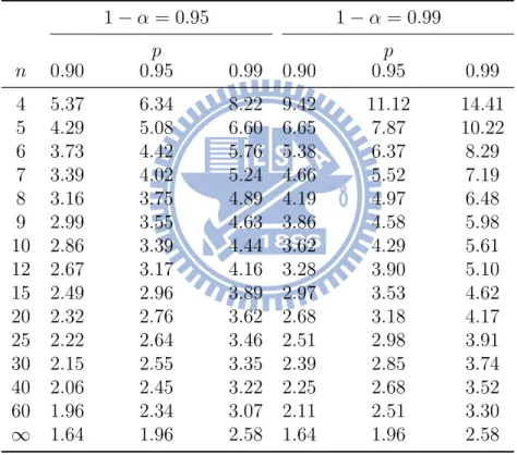
Wald and Wolfowitz (1946) proposed a two-sided β-content, (1− α)-confidence tolerance interval for a normal distribution with the form
(L(X), U (X)) = (¯x− c(1−α;n)s, ¯x + c(1−α;n)s) (5)
where ¯x and s are sample mean and standard deviation of a sample x1, ...xn of size
n, and c(1−α;n) depends on α and sample size n. The c(1−α;n) values are tabulated
in Odeh and Owen (1980) (see Table 1).
For the gamma distribution, let X1, ...., Xnbe a random sample from gamma(α, λ).
Krishnamoorthy, Mathew and Mukherjee (2008) pointed out the transformed sam-ple Y1 = X
1/3
1 , ...., Yn = X
1/3
n can be approximated a normal distribution with an
arbitrary mean µ and arbitrary variance σ2. Then by TI (5), let (L(Y ), U (Y )) be
a two-sided β-content, (1− α)-confidence tolerance interval for this normal distri-bution. Then the gamma(α, λ) distribution approximate tolerance interval with the form
(L(X), U (X)) = (L3(Y ), U3(Y )) (6)
For the data not following the normal distribution but a parametric distribu-tion, we can consider the TI with respect to the distribution (Patel 1986). An
alternative approach is to consider the distribution free TI (Gibbons 1971,1975, Hahn and Meeker 1991). A two-sided β-content, (1− α)-confidence distribution free tolerance interval has the form
(L(X), U (X)) = (X(l), X(u)) (7)
where X(l) and X(u) denote the lth and uth order statistics of the sampled data
x1, ..xn and l and u are chosen symmetrically and as close together as possible
around the integer less than or equal to (n + 1)/2 such that
u∑−l−1 i=0 ( n i ) βi(1− β)n−i ≥ 1 − α.
In the situation without censored data, the above mentioned TIs can be directly used. When the data is twice-censored, directly applying the above TI can not lead to a satisfactory result. Therefore, in this study, we propose approaches based on the above mentioned TIs to construct TI with censored data and show that the proposed algorithm can obtain a desirable result.
3
Methods
3.1
Censored rate method for the normal distribution
For a twice-censored data, a feasible way to construct TI of the sample pop-ulation is to estimate the unknown parameter and then generate a new sample from the distribution based on the estimated parameter value to reconstruct TIs. As mentioned in the introduction section, a widely-used method to estimate the parameter is to adopt the maximum likelihood method. However, it is hard to derive the maximum likelihood approach from the likelihood function when F (x) and S(x) cannot be simplified to forms without involving integrations. In this study, we propose a censored rate approach to estimate the unknown parameter. First, we consider the sampled population is the normal distribution.
Suppose we have a sample Xi = (Zi, δi), i = 1, ..., n from the normal distribution
N (µ, σ2) with the left censored time L and the right censored time U . Suppose
that there are n1, n2 and n3 data corresponding to δi = 1, 2 and 3 respectively. We
call n2/n and n3/n as the right and left censored rates. In the proposed approach,
we use the left and right censored rates to approximate the probabilities P (X > U ) and P (X < L). Therefore, we intend to obtain estimators for µ and σ by solving
P (X < U ) = Φ(U − µ
σ ) = 1− n2/n
P (X < L) = Φ(L− µ
σ ) = n3/n (8)
Let q1 and q2 denote the (1− n2/n) and n3/n quantiles of the standard normal
distribution. Then (8) can be rewritten as
U = µ + q1σ L = µ + q2σ (9) By solving (9), we have: ˆ σ = U− L q1− q2 and ˆµ = (U − q1ˆσ). (10)
Based on the estimators (10), we can generate n3 data greater than U and n2
data less than L from the normal distribution N (ˆµ, ˆσ2). Then based on the new
n2+ n3 data and the n1 uncensored data, we can derive the TIs based on (5) and
(7). If the sample size n = n1 + n2+ n3 is large, we can directly use the n data.
If the sample size n = n1+ n2+ n3 is not large, we can generate more data based
from the normal distribution N (ˆµ, ˆσ2) to derive TIs. The approach is summarized
as the following procedure.
Procedure 1: constructing TIs for a normal distribution with cen-sored data
For a data following a normal distribution N (µ, σ2) with a right censored time
U and a left censored time L, the steps of deriving TIs are listed below.
Step 1. Calculate the estimators (10) of (µ, σ).
Step 2. If the sample size n of the data is large, generate n2 data greater than the
from the normal distribution N (ˆµ, ˆσ) to replace the n2+ n3 censored data. If the
sample size n of the data is small, generate a sample with a larger sample size from the normal distribution N (ˆµ, ˆσ).
Step 3. Base on the n2+n3 data obtained from Step 2 and the n1 uncensored data
to derive tolerance interval (5) and distribution-free tolerance interval(7) when the sample size n is large. Or base on the generated data with a larger sample size to derive tolerance intervals.
3.2
Censored rate approach for general distributions
For a distribution with a density function or probability function f (x|θ), we propose a general procedure based on the censored rate estimation to estimate the unknown parameters, where θ is a vector of unknown parameters. Similarly as for the normal distribution, we use n2/n, and n3/n to estimate Pθ(X ≥ U) and
Pθ(X ≤ L). Since we expect that the probabilities P (X ≥ U|ˆθ) and P (X ≤ L|ˆθ)
are close to n2/n, and n3/n asymptotically. Thus, for an estimator ˆθ, we propose
an error function ε(ˆθ) = (P (X ≤ L|ˆθ) − n3 n ) 2 + (P (X ≥ U|ˆθ) −n2 n ) 2 (11)
to evaluate the estimator ˆθ. An estimator with a smaller error function value is
better than an estimator with a larger error function value.
The method we propose is first to use the n1 uncensored data to derive a
maximum likelihood estimator of θ, say ˆθ(1). Then the second step is to generate
estimator based on the new generate data, say ˆθ(2). Then we repeat the process to derive ˆθ(i), i = 3, ..., m, where m can be chosen as 100. Then we calculate
ε(ˆθ(i)), i = 1, ..., m. Under the error function (11), the ˆθ(i) with the smallest ε(ˆθ(i))
is regarded as the desired estimator. The steps of deriving TIs with censored data for a distribution is give in the following procedure.
Procedure 2: constructing tolerance interval for general distributions with censored data
For data following a distribution with a density function or a probability func-tion f (x|θ) with a right censored time U and a left censored time L, the steps of deriving TIs are listed below.
Step 1. Use n1 uncensored data to derive the maximum likelihood estimators of
θ, say ˆθ(1) and then calculate ε(ˆθ(1)) for the maximum likelihood estimator.
Step 2. Generate n2 and n3 data which are greater than U and less than L
respectively based on the density or probability function f (x, ˆθ(i)).
Step 3. Calculate the maximum likelihood estimator of θ, say ˆθ(i+1), based on the
n1+ n2+ n3 data and calculate ε(ˆθ(i+1)).
Step 4. Repeat Steps 2 and 3 k times to obtain ˆθ(i+1), i = 1, ..., k
Step 5. Find the ˆθ(i)with the smallest ε(ˆθ(i)) value among the (k+1) ε(ˆθ(i)) values.
Step 6. Generate data based on the θ value derived in Step 5. And base on these
4
Simulation
In this section, we conduct a simulation study to evaluate the TIs derived by the procedures presented in Section 3. We use the β−expection criterion to evaluate a TI. That is, we evaluate the performance of a tolerance interval (L(X), U (X)) by its expected coverage proportion, which is defined to be
eθ(L(X), U (X)) = Eθ(F (U (X))− F (L(X))). (12)
It is worth noting that we use the β−expectation criterion to evaluate TIs instead of using the β−content criterion, which is to evaluate the performance of TIs by calculating the coverage probability rθ(L(X), U (X)) = Pθ(F (U (X))−
F (L(X)) > β). The β−content criterion is stricter than β−expectation criterion
because rθ(L(X), U (X)) > 1− α implies eθ(L(X), U (X)) > β if α < 1/2.
In this simulation study, we use the normal distribution and the gamma dis-tribution as examples to show the performance of the proposed methods. First, the coverage probabilities of TIs without censoring case are calculated for different sample sizes. Then we generate data and censor the data greater than a upper cen-sored time U and less than a lower cencen-sored time L. By applying Procedures 1
and 2 to the uncensored data to derive TIs, we calculate the coverage probabilities
of 0.9-content, 0.95 level TIs for different censored rates.
4.1
Normal Distribution
Table 1 presents the coverage proportions of TIs for the case without censored data and the cases for different censored rates for the normal distribution.
Table 1 shows the expected coverage probability with different censored rates:
Table 1: Coverage proportions of 0.9 content, level 1− α = 0.95 TIs (5) and (7) for the standard normal distribution N (0, 1) for different censored rate s
Sample size n 50 100 500 1000 Uncensored TI 0.9426848 0.9341925 0.9179708 0.9115069 (L, U ) = (−1.4, 1), s = 0.239 TI (5) 0.947882 0.93905 0.916313 0.911379 Distribution-free TI (7) 0.956301 0.954294 0.919415 0.914434 (L, U ) = (−0.6, 1), s = 0.433 TI (5) 0.942749 0.929939 0.915095 0.910275 Distribution-free TI (7) 0.955512 0.945512 0.91995 0.913309 (L, U ) = (−0.6, 0.6), s = 0.548 TI (5) 0.939381 0.93231 0.914093 0.914511 Distribution-free TI (7) 0.953178 0.949264 0.920145 0.917852 (L, U ) = (−0.2, 0.6), s = 0.695 TI (5) 0.937867 0.938966 0.907528 0.911114 Distribution-free TI (7) 0.95215 0.952404 0.913157 0.913473 (L, U ) = (0.2, 1), s = 0.737 TI (5) 0.946476 0.929956 0.917268 0.910407 Distribution-free TI (7) 0.956862 0.942909 0.921643 0.913668
0.2 0.3 0.4 0.5 0.6 0.7 0.8 0.88 0.90 0.92 0.94 0.96 Censored rate Co v er age
Figure 1: N(0,1) coverage proportions of TI (5) for sample size n=100 with different censored rate (solid line) and coverage proportions with uncensored case (dashed line) 0.2 0.3 0.4 0.5 0.6 0.7 0.8 0.88 0.90 0.92 0.94 0.96 Censored rate Co v er age
Figure 2: N(0,1) coverage proportions of TI (5) for sample size n=500 with different censored rate (solid line) and coverage proportions with uncensored case (dashed line)
Table 1 shows the coverage proportions of TIs are always greater than the setted
β value 0.9. The coverage proportions tend to the setted β− value 0.9 when the
sample size increases. To achieve a better result for the small sample size case, we generate more data from the distribution based on the estimators (ˆµ, ˆs) and then
based on the data to calculate TIs.
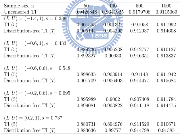
Table 2 shows the coverage proportion with different censored rates using the generated 1000 data:
Table 2: Coverage proportions by regenerated 1000 data of 0.9 content, level 1−α = 0.95 TIs (5) and (7) for the standard normal distribution N (0, 1) for different censored rate s Sample size n 50 100 500 1000 Uncensored TI 0.9426848 0.9341925 0.9179708 0.9115069 (L, U ) = (−1.4, 1), s = 0.239 TI (5) 0.901595 0.901327 0.91058 0.911992 Distribution-free TI (7) 0.905144 0.904295 0.912937 0.914608 (L, U ) = (−0.6, 1), s = 0.433 TI (5) 0.889236 0.906238 0.912777 0.910127 Distribution-free TI (7) 0.892327 0.90933 0.916351 0.913837 (L, U ) = (−0.6, 0.6), s = 0.548 TI (5) 0.898635 0.903914 0.91148 0.911942 Distribution-free TI (7) 0.901709 0.906403 0.914477 0.915684 (L, U ) = (−0.2, 0.6), s = 0.695 TI (5) 0.895989 0.9002 0.907408 0.911784 Distribution-free TI (7) 0.899081 0.903822 0.911118 0.914475 (L, U ) = (0.2, 1), s = 0.737 TI (5) 0.880731 0.894976 0.911529 0.910671 Distribution-free TI (7) 0.883636 0.89777 0.914798 0.91385
0.2 0.3 0.4 0.5 0.6 0.7 0.8 0.88 0.90 0.92 0.94 0.96 Censored rate Co v er age
Figure 3: N(0,1) coverage proportions by regenerated 1000 data of TI (5) for sample size n=100 with different censored rate(solid line) and coverage proportions with uncensored case (dashed line)
0.2 0.3 0.4 0.5 0.6 0.7 0.8 0.88 0.90 0.92 0.94 0.96 Censored rate Co v er age
Figure 4: N(0,1) coverage proportions by regenerated 1000 data of TI(5) for sample size n=500 with different censored rate(solid line) and coverage proportions with uncensored case (dashed line)
From Tables 1-2, it reveals that the sample size n increases, the coverage proportions will much close to 0.9. It means that sample size n increases, then the accuracy of tolerance interval will increase too. For small sample size situation. from Table 2 result, we can use regenerate data method to increase accuracy.
Figures 1-2 show that when the censored rate increases, coverage proportion is still close to uncensored situation. And coverage proportion are higher than 0.9 in Figures 1-4. It reveals that the normal method is a good way to construct the tolerance interval for normal distribution.
4.2
Gamma distribution simulation
Then we consider the gamma distribution case. We generate data form the gamma distribution G(4, 0.05) under different censored times L and U , and then adopt
Procedure 2 with k = 100 to generate data , ˆα and ˆλ. The performance of
Table 3: Coverage proportions of 0.9 content, level 1− α = 0.95 TIs (6) and (7) for the gamma distribution G(4, 0.05) for different censored rate s
sample size n 50 100 500 1000 Uncensored TI 0.9402119 0.9357238 0.916368 0.9105909 (L, U ) = (10, 110), s = 0.203 TI (6) 0.947519 0.934563 0.918274 0.911681 Distribution-free TI (7) 0.958208 0.947696 0.923222 0.914777 (L, U ) = (20, 100), s = 0.284 TI (6) 0.942466 0.937306 0.916717 0.910158 Distribution-free TI (7) 0.948382 0.949671 0.921288 0.912783 (L, U ) = (30, 90), s = 0.408 TI (6) 0.939538 0.93021 0.917118 0.912648 Distribution-free TI (7) 0.947022 0.946774 0.922243 0.915167 (L, U ) = (35, 85), s = 0.487 TI (6) 0.949929 0.934746 0.91729 0.911581 Distribution-free TI (7) 0.961445 0.948354 0.922517 0.915089 (L, U ) = (40, 80), s = 0.576 TI (6) 0.942529 0.935224 0.916078 0.910171 Distribution-free TI (7) 0.953255 0.949475 0.920472 0.912968
0.2 0.3 0.4 0.5 0.6 0.7 0.8 0.88 0.90 0.92 0.94 0.96 Censored rate Co v er age
Figure 5: G(4,0.05) coverage proportions of TI (6) for sample size n=100 with different censored rate (solid line) and coverage proportions with uncensored case (dashed line) 0.2 0.3 0.4 0.5 0.6 0.7 0.8 0.88 0.90 0.92 0.94 0.96 Censored rate Co v er age
Figure 6: G(4,0.05) coverage proportions of TI (6) for sample size n=500 with different censored rate (solid line) and coverage proportions with uncensored case (dashed line)
Table 4: Coverage proportions by regenerate 1000 data of 0.9 content, level 1− α TIs (6) and (7) for the gamma distribution G(4, 0.05) for different censored rate s
sample size n 50 100 500 1000 Uncensored TI 0.9402119 0.9357238 0.916368 0.9105909 (L, U ) = (10, 110), s = 0.203 TI (6) 0.896458 0.907104 0.911554 0.911693 Distribution-free TI (7) 0.899885 0.911698 0.914112 0.914507 (L, U ) = (20, 100), s = 0.284 TI (6) 0.904749 0.914296 0.908947 0.911292 Distribution-free TI (7) 0.907736 0.916863 0.911582 0.915556 (L, U ) = (30, 90), s = 0.408 TI (6) 0.902437 0.904648 0.911802 0.912217 Distribution-free TI (7) 0.905624 0.908264 0.915571 0.916125 (L, U ) = (35, 85), s = 0.487 TI (6) 0.903451 0.902536 0.908789 0.912732 Distribution-free TI (7) 0.906411 0.905598 0.912366 0.91565 (L, U ) = (40, 80), s = 0.576 TI (6) 0.887841 0.909547 0.914453 0.912056 Distribution-free TI (7) 0.892355 0.912906 0.916733 0.915406
0.2 0.3 0.4 0.5 0.6 0.7 0.8 0.88 0.90 0.92 0.94 0.96 Censored rate Co v er age
Figure 7: G(4,0.05) coverage proportions by regenerated 1000 data of TI (6) for sample size n=100 with different censored rate(solid line) and coverage proportions with uncensored case (dashed line)
0.2 0.3 0.4 0.5 0.6 0.7 0.8 0.88 0.90 0.92 0.94 0.96 Censored rate Co v er age
Figure 8: G(4,0.05) coverage proportions by regenerated 1000 data of TI (6) for sample size n=500 with different censored rate(solid line) and coverage proportions with uncensored case (dashed line)
From Tables 3-4, it reveals that the coverage proportions of the tolerance inter-val and distribution-free tolerance interinter-val for the gamma distribution are higher than 0.9. When the sample size increases, the coverage proportion tend to be close to 0.9. As for small sample size situation, we can adopt Procedure 2 to generate more data to improve the estimation.
From Figures 5-8, it reveals that when the censored rate increases, coverage proportion is more far away from the coverage proportions with uncensored rate case. But it still higher than 0.9. It reveals that the general approach method is a good way to construct the tolerance interval for continuous distributions.
If we increase sample size n and iteration time k, the general approach method is more accurate. However, if the iteration time k is too large, it is time consumption. So choose the suitable iteration times (k = 100) can make the coverage more accuracy with shorter simulation time.
5
A real data example
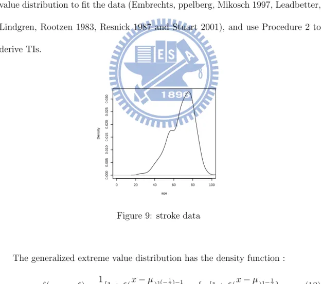
A data set which record the ages at first stroke of 1205 patients from a hospital in Taiwan is used to illustrate the methods. The data is given in the Appendix. Figure 9 shows an approximately density function fitting the 1205 data. The sample mean and standard deviation of the 1205 data are 68.36 and 13.07 respectively. Since it is not symmetric curve and is skewed to the right, we expect it is not a normal distribution. To obtain a better result, we consider using the generalized extreme value distribution to fit the data (Embrechts, ppelberg, Mikosch 1997, Leadbetter, Lindgren, Rootzen 1983, Resnick 1987 and Stuart 2001), and use Procedure 2 to derive TIs. 0 20 40 60 80 100 0.000 0.005 0.010 0.015 0.020 0.025 0.030 age Density
Figure 9: stroke data
The generalized extreme value distribution has the density function :
f (x; µ, σ, ξ) = 1 σ[1 + ξ( x− µ σ )] (−1ξ)−1 exp{−[1 + ξ(x− µ σ )] −1 ξ} (13)
is a scale parameter with σ > 0 and ξ is a shape parameter with −∞ < ξ < ∞. Figures 10 and 11 are two density functions with respect to different parameter values. −2 −1 0 1 2 3 4 5 0.0 0.1 0.2 0.3 0.4 value Density
Figure 10: The density function of the generalized extreme value distribution with
µ = 0, σ = 1, ξ = 0.5 −5 −4 −3 −2 −1 0 1 2 0.0 0.1 0.2 0.3 0.4 value Density
Figure 11: The density function of the generalized extreme value distribution with
Table 5: Coverage proportions for TI (5), distribution-free TI (7) based on the normal distribution and distribution free TI based on the GEV distribution for the stroke data
True T.I (43.74,86.38) Censored time (L, U ) (55,95) (60,90) (65,85) Censored rate 0.171784 0.273858 0.418257 Normal T.I (5) (48.09,89.52) (49.01,89.15) (51.59,88.53) Coverage proportions 0.904564 0.892116 0.860580 Distribution-free Normal T.I (7) (47.58,86.87) (48.16,86.87) (51.44,88.30) Coverage proportions 0.882157 0.878838 0.861410 Distribution-free GEV T.I (7) (41.73,86.87) (40.50,86.87) (43.12,86.22) Coverage proportions 0.921991 0.926971 0.903734
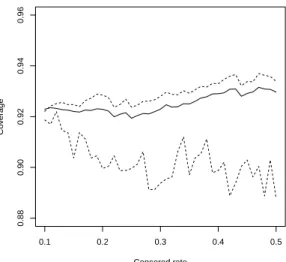
0.1 0.2 0.3 0.4 0.5 0.88 0.90 0.92 0.94 0.96 Censored rate Co v er age
Figure 12: Coverage proportions for stroke of TI (5)(solid line), distribution-free TI (7)(upper dashed line), and GEV distribution-free TI (lower dashed line)
From Table 5 and Figure 12, it reveals that the coverage proportion of GEV distribution-free tolerance interval is much close to 0.9 than tolerance interval and distribution-free tolerance interval based on the normal distribution. And when censored rate increases, the bias of coverage proportion of three tolerance interval increases. The GEV distribution fits the data better than the normal distribution. The reason may be that the data does not follow normal distribution, but we think the uncensored data follow normal distribution.
However, when the censored rate for data increases, the bias of coverage propor-tion increases. Then using normal method to construct tolerance interval is better than GEV method in this example. Therefore, if the censored rate is too large, using normal distribution method will better than GEV distribution method.
References
[1] Cai, T. and Wang, H. (2009). Tolerance Intervals for Discrete Distributions in Exponential Families. Statistica Sinica, 19, 905-923.
[2] Coles, Stuart (2001). An introduction to Statistical modeling of Extreme Val-ues. Springer Statist.
[3] Cummings, J., Zhou, C and Dive, C. (2011). Application of the β-expectation tolerance interval to method validation of the M30 and M65 ELISA cell death biomarker assays. J Chromatogr B Analyt Technol Biomed Life Sci. Apr 15;879(13-14):887-93.
[4] Embrechts,P,Klppelberg,C , and Mikosch,T. (1997) Modelling extremal events for insurance and finance. Springer,Berlin.
[5] Emura, T. and Wang, H. (2010). Approximate Tolerance Limits Under Log-location-scale Regression Models in the Presence of Censoring, Technometrics, 52, 313-323.
[6] Gebizlioglu, O. L. and Yagci, B. (2008). Tolerance intervals for quantiles of bivariate risks and risk measurement. Insurance: Mathematics and Economics 42, 1022-1027.
[7] Gibbons, J. D. (1971), Nonparametric Statistical Inference, New York: McGraw-Hill Book Co.
[8] Gibbons, J. D. (1975), Nonparametric Methods for Quantitative Analysis, New York: Holt, Rinehart, Winston.
[9] Hahn, G.J.(1970b), Statistical intervals for a normal population. Part I. Ta-bles, examples and applications, Journal of Quality Technology 2, 115-125.
[10] Hahn, G. J. and Chandra, R. (1981). Tolerance intervals for Poisson and Binomial variables. J. Quality Tech. 13, 100-110.
[11] Hahn, G. J. and Meeker, W. Q. (1991). Statistical Intervals: A Guide for Practitioners. Wiley Series.
[12] Krishnamoorthy, K and Mathew, T and Mukherjee, S (2008). Normal-Based Methods for a Gamma Distribution: Prediction and Tolerance Intervals and Stress-Strength Reliability. Technometrics, 50, 69-78.
[13] Krishnamoorthy, K. and Mallick, A. and Thomas Mathew, T. (2011) Inference for the Lognormal Mean and Quantiles Based on Samples With Left and Right Type I Censoring, Technometrics, 53, 72-82.
[14] Leadbetter, M.R., Lindgren, G. and Rootzn, H. (1983). Extremes and related properties of random sequences and processes. Springer: New York.
[15] Miller, R. G., Jr. (1981), Simultaneous Statistical Inference (Second Edition), New York: Springer-Verlag.
[16] Odeh, R. E.,and Owen, D. B.(1980), Tables for Normal Tolerance Limits, Sampling Plans, and Screening, New York: Marcel Dekker, Inc.
[17] Patel, J. K. (1986), Tolerance Intervals, a Review, Communication in Statis-tics, Theory and Methods, 15, 2719-2762.
[18] Patilea, V. and Rolin, J.-M. (2006), Product-limit estimators of the survival function with twice censored data. Ann Statist., 34(2),Page 925-938.
[19] Resnick, S.I. (1987). Extreme values, regular variation and point processes. Springer-Verlag, New York.
[20] Shen ,P (2009), Nonparametric Estimators of the Survival Function with Twice Censored Data. Ann Inst Stat Math.1-10.
[21] Wald, A. and Wolfowitz, J. (1946). Tolerance limits for normal distribution. Ann. Math. Statist. 17, 208-215.
[22] Wang, H. (2007). Estimation of the probability of passing the USP dissolution test. J Biopharm Stat, 17, 407-413.
[23] Wang, H. and Tsung, F. (2009) . Tolerance Intervals with Improved Coverage Probabilities for Binomial and Poisson Variables. Technometrics, 51, 25-33.
[24] Zaslavsky, BG. (2007). Calculation of tolerance limits and sample size de-termination for clinical trials with dichotomous outcomes. J Biopharm Stat. ;17(3):481-91.
Table 6: Real data for the 1205 ages at first stoke 46.74 44.32 75.75 78.73 71.64 44.48 77.97 47.23 69.72 85.08 61.33 61.79 75.71 76.86 88.65 66.26 78.2 86.05 56.19 76.46 49.75 82.76 81.97 78.47 78.52 57.07 69.8 66.81 51.67 73.93 36.47 69.11 43.74 47.93 64.81 67.13 54.32 93.66 73.75 55.37 74.42 51.56 78.07 81.36 76.67 76.13 44.1 23.7 70.5 66.22 59.89 74.88 68.32 79.98 80.25 64.84 76.48 52.87 67.75 64.17 73.04 82.78 84.23 71.59 86.38 49.25 61.91 79.88 77.12 77.33 86 74.58 71.53 68.27 50.95 69.83 61.36 87.5 90.81 84.58 75.36 54.92 68.22 81.97 69.88 57.98 55.9 54.92 67.95 62.19 40.15 80.67 85.76 73.49 51.96 79.96 65.33 67.75 73.59 76 88.12 61.58 79.06 61.09 73.7 80.7 80.89 48.25 55.93 56.88 77.57 73.8 82.82 66.05 51.64 57.11 56.14 75.76 77.82 74.93 64.9 42.5 44.75 74.5 79.67 70.81 81.51 48.78 53.11 70.11 78.51 79.87 64.85 86.68 83.65 52.7 62.69 32.33 70.67 65.32 87.08 57.73 75.49 65.81 88.26 53.64 74.12 80.56 60.17 76.83 86.55 75.3 53.99 65 66.37 46.64 40.87 60.18 68.75 75.4 86.75 67.45 68.08 78.14 42.95 74.21 43.38 75.3 85.92 75.29 85.33 91.42 77.25 68.27 56.86 64.66 83.79 70.7 72.7 81.76 64.62 62.33 76.86 85.94 77.1 55.65 72.83 57.04 69.01 85.63 52.96 51.74 69.95 74.79 70.8 63.09 39.47 73.1 68 66.98 31.16 72.05 61.81 65.96 77.96 75.33 79.06 41.23 67.82 71.09 78.56 66.19 88.93 83.47 76.73 74.07 68.96 66.39 75.32 83.31 86.58 70.34 71.2 83.28 64.47 77.93 58.3 48.38 75 47.46 46.41 68.9 75.59 75.65 63.83 81.38 75.94 67.72 89.52 78.59 79.71 84.57 78.23 81.26 51.74 58.92 81.83 56.78 76.35 71.87 81.22 76.5 72.3 76.2 63.85 79.52 53.34 73.26 68.22 76.61 63.19 56.21 64.56 65.54 80.44 61.28 76.89 61.01 107.07 78.38 53.13 85.43 86.39 63.95 51.11 73.08 56.3 66.01 80.07 84.44 49.48 50.02 77.43 39.18 46.98 52.65 44.05 44.47 46.04 80.54 41.43 61.03 68.57 88.31 39.19 73.52 78.6 63.23 65.05 67.2 67.09 58.33 79.82 35.36 58.22 61.98 84.85 93.98 64.79 82.18 83.72 76.87 83.92 47.04 71.03 86.31 55.65 58.2 81.71 79.22 55.97 66.31 49.24 72.93 65.92 77.7 71.04 69.19 95.14 63.22 42.58 82.74 57.2 72.36 59.72 72.1 78.79 67.99 66.65 66.42 76.34 65.21 61.55 53.9 55.9 56.74 79.59 78.65 83.81 61.22 67.52 60.43 69.4 77.84 63.81 75.2 66.45 67.47 55.12 74.22 66.3 69.19 68.1 64.81 84.03 77.35 81.51 58.71 68.34 59.44 75.43 68.32 68.47 62.36 67.37 78.02 27.62 82.3 78.67 83.52 60.65 64.45 72.66 45.62 57.72 74.31 67.26 88.7 58.31 55.47
80.37 67.28 51.17 80.51 77.19 70.56 67.61 53.45 71.54 84.44 67.07 76.38 75.37 56.81 76.45 68.85 83.32 84.13 79.46 56.22 78.61 76.15 75.81 77.18 71.64 88.07 88.08 89.96 76.82 65.31 56.87 71.98 66.77 77.16 72.92 80.84 65.47 63.87 81.44 82.78 78.39 71.59 61.53 73.28 70.7 42.13 68.52 71.68 73.79 70.93 59.12 69.19 59.99 76.98 68.67 70.94 71.61 79.21 74.99 52.82 57.76 66.56 48.24 79.66 79.1 73.64 56.82 84.03 87.4 76.11 72.22 65.73 48.54 65.87 65.71 64.97 82.54 72.8 54.54 75.91 55.5 78.37 78.44 63.21 72.18 79.16 86.62 76.68 61.53 81.91 70.04 76.98 88.77 41.53 60.34 76.27 53.41 53.78 77.58 49.95 54.03 85.63 70.32 70.72 78.54 75.64 77.44 31.86 72.02 62.12 75.45 79.81 81.87 59.56 68.09 59.77 73.71 56.57 57.44 62.63 60.42 80.46 65.23 69.76 53.41 54.1 60.98 80.87 79.61 65.32 38.15 81.32 82.83 81.02 80.17 55.91 64.85 72.75 78.35 83.15 75.54 71.38 68.15 72.43 68.24 76.86 67.09 86.94 72.17 58.5 68.69 64.86 64.42 39.1 73 46.83 75.45 77.47 81.41 73.11 64.04 72.46 88.58 82.43 58.55 83.79 80.58 79.93 72.03 74.63 60.16 34.64 72.3 54.13 72.63 68.62 80.22 44.65 79.48 77.72 49.16 71.34 67.08 39.68 71.84 72.05 75.7 54.12 65.24 68.62 82.43 37.46 78.41 69.36 82.16 51.56 85.78 73.95 62.58 56.42 74.72 74.19 66.5 55.95 66.32 82.25 48.53 68.5 80.08 72.47 38.76 56.96 66.5 59.44 71.98 74.27 27 91.93 71.31 62.83 63.67 58.34 78.53 68.65 89.59 72.27 68.85 43.72 69.05 48.38 65.28 50.87 76.25 73.4 77.53 74.03 51.41 71.7 93.84 53.64 78.42 67.3 73.08 84.31 56.58 70.04 64.84 81.55 76.22 70.54 76.42 76.67 69.37 71.08 53.15 76.32 57.71 43.07 59.18 76.02 78.04 48.92 58.92 73.78 62.78 69.55 51.48 64.82 56.33 27.13 55.61 76.81 86.95 62.9 46.5 75.71 70.82 76.13 68.82 45.25 70.45 77.14 80.72 66.64 62.41 80.97 73.8 80.12 55.13 58.73 54.14 82.35 72.96 42.79 64.94 39.04 75.83 74.47 62.37 61.98 75.45 67.42 55.11 68.54 64.65 53.08 72.38 74.59 79.4 56.38 65.52 64.15 70.99 95 58.66 57.88 63.62 87.07 71.64 67.42 79.39 46.02 49.67 73.2 66.98 61.05 25.74 55.68 76.19 79.07 82.54 91.76 66.21 82.02 75.2 83 76.73 81.44 79.94 78.42 79.92 73.95 57.03 72.91 61.98 61.5 93.75 73.84 83.32 63.72 79.46 67.54 52.12 75.36 69.78 80.86 85.57 49.92 54.06 80.81 68.08 78.85 76.04 80.51 74.93 58.32 64.04 82.62 74.35 78.89 76.88 57.58 36.59 86.13 87.43 73.97 89 75.79 79.15 89.08 73.8 86.56 80.04 67.15 78.21 39.82 77.14 82.8 79.47 52.61 71.93 55.56 76.42 77.72 80.32 80.24 84.29 71.45 78.54 52.17
71.36 37.14 47.79 45.17 57.82 84.32 58.83 78.99 72.7 82.86 42.88 83.69 82.56 78.38 86.88 80.57 87.09 86.01 62.89 77.05 72.72 75.51 75.18 84.33 67.75 80.76 56.13 65.25 74.25 81.34 35.33 86.39 44.63 71.32 78.58 65.78 63.27 70.45 61.8 66.35 67.2 53.41 85.28 81.17 85.65 73.71 69.58 72.25 60.02 59.79 91.99 65.28 54.55 54.09 66.56 86.22 73.86 77.22 69.79 58.97 46.02 65.07 75.06 76.8 88.22 88.53 49.16 80.12 84.56 63.24 70.01 90.02 65.36 72.88 51.6 72.13 70.36 82.62 52.43 71.1 46.55 78.6 23.8 67.22 61.06 39.3 73.76 70.91 56.96 73.65 76.21 82.39 57.33 50.82 57.89 73.99 49.68 72.65 72.71 47.13 66.3 79.44 54.04 69.3 32.32 88.15 55.94 56.32 84.49 76.36 33.17 51.99 81.1 50.21 69.1 64.59 108.22 59.31 76.35 82.18 53.5 83.65 68.49 66.45 45.72 73.28 72.02 75.67 69.44 64.75 84.9 70.97 71.38 54.69 58.73 44.9 60.88 62.57 55.35 67.26 70.54 67.38 79.33 63.68 47.79 79.9 72.9 54.21 51.86 82.21 38.38 47.33 82.03 68.52 46.38 43.33 69.25 54.75 53.4 81.62 43.65 69.65 76.45 75.97 65.91 47.85 50.01 48.88 60.2 68.34 51.7 83.68 71.57 50.82 77.84 69.73 100.36 71.9 48.62 55.75 83.23 59.01 67.56 69.48 83.61 70.43 74.18 77.14 49.27 81.27 80.57 70.58 56.95 84.32 51.4 92.25 70.97 81.69 59.42 77.98 66.53 50.46 61.96 39.75 80.69 77.8 72.95 55.44 74.53 54.21 68.07 48.43 78.63 54.73 88.15 49.2 59.47 52.88 65.92 61.48 61.65 64.61 54.14 67.71 37.63 66.47 77.99 78.43 62 67.75 80.98 76.75 40.89 70.09 53.36 81.27 60.48 80.36 69.65 89.13 86.05 54.64 83.77 67.84 84.93 54.19 55.44 74.75 38.22 78 73.45 71 41.98 72.87 84.79 45.16 85.88 71.28 73.16 48.7 68.62 69.76 71.49 79.31 42.15 81.78 60.69 52.67 64.52 65.87 72.89 81.42 58.24 71.5 72.17 76.17 70.76 73.43 73.02 76.59 69.91 71.18 86.67 78.14 77.02 76.56 69.56 59.61 88.16 70.94 65.49 56.06 74.81 71.48 43.68 65.39 76.33 78.97 85.32 74.48 57.15 82.19 71.49 75.78 74.13 72 65.47 93.92 69.16 66 73.26 92.8 59.42 72.91 57.72 43.29 71.65 58.14 65.72 61.74 80.18 56.56 60.17 57.34 74.05 86.89 75.3 81.84 84.97 48.37 75.06 56.85 76.12 80.65 56.03 60.48 61.67 77 77.12 35.61 53.66 76.41 85.86 81.07 66.48 76.94 77.01 69.75 37.67 76.02 62.89 56.01 84.92 54.76 57.99 48.75 79.55 87.57 60.18 73.45 73.55 75.39 54.6 40.85 83.95 69.56 61.19 50.35 55.33 50.26 61.85 85.22 84.49 70.26 77.79 60.89 86.25 42.29 65.98 78.8 68.57 70.85 53.04 67.56 56.89 88.19 69.48 81.38 78.07 78.79 77.79 76.97 55.05 80.62 40.18 67.72 74.48 91.24 64.22 68.63 43.59 81.52 61.19 52.63 65.32 83.37 58.28 54.57 67.82 66.22 57.96 70.39 49.95 80.41 71.61
Table 7: The c(p;n) for two-sided tolerance interval described by a normal distribu-tion 1− α = 0.95 1− α = 0.99 p p n 0.90 0.95 0.99 0.90 0.95 0.99 4 5.37 6.34 8.22 9.42 11.12 14.41 5 4.29 5.08 6.60 6.65 7.87 10.22 6 3.73 4.42 5.76 5.38 6.37 8.29 7 3.39 4.02 5.24 4.66 5.52 7.19 8 3.16 3.75 4.89 4.19 4.97 6.48 9 2.99 3.55 4.63 3.86 4.58 5.98 10 2.86 3.39 4.44 3.62 4.29 5.61 12 2.67 3.17 4.16 3.28 3.90 5.10 15 2.49 2.96 3.89 2.97 3.53 4.62 20 2.32 2.76 3.62 2.68 3.18 4.17 25 2.22 2.64 3.46 2.51 2.98 3.91 30 2.15 2.55 3.35 2.39 2.85 3.74 40 2.06 2.45 3.22 2.25 2.68 3.52 60 1.96 2.34 3.07 2.11 2.51 3.30 ∞ 1.64 1.96 2.58 1.64 1.96 2.58
Table 8: The number v for two-sided distribution-free tolerance interval contains at least 100p% of the Sampled Population with 100(1− α)% Confidence
p = 0.90 p = 0.95 p = 0.99 1− α 1− α 1− α n 0.90 0.95 0.99 0.90 0.95 0.99 0.90 0.95 0.99 10 1 1 1 1 1 1 1 1 1 0.6513 0.6513 0.6513 0.4013 0.4013 0.4013 0.0956 0.0956 0.0956 15 1 1 1 1 1 1 1 1 1 0.7941 0.7941 0.7941 0.5367 0.5367 0.5367 0.1399 0.1399 0.1399 20 1 1 1 1 1 1 1 1 1 0.8784 0.8784 0.8784 0.6415 0.6415 0.6415 0.1821 0.1821 0.1821 25 1 1 1 1 1 1 1 1 1 0.9282 0.9282 0.9282 0.7226 0.7226 0.7226 0.2222 0.2222 0.2222 30 1 1 1 1 1 1 1 1 1 0.9576 0.9576 0.9576 0.7854 0.7854 0.7854 0.2603 0.2603 0.2603 40 2 1 1 1 1 1 1 1 1 0.9195 0.9852 0.9852 0.8715 0.8715 0.8715 0.3310 0.3310 0.3310 50 2 2 1 1 1 1 1 1 1 0.9662 0.9662 0.9948 0.9231 0.9231 0.9231 0.3950 0.3950 0.3950 60 3 2 1 1 1 1 1 1 1 0.9470 0.9862 0.9982 0.9539 0.9539 0.9539 0.4528 0.4528 0.4528 80 5 4 2 2 1 1 1 1 1 0.9120 0.9647 0.9978 0.9139 0.9835 0.9836 0.5525 0.5525 0.5525 100 6 5 4 2 2 1 1 1 1 0.9424 0.9763 0.9922 0.9629 0.9629 0.9941 0.6340 0.6340 0.6340 200 15 13 11 6 5 4 1 1 1 0.9071 0.9680 0.9919 0.9377 0.9736 0.9910 0.8660 0.8660 0.8660 300 23 22 19 10 9 7 1 1 1 0.9301 0.9542 0.9903 0.9350 0.9659 0.9934 0.9510 0.9510 0.9510 400 32 30 27 15 13 11 2 1 1 0.9254 0.9643 0.9908 0.9010 0.9645 0.9906 0.9095 0.9820 0.9820 500 41 39 35 19 17 14 2 2 1 0.9249 0.9607 0.9921 0.9135 0.9657 0.9945 0.9602 0.9602 0.9934 600 51 48 44 23 21 18 3 2 1 0.9043 0.9591 0.9901 0.9247 0.9680 0.9938 0.9389 0.9830 0.9976 800 69 66 61 32 30 26 5 4 2 0.9146 0.9593 0.9912 0.9199 0.9606 0.9935 0.9015 0.9583 0.9971 1000 88 85 79 41 39 35 6 5 3 0.9801 0.9515 0.9901 0.9194 0.966 0.9907 0.9339 0.9713 0.9973