國
立
交
通
大
學
統計學研究所
碩
士
論
文
藥物開發之二元滿足點 Phase II/III 調適性無
縫設計
An Adaptive Seamless Phase II/III Design in Drug Development
for Binary Endpoints
研 究 生:張敏琪
指導教授:蕭金福 教授
藥物開發之二元滿足點 Phase II/III 調適性無縫設計
An Adaptive Seamless Phase II/III Design in Drug Development
for Binary Endpoints
研 究 生:張敏琪 Student:Min-Chi Chang
指導教授:蕭金福 Advisor:Chin-Fu Hsiao
國 立 交 通 大 學
統計學研究所
碩 士 論 文
A ThesisSubmitted to Institute of Statistics College of Science
National Chiao Tung University in partial Fulfillment of the Requirements
for the Degree of Master
in Statistics June 2010
藥物開發之二元滿足點 Phase II/III 調適性無縫設計
研究生:張敏琪 指導教授:蕭金福 博士
國立交通大學統計學研究所碩士班
中文摘要
近幾十年來,對於製藥發展來說,如何設計一個臨床試驗、分析其數據,以 及評估藥物的效益已成為一門重要課題。成功開發新藥物的價格急劇上升,而且 在發展過程中有超過一半的時間和費用被使用於臨床試驗中,因此,臨床試驗不 僅費時且費用昂貴。儘管有許多候選藥物,但研究、開發新藥物的成功率卻是令 人失望的。因此,迫切需要發展一種快速、經濟且適當的方法以減少藥物發展的 時間與花費。此研究中,針對二元滿足點的臨床試驗,提出了一個 phase II/III 的調適性無縫設計。在 phase II 試驗中,一試驗藥物的多種劑量皆與一對照組做 比較,以便評估新藥的療效。若有一些劑量在此階段被證實是有效的,或是所有 的劑量皆無效,則試驗將提早結束;否則這些劑量組被允許進入 phase III 試驗。 在最終資料分析時,我們使用兩階段的數據,如此一來,可節省更多的病患資料 及提供更多藥物安全性的訊息。因此,節省資源和成本,縮短臨床試驗發展時間 是有可能的。 關鍵字:調適性設計、Phase II/III 設計、臨床試驗An Adaptive Seamless Phase II/III Design in Drug Development for
Binary Endpoints
Student: Min-Chi Chang Advisor: Dr. Chin-Fu Hsiao
Institute of Statistics National Chiao Tung University
Abstract
In recent decades, how to design a clinical trial, to analyze the data, and to evaluate the benefit of drugs as a whole becomes an important course for pharmaceutical development. The price of successfully developing new drugs has risen steeply, and more than half of the time and expense in the development process are spent in clinical trials. Thus the process of clinical trials is not only time-consuming but also costly. However, the success rate of researching and developing new drugs is disappointing even though there are many potential candidates. As a result, there is an urgent need to conduct a clinical trial by a quick, economical and suitable approach. In this paper, an adaptive phase II/III design which is based on a dichotomous endpoint is proposed in order to reduce the cost and time of developing a drug. At the first stage (the phase II stage), we provide the contrasts between several doses of a test drug and a concurrent control group so that we can evaluate the efficacy of doses of the test drug over the control group. The trial will be stopped early because of efficacy of some doses or futility of all doses. Otherwise, the promising dose groups are permitted to enter the next stage (the phase III stage). We perform the final analysis with the cumulative data from both the phase II stage and the phase III stage so that it can save dataform patients and provide more information about safety. Therefore, considerably saving resource and cost and shortening the duration of clinical trials may be possible.
誌謝
首先,要感謝的是指導教授蕭金福老師,在老師的引導及用心的教導下,讓 原本對藥物試驗一竅不通的我完成了一篇關於臨床試驗的論文;在這段期間內, 當我遇到困惑時,蕭老師總是不厭其煩地替我解答,著實讓我學習到許多臨床試 驗或統計相關的知識。另外,亦要謝謝口試委員黃郁芬老師、鄒小蕙老師以及陳 鄰安老師的建議,讓這篇論文更加完善。 感謝交大統計所老師們的指導,讓我能夠於 2010 年完成碩士學位;在學的 兩年內,不僅從老師們身上學到了統計專業知識,心靈上亦茁壯成長。很開心有 各位同學、朋友的陪伴,讓我在就讀研究所的期間,留下了許多深刻的回憶。最 後,謝謝家人的支持讓我無後顧之憂地繼續修讀碩士學位,謝謝你們溫暖的陪伴。 敏琪 謹誌於 國立交通大學統計學研究所 中華民國九十九年六月Content
中文摘要 .………...
i
Abstract ...……… ii
誌謝 ………...….
iii
Content …………...………. iv
1. Introduction ………
1
2. The Design ……….………
5
3. Results ………
11
4. Conclusion and Discussion ………
14
Tables ………..………
17
Figures ……….………
25
Appendix ……….………
29
1. Introduction
According to the Economist (2002), the cost of developing a drug from screening of candidates to regulatory approval for commercial marketing is between $800 million and $1 billion in the United States (US). It takes more than 12 years on the average; however, more than half of the duration is spent in human experimentation. Hence pharmaceutical development is a costly and time-consuming endeavor. In spite of a better understanding of disease etiology and promotion in medical technology, the success rate of drug development is disappointing. Because only 1 out of 10,000 candidates screened in the laboratory will survive to market launch, and more than 60% of the potential candidates that enter clinical trials fail. One of the many probable reasons is that the method used in the past decades is no longer working for the new century. Consequently, there is an urgent need to develop new concept and methodology to increase the success rate and reduce the cost of money and time in order to take a great benefit to patients and pharmaceutical factories.
Recently, an adaptive seamless phase II/III design has been considered as one possible way to shorten the drug development time and thus reduce patient exposure needed to discover, develop, and demonstrate the benefits of a new drug [1]. It is planed as a design which can be modified during the course of the clinical trial. And it merges several trials that would carry out separately into a single trial. The main goal of the learning stage (the phase II stage) is to figure out whether the drugs has any significant biologic effect, whereas the goal of the confirming stage (the phase III stage) is to assess the efficacy of the treatment selected from the last stage. In an adaptive seamless phase II/III design, we combine the phase II stage which includes several treatments and concurrent control group and the phase III stage into a single trial, and gather data from the two stages to perform the final analysis. The patients in
the learning stage would be monitored continuously until the final analysis, so such a design can help us to get more information of long-term safety effects.
Simon (1989) has proposed an optimal two-stage design which includes one new regimen and one standard therapy for binary endpoints. It minimizes the expected sample size subject to constraints of the type I and II errors if the new regimen has low activity. Tsou et al. (2008) presented a two-stage design for drug screening trials based on continuous endpoints. In addition to minimizing the expected sample size, they also showed the results of the method that minimizes the maximum sample size. A two-stage design for survival endpoint, proposed by Schaid et al. (1990), enables the screening, at the first stage, of several experiments and allows promising treatments to enter the next stage. Their procedure is to minimize the number of patients expected to be accrued to the new regimens which do not offer a survival benefit over the standard regimen, subject to the constraints of alpha-error and power. In addition, they permit a stopping rule when no new regimens show a minimum pre-indicated advantage or some new regimen manifests an overwhelming benefit over the standard regimen. Scher and Heller (2002) made an experiment design developed by Schaid et al. about castrate metastatic prostate cancer and concluded that this design is valuable in some situations. A two-stage adaptive design combining phase II and III trials was proposed by Liu and Pledger (2005). In the first stage, short-term safety and efficacy are examined, and the trial continues to the next stage with the doses that do not lack efficacy or cause safety concerns. Patients from both the first and second stages are evaluated by a long-term clinical endpoint. At the final analysis, pairwise statistics for two stages are combined to establish dose-response
the second stage need not be specified in advance to maintain the validity of the trial. Kelly et al. (2005) developed a flexible design that uses adaptive group sequential methodology to monitor an efficient score statistic. Since it is based upon the scores, this method can be applied to binary, ordinal, failure time, or normally distributed outcomes. This approach can have any number of stages, starts with any number of treatments, and allows any number of these to the next stage. Maca et al. (2006) have introduced the general concept of adaptive designs, described the current statistical methodologies that relate to adaptive seamless designs and also discussed the decision process involved with seamless designs.
In this paper, we propose an adaptive seamless phase II/III design based on dichotomous data with controlling overall type I and II error rates. In the learning stage, we employ a randomized parallel design with various doses of a test drug and a concurrent control group for describing the relationship of the dose and response, and then select promising doses for the confirmatory stage. New patients are recruited randomly to the selected doses and control group in the confirmatory stage. At the final analysis, tests are performed based on the cumulative data to identify the efficacy of doses. With the pre-controlled error rates, the sample size per group in each stage and the critical values can be determined by minimizing the expected total sample size under the hypothesis that there is no discrepancy between the dose group and the control group. Moreover, this design permits early termination of accrual of those doses which do not demonstrate a minimum advantage over the control group which is pre-specified by the investigators. We also stop the trial early if some dose shows a substantial advantage over the control group. In this way, shortening the total duration and cutting down the valuable cost and resource of drug development are possible. This adaptive phase II/III design will be conducted with the same study
population under the same primary endpoint, evaluation criteria, and the same protocol. The detail and formula of the trial design is described in Section 2. The numerical result of sample sizes, critical values and simulation study are showed in Section 3. Discussion and final remarks are mentioned in Section 4.
2. The Design
We propose a phase II/III adaptive design for testing a test drug product against a control group based on dichotomous response endpoints. At the phase II stage, we compare several doses for the test drug over the control group simultaneously. If there exists dose groups for the test drug showing promising results, then the selected dose groups as well as the control group will continue accrual to the phase III stage. That is, new patients will be recruited and randomized to receive either the selected doses of the test drug or to the control group. The final analysis includes the data of the selected doses and control groups from both the phase II and phase III stages.
Let K be the number of doses for the test drug at the phase II stage. Let n2 be the number of patients assigned to each of the K doses and the control group. Let
II i
X be the total number of response observed from the n2 patients for the ith group at the phase II stage respectively, i0 ,1 ,2,,K. Here i0 indicates the control group. Let r be the response rate for the ii th group. It follows that X is distributed iII as a binomial distribution B
n2,ri
, where B represents a binomial distribution. It is desired to test the following hypothesis:H0:ri r0 0 vs. HA:ri r0 0, i=1,…, K. (1)
Let rˆ be the estimate of iII r at the phase II stage. Then i
2 ˆ n X r II i II i , . , , 2 , 1 , 0 K
i We can compare the ithdose group with the control group by the statistic II II i II i r r T ˆ ˆ0 .
clinical requirement pre-specified by investigators, it indicates that none of the doses of the test drug displays a promising result and thus the trial will cease early for futility. If some of the observed values of T are greater than iII C2, then it says that there exists at least one dose of the test drug to have overwhelming advantage, and the trial will stop early for efficacy. Otherwise, the accrual of another n patients for 3 each group will continue to the phase III stage for the control group and dose groups for which C1TiII C2.
At the phase III stage, let X be the number of response observed from the iIII
3
n patients in each group. Again, let III i
rˆ be the estimate of r at the phase III stage. i
It follows that 3 2 ˆ n n X X rIII iII iIII i
, for some i which C1TiII C2 and i =0, and
III i II
i X
X is distributed as abinomial distribution B
n2n3,ri
. Let . ˆ ˆiIII 0III III i r r T At the final stage, we can declare that the ith dose is confirmed to be superior to the control group if T >CiIII 3.
Since every dose group for the test drug is compared to the control group, we use the Bonferroni method for adjusting the overall type I error. Let be the pairwise type I error for each comparison. Consequently, K is the overall type I error. Also let be the pairwise type II error. Based on our design, the probability of “accepting” the ith dose group can be written as
(2) , , ; , , ; , , ; Pr Pr Pr , , , , 2 2 2 1 2 3 3 3 2 2 2 2 2 2 2 1 2 , min 1 1 3 0 2 0 1 2 0 , min 1 0 3 3 2 0 0 0 2 2 0 3 2 1 3 2 0
n C n C n x n x C n n y i i n C n x i n C n C n x II II i III II III i II i II II i II II i i n r r y p n r r x p n r r x p x X X C n n X X X X x X X C n X X C C C n ,n ,r r where
t max
nZnt
, and
1 1 1 1 1 , , ; 0 0 , min , 0 max 0 0 0 0 k k i i x n n x k x n i i r r r r x k n k n r r r r n r r x p
,for nxn. Consequently, under the null hypothesis, the pairwise type I error rate and the pairwise power can be expressed as
r0,r0,n2,n3,C1,C2,C3
(3) and1
ri,r0,n2,n3,C1,C2,C3
(4) respectively.If the sample sizes for both stages are large enough, the equation (2) can be rewritten as
, ,
, ,
. 2 , , exp 2 1 , , , , 1 ˆ ˆ ˆ ˆ Pr ˆ ˆ ˆ ˆ Pr , , , , 3 0 0 3 2 3 0 3 3 2 3 , , , , 2 2 0 0 2 0 0 2 0 2 0 3 0 0 2 0 3 2 1 3 2 0 2 0 2 2 0 1 2 1 dt n r r r r n n t n r r n n n C n r r r r t n r r r r n r r C dt t r r C r r t r r g C r r C C C n ,n ,r r i i i n r r C n r r C i i i i i C C II II i III III i II II i II II i i i i
where (.)g represents the probability density function of rˆiII rˆ0II,
ri,r0,n
denotes
n r r r ri 1 i 0 1 0distribution function.
By the previous assumption, the expected total sample size EN under the null hypothesis that ri r0 0 for all K comparisons can be calculated as follows.
1
1
(5) 1 1 1 EN 1 3 2 1 2 3 0 2
K j j K j j p n j n K p n K n j p n Kwhere p is the probability of stopping accrual at the phase II stage and 0 p j
j1,2,,K
is the probability that the accruals for j of the dose groups and the control group are continued to the phase III stage. Note that the equality of the two terms above is due to
K j j p p 1
0 1. To derive p and 0 p , let j
, ,
ˆ ˆ , , ˆ ˆ , , ˆ ˆ 2 0 0 2 0 2 0 2 2 0 1 0 1 2 1 n r r r r n r r r r n r r r r X X X K II II K II II II II K .Under the null hypothesis that ri r0 0, we can derive that
,
, ~ ) ,..., , (X1 X2 XK T NK where NK
,
represents the multivariate normal distribution with mean matrix μ and variance-covariance matrix Σ. Here
T 0 ,..., 0 , 0 , and 1 1 1 2 1 2 1 1 The derivation of the distribution of (X1,X2,...,XK)T is given in the appendix. Consequently, by the previous assumption and Gupta (1963), we can obtain
r r n x x dx C x n r r C x n r r C j K dx dx x x x f j K p j K j K K j n r r C n r r C n r r C n r r C j K n r r C n r r C j 2 2 1 exp 1 , , 1 , , 1 , , , , , 2 2 0 0 1 2 0 0 1 2 0 0 2 1 2 1 , , , , , , , , , , , , 0 0 2 2 2 0 0 1 2 0 0 2 2 0 0 1 2 0 0 1 2 0 0 1
and
, 2 2 1 exp 1 , , 1 2 2 1 exp 1 , , , , , 1 , , , 2 2 0 0 2 2 2 0 0 1 , , 1 2 1 , , , , 1 2 1 , , 0 2 0 0 2 2 0 0 2 2 0 0 1 2 0 0 1
dx x x n r r C dx x x n r r C dx dx x x x f dx dx x x x f p K K n r r C K K n r r C n r r C K K n r r C where is the correlation coefficient of X and i X , j i , and j f
x1,x2,,xK
is K-dimensional normal density with mean and variance-covariance matrix , i.e.,
2 . 1 exp 2 1 2 1 exp 2 1 , , , 1 2 1 2 1 2 1 2 2 1 X X X X x x x f T K T K K In our design, C1 should be pre-specified.
3 2 0 3 , ,r n n r C i is chosen to be
1 1as though it was the critical value of a one-stage design. For specified values of the treatment effect i ri r0, r0, α, β and C1, we determine n2, n3, C2 and C3 to satisfy the two constraints of type I and II error rates (3) and (4), and to minimize the expected total sample size (5) when ri r0 0. We use a C++ program
with use of the IMSL package for determination of sample sizes and critical values for the phase II/III designs.
3. Results
We are at the position to give some examples for the demonstration of our proposed design. Tables 1-6 illustrate the seamless adaptive phase II/III designs for several combinations of parameters with K 1 , K 2 and K 3 ,
K,
0.05,0.2
, i 0.15, 20i 0. ,C10, and C1 0.05. The tabulated results include the critical value C2 for the observed value T that would permit iII early stopping at the phase II stage due to the treatment efficacy, the critical value C 3 for the observed value T that would not reject the treatment at the phase III stage, iIII the sample size n2 required at the phase II stage per group , the sample size n 3 required at the phase III stage per group, the expected total sample size EN when there is no difference of efficacy between the dose groups and the control group, the sample sizes n2 and n required per group for traditional phase II and phase III 3 designs which are evaluated by
2 2 3 2 1 2 i r r Z Z n n where 2 0 r r r i and
11Z , and the ratio of the maximum total sample size required for the phase II/III design versus the maximum total sample size required for the traditional phase II and phase III designs.
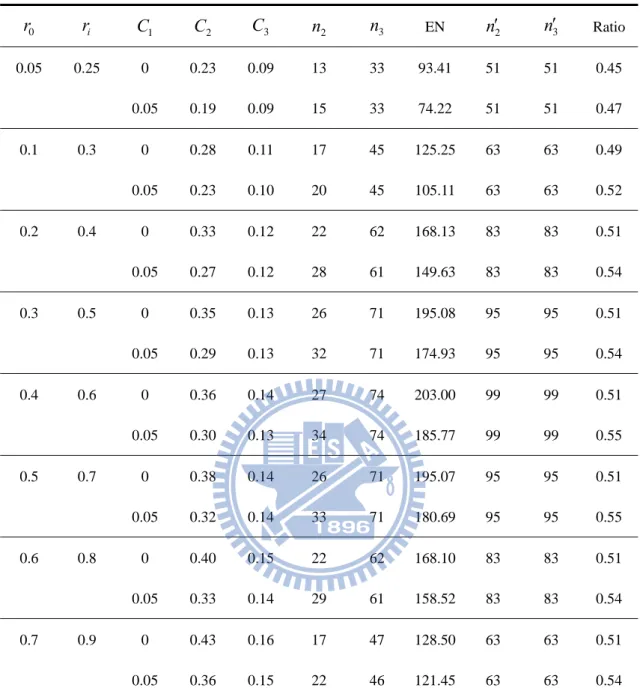
For instance, the first row in Table 3 shows the results corresponding to
K,
0.05,0.2
, 20ri r0 0. , K 2, and C10. With r0 0.05, we enroll 13 patients for each group (that is, 39 patients in total) at the phase II stage. When the trial of the phase II stage is completed, if the observed values of T ’s are all less than iIIterminated for futility. The trial might be stopped as well if some observed value
II i
T is greater than 0.23, interpreted as an indication of overwhelming efficacy of the
dose of the new drug. Otherwise, we need to recruit extra 33 patients for the phase III stage for both the control group and dose groups which 0TiII 0.23. At the final stage, the calculation of the observed value T is based on the accumulated data of iIII
3
2 n
n patients from both phase II and phase III stages. If the observed value III i
T is
less than 0.09, we conclude that there is no difference between the dose groups and the control group. On the contrary, we say that the new drug is more effective than the control group if the observed value T exceeds 0.09. For this design, the expected iIII total sample size is 93.41. The ratio of the maximum total sample size required for the phase II/III design versus the maximum total sample size required for the traditional phase II and phase III designs is 0.45. In other words, the maximum of total sample size required for the phase II/III design can be reduced by around 55% compared with the maximum of total sample size required for the traditional phase II and phase III designs.
It can also be observed that if the difference between the treatment group and the control group increases, both the sample size required for each stage and EN decrease. This makes sense since the larger the treatment effect, the smaller the sample size required. Another feature can be observed is that the required sample sizes per group for each stage increases as C increases. However, as C1 1 increases, both C2 and the expected total sample size decrease. This makes intuitive sense. As C increases, we 1
larger sample size required for each stage. Nevertheless, larger C will cause that the 1 ineffective doses will be quickly eliminated during the phase II stage. Consequently, the probability of early termination for futility at the phase II stage will be increased, and the expected total sample size will be thus reduced.
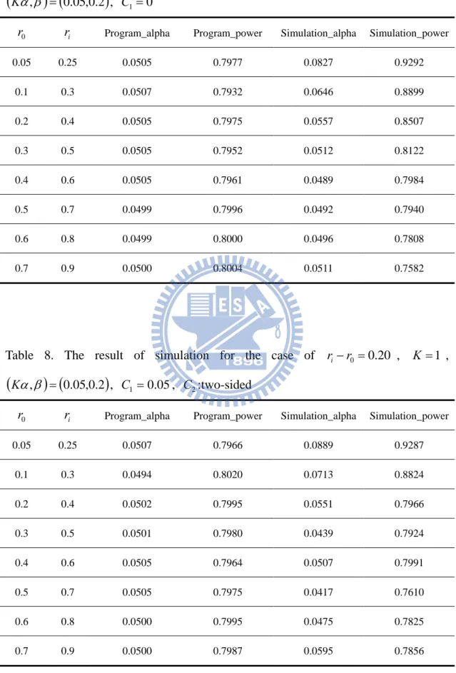
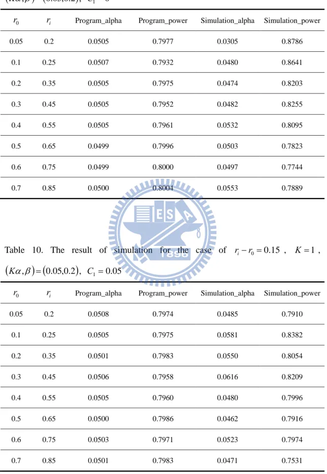
We conduct a simulation study to compare the proposed adaptive phase II/III design with the traditional phase II and phase III designs in terms of success rates. Table 7 and Table 8 display the simulation result for the case of ri r0 0.20 and
0
1
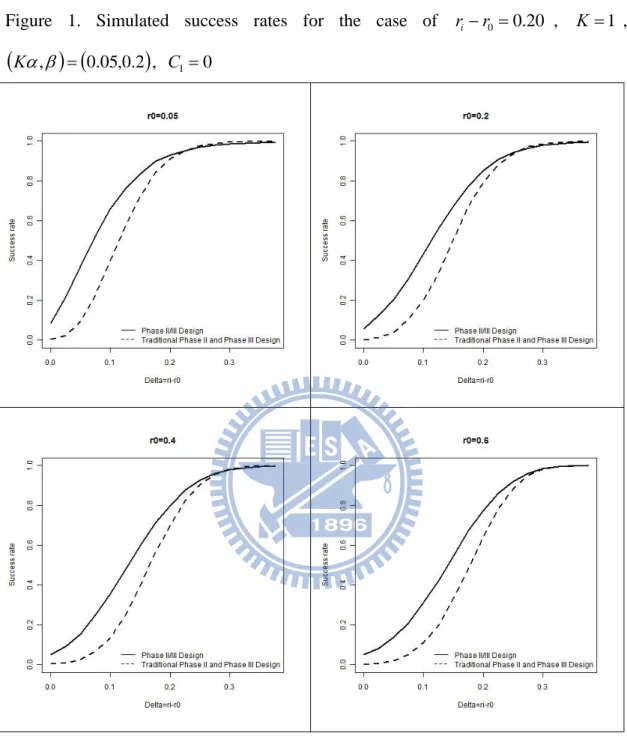
C ,C1 0.05 respectively. Table 9 and Table 10 show the simulation result for the case of ri r0 0.15 and C10,C1 0.05 respectively. From these tables, it should be noted that if the sample size required for each group of phase II stage is less than 30, there exists discrepancy between the results of our program and the simulation due to the Normal approximation. Figure 1 demonstrates the simulation results for the case of ri r0 0.20, K 1,
K,
0.05,0.2
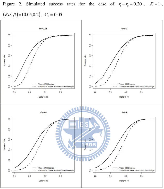
, C10, with various values of r0. Given r0 0.6, we can derive C2 0.37, C3 0.14, n2 20and 49n3 . The power is evaluated for the treatment effect increasing from 0 to i 0.375, by 0.025. The success rate of each was obtained as the proportion of i number of successes from 10,000 replicates. From this graph, the proposed phase II/III design reaches the desired power 0.8 at i 0.2 which is larger than the traditional design. It can be seen from Figure 1 that in most cases, the proposed phase II/III design performs better than the traditional method. Figures 2-4 display the simulation results under other specifications, and similar conclusions can be made.
4. Conclusion and Discussion
In this paper, we propose a seamless adaptive phase II/III design based on binary endpoints for evaluating the efficacy of drugs. One intriguing feature for such designs is the reduction in development time. Since the phase II and phase III trials are combined into a single trial, there will be no lead time between the phase II and phase III clinical developments. Also the data collected from the phase II stage will also be included in the analysis of the phase III stage, and thus the sample size reduction is possible.
As we mentioned, the success rate of drug development has been declined drastically in recent years. Some possible reasons may be that the patient populations recruited for the phase II and phase III trials are different, and also schemes used at the phase II and phase III trials are different. However, in our design, the phase II and phase III trials are conducted in the same protocol with the same inclusion/exclusion criteria, the same study design, the same control group, the same methods for evaluation, and the same efficacy/safety endpoints, the above issues concerning the traditional clinical development can therefore be avoided.
The selection of C1 may be another important issue. As we know, larger value of C1 will produce higher probability of early stopping, and thus reduce the expected
total sample sizes. On the other hand, larger value of C1 can also increase the success probability of the phase III stage for the clinical development. However, most of all, the determination of C1 should meet the minimal clinically meaningful requirement that an investigator would need to observe before continuing accrual onto the phase
In the traditional approach which the phase II trial and the phase III trial are conducted separately, the overall type I error rate (alpha error) is in fact
0025 . 0 05 . 0 05 .
0 if the type I error rate at each stage is 0.05. In the proposed adaptive seamless phase II/III design, the total type I error rate is equal to 0.05. Thus, the type I error rate of the proposed design is 20 times larger than that of the traditional approach. Consequently, the traditional approach seems too conservative. On the other hand, if the power at the phase II or III stage equals 0.8, then the overall power rate of the traditional approach is 0.80.80.64. Nevertheless, the overall power of our design is 0.8 which is 1.25 times larger than that of the traditional design. That is, our phase II/III design is much powerful than the traditional approach. This phenomenon can be observed from Figures 1, 2, 3 and 4.
We may get much benefit from the adaptive seamless phase II/III design, but there is something we should pay attention to. This design is not applicable to all clinical trials; we should weigh gains and losses of it. The most important feasibility consideration that Maca et al. (2006) mentioned is the amount of time for a patient required to be followed to reach the endpoint for the selection decision. There is a period called “transition” period in which patients have been randomized but have not been followed long enough to get the endpoint for the selection prior to the interim analysis. If the time needed to follow up is relative short than the enrollment time, the enrollment of few patients should not be interrupted during this period. Even though some patients might be assigned to the treatment that might not continue for the confirmatory stage, they might provide information about safety. Alternatively, if the endpoint duration is too long, the enrollment might be temporarily broke off to avoid randomization of many patients which resulted in unacceptable inefficiencies. In this case, however, the trial would be interrupted and it might erode the time savings of an
adaptive seamless design. Maca et al. also recommend using well-established and well-understood endpoints or surrogate markers when adopting this design. In spite of the same endpoint of the two stages in this proposed design, treatment selection of a general adaptive seamless design may be based on different endpoints. For instance, the learning stage adopts a short-term or surrogate endpoint, whereas the confirmatory stage uses a long-term endpoint. The design is not feasible if we have to determine the endpoint of the phase II stage in a new disease area to be used in the next stage.
Before we decide to use an adaptive seamless design, we should check whether the method is feasible or not. We all hope that such a design could provide great benefit to patients, industry, and academia.
Tables
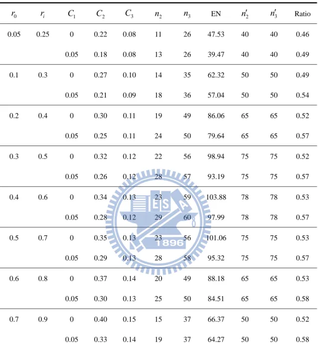
Table 1. Designs for ri r0 0.20, K 1,
K,
0.05,0.2
0 r ri C1 C2 C3 n2 n3 EN n2 n3 Ratio 0.05 0.25 0 0.22 0.08 11 26 47.53 40 40 0.46 0.05 0.18 0.08 13 26 39.47 40 40 0.49 0.1 0.3 0 0.27 0.10 14 35 62.32 50 50 0.49 0.05 0.21 0.09 18 36 57.04 50 50 0.54 0.2 0.4 0 0.30 0.11 19 49 86.06 65 65 0.52 0.05 0.25 0.11 24 50 79.64 65 65 0.57 0.3 0.5 0 0.32 0.12 22 56 98.94 75 75 0.52 0.05 0.26 0.12 28 57 93.19 75 75 0.57 0.4 0.6 0 0.34 0.13 23 59 103.88 78 78 0.53 0.05 0.28 0.12 29 60 97.99 78 78 0.57 0.5 0.7 0 0.35 0.13 23 56 101.06 75 75 0.53 0.05 0.29 0.13 28 58 95.32 75 75 0.57 0.6 0.8 0 0.37 0.14 20 49 88.18 65 65 0.53 0.05 0.30 0.13 25 50 84.51 65 65 0.58 0.7 0.9 0 0.40 0.15 15 37 66.37 50 50 0.52 0.05 0.33 0.14 19 37 64.27 50 50 0.58 2
n ans n3 is the sample size per group of our proposed design at the phase II and III stage correspondingly.
2
n
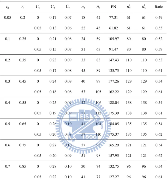
Table 2. Designs for ri r0 0.15, K 1,
K,
0.05,0.2
0 r ri C1 C2 C3 n2 n3 EN n2 n3 Ratio 0.05 0.2 0 0.17 0.07 18 42 77.31 61 61 0.49 0.05 0.13 0.06 22 45 61.82 61 61 0.55 0.1 0.25 0 0.21 0.08 24 59 105.97 80 80 0.52 0.05 0.15 0.07 31 63 91.47 80 80 0.59 0.2 0.35 0 0.23 0.09 33 83 147.43 110 110 0.53 0.05 0.17 0.08 45 89 135.75 110 110 0.61 0.3 0.45 0 0.24 0.09 40 99 177.26 129 129 0.54 0.05 0.18 0.08 53 105 162.22 129 129 0.61 0.4 0.55 0 0.25 0.09 42 106 188.04 138 138 0.54 0.05 0.19 0.09 57 112 175.39 138 138 0.61 0.5 0.65 0 0.26 0.10 41 104 184.05 135 135 0.54 0.05 0.20 0.09 57 110 175.37 135 135 0.62 0.6 0.75 0 0.27 0.10 37 93 165.29 121 121 0.54 0.05 0.20 0.09 51 98 157.95 121 121 0.62 0.7 0.85 0 0.28 0.10 30 74 132.75 96 96 0.54 0.05 0.22 0.10 41 77 127.27 96 96 0.61 2n ans n3 is the sample size per group of our proposed design at the phase II and III stage correspondingly. n2 ans n3 is the sample size per group of a traditional one-stage design at the phase II and III stage respectively.
Table 3. Designs for ri r0 0.20, K 2,
K,
0.05,0.2
0 r ri C1 C2 C3 n2 n3 EN n2 n3 Ratio 0.05 0.25 0 0.23 0.09 13 33 93.41 51 51 0.45 0.05 0.19 0.09 15 33 74.22 51 51 0.47 0.1 0.3 0 0.28 0.11 17 45 125.25 63 63 0.49 0.05 0.23 0.10 20 45 105.11 63 63 0.52 0.2 0.4 0 0.33 0.12 22 62 168.13 83 83 0.51 0.05 0.27 0.12 28 61 149.63 83 83 0.54 0.3 0.5 0 0.35 0.13 26 71 195.08 95 95 0.51 0.05 0.29 0.13 32 71 174.93 95 95 0.54 0.4 0.6 0 0.36 0.14 27 74 203.00 99 99 0.51 0.05 0.30 0.13 34 74 185.77 99 99 0.55 0.5 0.7 0 0.38 0.14 26 71 195.07 95 95 0.51 0.05 0.32 0.14 33 71 180.69 95 95 0.55 0.6 0.8 0 0.40 0.15 22 62 168.10 83 83 0.51 0.05 0.33 0.14 29 61 158.52 83 83 0.54 0.7 0.9 0 0.43 0.16 17 47 128.50 63 63 0.51 0.05 0.36 0.15 22 46 121.45 63 63 0.54 2n ans n3 is the sample size per group of our proposed design at the phase II and III stage correspondingly. n2 ans n3 is the sample size per group of a traditional one-stage design at the phase II and III stage respectively.
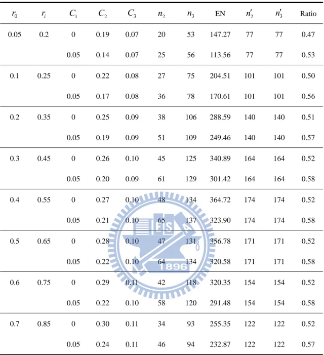
Table 4. Designs for ri r0 0.15, K 2,
K,
0.05,0.2
0 r ri C1 C2 C3 n2 n3 EN n2 n3 Ratio 0.05 0.2 0 0.19 0.07 20 53 147.27 77 77 0.47 0.05 0.14 0.07 25 56 113.56 77 77 0.53 0.1 0.25 0 0.22 0.08 27 75 204.51 101 101 0.50 0.05 0.17 0.08 36 78 170.61 101 101 0.56 0.2 0.35 0 0.25 0.09 38 106 288.59 140 140 0.51 0.05 0.19 0.09 51 109 249.46 140 140 0.57 0.3 0.45 0 0.26 0.10 45 125 340.89 164 164 0.52 0.05 0.20 0.09 61 129 301.42 164 164 0.58 0.4 0.55 0 0.27 0.10 48 134 364.72 174 174 0.52 0.05 0.21 0.10 65 137 323.90 174 174 0.58 0.5 0.65 0 0.28 0.10 47 131 356.78 171 171 0.52 0.05 0.22 0.10 64 134 320.58 171 171 0.58 0.6 0.75 0 0.29 0.11 42 118 320.35 154 154 0.52 0.05 0.22 0.10 58 120 291.48 154 154 0.58 0.7 0.85 0 0.30 0.11 34 93 255.35 122 122 0.52 0.05 0.24 0.11 46 94 232.87 122 122 0.57 2n ans n3 is the sample size per group of our proposed design at the phase II and III stage correspondingly. n2 ans n3 is the sample size per group of a traditional one-stage design at the phase II and III stage respectively.
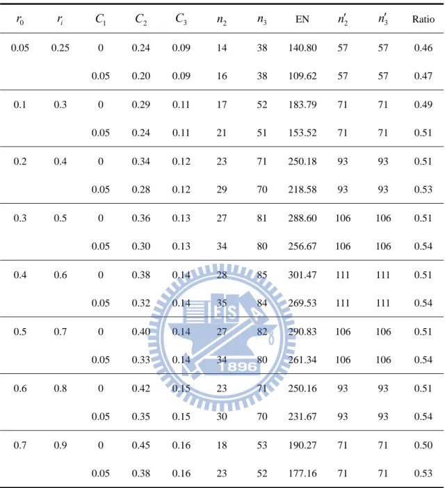
Table 5. Designs for ri r0 0.20, K 3,
K,
0.05,0.2
0 r ri C1 C2 C3 n2 n3 EN n2 n3 Ratio 0.05 0.25 0 0.24 0.09 14 38 140.80 57 57 0.46 0.05 0.20 0.09 16 38 109.62 57 57 0.47 0.1 0.3 0 0.29 0.11 17 52 183.79 71 71 0.49 0.05 0.24 0.11 21 51 153.52 71 71 0.51 0.2 0.4 0 0.34 0.12 23 71 250.18 93 93 0.51 0.05 0.28 0.12 29 70 218.58 93 93 0.53 0.3 0.5 0 0.36 0.13 27 81 288.60 106 106 0.51 0.05 0.30 0.13 34 80 256.67 106 106 0.54 0.4 0.6 0 0.38 0.14 28 85 301.47 111 111 0.51 0.05 0.32 0.14 35 84 269.53 111 111 0.54 0.5 0.7 0 0.40 0.14 27 82 290.83 106 106 0.51 0.05 0.33 0.14 34 80 261.34 106 106 0.54 0.6 0.8 0 0.42 0.15 23 71 250.16 93 93 0.51 0.05 0.35 0.15 30 70 231.67 93 93 0.54 0.7 0.9 0 0.45 0.16 18 53 190.27 71 71 0.50 0.05 0.38 0.16 23 52 177.16 71 71 0.53 2n ans n3 is the sample size per group of our proposed design at the phase II and III stage correspondingly. n2 ans n3 is the sample size per group of a traditional one-stage design at the phase II and III stage respectively.
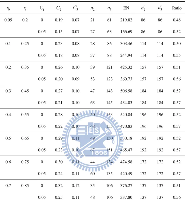
Table 6. Designs for ri r0 0.15, K 3,
K,
0.05,0.2
0 r ri C1 C2 C3 n2 n3 EN n2 n3 Ratio 0.05 0.2 0 0.19 0.07 21 61 219.82 86 86 0.48 0.05 0.15 0.07 27 63 166.69 86 86 0.52 0.1 0.25 0 0.23 0.08 28 86 303.46 114 114 0.50 0.05 0.18 0.08 37 88 244.94 114 114 0.55 0.2 0.35 0 0.26 0.10 39 121 425.32 157 157 0.51 0.05 0.20 0.09 53 123 360.73 157 157 0.56 0.3 0.45 0 0.27 0.10 47 143 506.58 184 184 0.52 0.05 0.21 0.10 63 145 434.03 184 184 0.57 0.4 0.55 0 0.28 0.10 50 153 540.84 196 196 0.52 0.05 0.22 0.10 68 155 470.83 196 196 0.57 0.5 0.65 0 0.29 0.11 49 150 530.18 192 192 0.52 0.05 0.23 0.10 67 151 465.47 192 192 0.57 0.6 0.75 0 0.30 0.11 44 134 474.58 172 172 0.52 0.05 0.24 0.11 60 135 420.49 172 172 0.57 0.7 0.85 0 0.32 0.12 35 106 376.27 137 137 0.51 0.05 0.25 0.11 48 106 337.80 137 137 0.56 2n ans n3 is the sample size per group of our proposed design at the phase II and III stage correspondingly. n2 ans n3 is the sample size per group of a traditional one-stage design at the phase II and III stage respectively.
Table 7. The result of simulation for the case of ri r0 0.20 , K 1 ,
K,
0.05,0.2
, C100
r ri Program_alpha Program_power Simulation_alpha Simulation_power
0.05 0.25 0.0505 0.7977 0.0827 0.9292 0.1 0.3 0.0507 0.7932 0.0646 0.8899 0.2 0.4 0.0505 0.7975 0.0557 0.8507 0.3 0.5 0.0505 0.7952 0.0512 0.8122 0.4 0.6 0.0505 0.7961 0.0489 0.7984 0.5 0.7 0.0499 0.7996 0.0492 0.7940 0.6 0.8 0.0499 0.8000 0.0496 0.7808 0.7 0.9 0.0500 0.8004 0.0511 0.7582
Table 8. The result of simulation for the case of ri r0 0.20 , 1K ,
K,
0.05,0.2
, C1 0.05, C2:two-sided0
r ri Program_alpha Program_power Simulation_alpha Simulation_power
0.05 0.25 0.0507 0.7966 0.0889 0.9287 0.1 0.3 0.0494 0.8020 0.0713 0.8824 0.2 0.4 0.0502 0.7995 0.0551 0.7966 0.3 0.5 0.0501 0.7980 0.0439 0.7924 0.4 0.6 0.0505 0.7964 0.0507 0.7991 0.5 0.7 0.0505 0.7975 0.0417 0.7610 0.6 0.8 0.0500 0.7995 0.0475 0.7825 0.7 0.9 0.0500 0.7987 0.0595 0.7856
Table 9. The result of simulation for the case of ri r0 0.15 , K 1 ,
K,
0.05,0.2
, C100
r ri Program_alpha Program_power Simulation_alpha Simulation_power
0.05 0.2 0.0505 0.7977 0.0305 0.8786 0.1 0.25 0.0507 0.7932 0.0480 0.8641 0.2 0.35 0.0505 0.7975 0.0474 0.8203 0.3 0.45 0.0505 0.7952 0.0482 0.8255 0.4 0.55 0.0505 0.7961 0.0532 0.8095 0.5 0.65 0.0499 0.7996 0.0503 0.7823 0.6 0.75 0.0499 0.8000 0.0497 0.7744 0.7 0.85 0.0500 0.8004 0.0553 0.7889
Table 10. The result of simulation for the case of ri r0 0.15 , 1K ,
K,
0.05,0.2
, C1 0.050
r ri Program_alpha Program_power Simulation_alpha Simulation_power
0.05 0.2 0.0508 0.7974 0.0485 0.7910 0.1 0.25 0.0505 0.7975 0.0581 0.8382 0.2 0.35 0.0501 0.7983 0.0550 0.8054 0.3 0.45 0.0506 0.7958 0.0616 0.8209 0.4 0.55 0.0505 0.7960 0.0480 0.7996 0.5 0.65 0.0500 0.7986 0.0462 0.7916 0.6 0.75 0.0503 0.7971 0.0523 0.7974
Figures
Figure 1. Simulated success rates for the case of ri r0 0.20 , K 1 ,
K,
0.05,0.2
, C10Figure 2. Simulated success rates for the case of ri r0 0.20 , K 1 ,
K,
0.05,0.2
, C1 0.05Figure 3. Simulated success rates for the case of ri r0 0.15 , K 1 ,
K,
0.05,0.2
, C10Figure 4. Simulated success rates for the case of ri r0 0.15 , K 1 ,
K,
0.05,0.2
, C1 0.05Appendix
According to the assumption that the estimates of response rates at the phase II stage of the dose groups and the control group are mutually independent and the result of Central Limit Theorem, (rˆ0II,rˆ1II,...,rˆKII)T follows a multivariate normal distribution,
2 2 1 1 2 0 0 1 1 1 0 1 1 1 1 0 1 0 1 0 1 , ~ ˆ ˆ ˆ 0 n r r n r r n r r r r r N r r r K K K K K K K H II K II II .Since (X1,X2,...,XK)T can be expressed as A(rˆ0II,rˆ1II,...,rˆKII)T where
0 2
1 2 0 2 2 0 1 1 1 0 0 1 0 1 0 1 0 0 1 1 , , 1 0 , , 1 0 , , 1 A K K K K K K K n r r n r r n r r ,we can conclude that
, ~ ) ,..., , (X1 X2 XK T NK because of the property of the multivariate normal distribution, where
2 0 0 2 0 2 0 2 2 0 1 0 1 , , , , , , A n r r r r n r r r r n r r r r K K and
2 0 2 2 2 0 0 2 0 2 0 2 2 0 0 2 0 2 0 1 2 0 0 2 0 2 0 2 2 0 0 2 0 2 2 2 2 2 2 0 0 2 0 2 2 0 1 2 0 0 2 0 2 0 1 2 0 0 2 0 2 2 0 1 2 0 0 2 0 1 2 2 1 1 2 0 0 , , 1 1 , , , , 1 , , , , 1 , , , , 1 , , 1 1 , , , , 1 , , , , 1 , , , , 1 , , 1 1 A A n r r n r r n r r n r r n r r n r r n r r n r r n r r n r r n r r n r r n r r n r r n r r n r r n r r n r r n r r n r r n r r n r r n r r n r r n r r n r r n r r K K K K K K K T .Therefore, under the null hypothesis that ri r0 0, we can get that
1 2 1 2 1 2 1 1 2 1 2 1 2 1 1 , 0 0 0 ~ ) ,..., , ( 0 2 1 K H T K N X X X .
References
1. Maca, J. Bhattacharya, S. Dragalin, V. Gallo, P. Krams, M. (2006). Adaptive seamless phase II/III designs : Background, operational aspects, and examples.
Drug Information Journal, 40, 463-473.
2. Simon, R. (1989). Optimal two-stage designs for phase II clinical trials,
Controlled Clinical Trials, 10, 1-10.
3. Tsou, H. H., Hsiao, C. F., Chow, S. C., and Liu, J. P. (2008). A two-stage design for drug screening trials based on continuous endpoints, Drug Information
Journal, 42, 253-262.
4. Schaid, D. J. Wieand, S. and Therneau, T. M. (1990). Optimal two-stage screening designs for survival comparisons, Biometrika, 77, 507-13
5. Scher, H. I. and Heller, G. (2002) Picking the winners in a sea of plenty, Clinical
Cancer Research, 8,400-404
6. Liu Q, Pledger GW. Phase II and III combination designs to accelerate drug development. J Am Stat Assoc. 2005;100:493-502.
7. Kelly PJ, Stallard N, Todd S. An adaptive group sequential design for phase II/III clinical trials that select a single treatment from several. J Biopharm Stat. 2005;15:641-658.
8. Gupta, S. S.(1963). Probability integrals of multivariate normal and multivariate t.
Ann. Math. Statist. 34, 792-828.
9. Shein-Chung Chow, Mark Chang (2006). Adaptive design methods in clinical trials.