降低網路控制系統資料傳輸率之研究

(1)

國立交通大學

電機與控制工程學系

碩士論文

降低網路控制系統資料傳輸率之研究

Study on Data Transmission Rate Reducing of Networked

Control Systems

研究生 : 黃逸幗

指導教授 : 李祖添博士

(2)

降低網路控制系統資料傳輸率之研究

研究生:黃逸幗指導教授:李祖添博士

國立交通大學電機與控制工程系碩士班

摘要

論文內容將探討網路控制系統伴隨傳送延遲的問題。網路產生的傳輸延遲往往會對網路控制閉迴路造成負面的影響,例如:降低系統的穩定度和造成控制效能變差。論文中將會先引入未考慮網路狀況的單一直流馬達系統，然後針對此一單一系統用極點位移的方式設計控制器。最後再將設計出來的控制器加上網路系統完成整個系統的架構。網路造成的延遲可大致分為兩種:一種是固定的延遲, 另一種是隨機的延遲，本論文將探討前者對網路控制系統的影響。我們為了降低網路的使用率，使網路發揮更大的功能並且維持整個控制系統的穩定性，我們將訂出一個傳輸誤差的範圍，控制行為將依據此一標準來決定控制行為。系統中央控制器會根據最新的系統狀態來決定是否更新控制命令，傳輸誤差的範圍也是跟系統最新狀態有關。根據此控制法則，可以降低耗用之網路資源並且保證系統的穩定度。系統傳輸誤差是網路實際應用上的一種無法避免的現象且將會於文中定義。模擬將會以兩個不同直流馬達和線性不穩定系統來作驗證。文中也將討論網路產生延遲的影響。

(3)

Study on Data Transmission Rate

Reducing of Networked Control

Systems

Student: Yi-Kuo Huang Advisor: Tsu-Tian Lee

Department of Electrical and Control Engineering

National Chiao Tung University

ABSTRACT

A network system considering network-induced delay is presented in this thesis. Network-induced delay may have advert influences on networked closed-loop control system such as performance degradation and system destabilization. We will first introduce single DC motor plant without considering networked control systems, and design individual controller for DC motor using pole placement method. Then, the overall networked control systems will be introduced. There are two types of network-induced delay: one is fixed delay; the other is random delay. The former is adopted in the thesis. In order to reduce network usage and maintain system stability, control input signals are sent under certain boundary conditions. Central controller sends control signals according to present states or former control states of the plants. The network usage can be reduced and overall system stability can be guaranteed, too. Transmission error is a practical phenomenon in NCS and will be defined in the thesis. Examples of controlling two DC servo-motors or two linear unstable systems through network will be demonstrated, and the effects caused by network-induced delay will also be shown in simulations and discussed in the thesis.

(4)

誌謝

首先很感謝指導教授李祖添校長還有吳政郎教授的耐心指導，讓我能順利完成這本論文。也謝謝口試委員謝哲光教授和張隆國教授的斧正。交大的六年生活，充滿了喜怒哀樂的回憶，很慶幸身邊一直有好朋友陪伴跟幫助。在碩士生活的這兩年，更是讓我學習成長不少，實驗室學長同學的關心跟體貼讓我永記心中，誰說唸理工的人都很冷冰冰呢! 最後感謝家人跟男友一路的支持跟鼓勵，她們給了我精神上最大的幫助。本文謹獻給 805 實驗室: 欣翰學長、炳榮學長、冠銘學長、保村學長、文真、雅齡、詠建、東璋，謝謝你們。

(5)

CONTENTS 摘要 i ABSTRACT ii 誌謝 iii CONTENTS iv LIST OF FIGURES v

LIST OF TABLES viii

CHAPTER 1 INTRODUCTION 1

1.1 Motivation 1

1.2 Survey of DC Motor Systems and Unstable Systems 1 1.3 Survey of Pole Placement and Lyapunov Stability 2 1.4 Survey of Network Control Systems 3 1.5 Thesis Organization and Contributions 4

CHAPTER 2 SYSTEM MODEL 5

2.1 System Model 5

2.1.1 DC Motor Systems and Unstable Systems 5 2.1.2 Network System Model 7

CHAPTER 3 POLE PLACEMENT DESIGN METHODOLOGY 10

3.1 Pole Placement Theory 10

3.2 Design Algorithm 10

3.3 Simulations of DC Motor Systems and Unstable Systems 14

CHAPTER 4 NETWORK STABILITY ANALYSIS 22

4.1 Lyapunov Stability Theory 22

4.2 Modified Lyapunov Stability with Network Conditions 23 4.3 Simulations

4.3.1 Network Control System without Delay 34

4.3.2 Network Control System with Delay 37

CHAPTER 5 CONCLUSIONS 40

5.1 Remark Conclusions 40

5.2 Future Work 41

(6)

LIST OF FIGURES

Fig. 1.1 A typical NCS setup and information flow 3 Fig. 2.1 Equivalent circuit of the DC motor 5 Fig.. 2.2 Control network system structure with induced delay 8 Fig. 3.1 The relation between ωn and ξ when ts =0.1s, tr =0.07s, and

12

s td =0.06

Fig. 3.2 The relation of ω_n and ξ when three design condition are all satisfied. 12 Fig. 3.3(a) The relation between ωn and ξ when ts =0.059 , and

15 01 . 0 = d t 02 . 0 = r t

Fig. 3.3(b) The output angular speed of controlled (red line) and uncontrolled (blue line)

System 1 16

Fig. 3.3(c) The output angular speed of controlled (red line) and uncontrolled (blue line)

System 2 16

Fig. 3.4(a) The relation between ω_n and ξ when t_s =0.03, 008t_d =0. and t_r =0.01

17 Fig. 3.4(b) The output angular speed of controlled (red line) and uncontrolled (blue line)

System 1 17

System 2 17

Fig. 3.5(a) The relation between ω_n and ξ when t_s =0.02009, and 18 003 . 0 = d t 005 . 0 = r t

Fig. 3.5(b) The output angular speed of controlled (red line) and uncontrolled (blue line)

System 1 18

System 2 18

Fig. 3.6(a) The relation between ωn and ξ when ts =12, 2td = and tr =4 19

Fig. 3.6(b) The output of controlled and uncontrolled unstable System 1 19 Fig. 3.6(c) The relation between ωn and ξ when ts =7, 1td = and tr =2 20

(7)

Fig. 3.7(a) The relation between ωn and ξ when ts =10, 1td = and tr =3 21

Fig. 3.7(b) The output of controlled and uncontrolled unstable System 1 21 Fig. 3.7(b) The output of controlled and uncontrolled unstable System 2 21 Fig. 3.8(a) The relation between ω_n and ξ when t_s =2.5, 5t_d =0. and t_r =1 22 Fig. 3.8(b) The output of controlled and uncontrolled unstable System 1 where ωn =4

and ξ =0.98 22

Fig. 3.8(c) The output of controlled and uncontrolled unstable System 2 where ω_n =4

and 98ξ =0. 22

Fig. 4.1 Transmission error bound 24

Fig. 4.2 Transmission error bound and control states 26 Fig. 4.3 Transmission error bound and control states of NCS with delays 30 Fig. 4.4 The controlling block diagram of overall networked system 33 Fig. 4.5(a) The angular velocity of transition error controlled and uncontrolled system

of System1 34

Fig. 4.5(b) The angular velocity of transition error controlled and uncontrolled system

of System2 34

Fig. 4.5(c) The controlled frequencies of DC motor ststem1 and system2 35 Fig. 4.6(a) The output of transition error controlled and uncontrolled system of Unstable

system1 35

Fig. 4.6(b) The output of transition error controlled and uncontrolled system of Unstable system2 35 Fig. 4.6(c) The controlled frequencies of Unstable sytem1 and system2 36 Fig. 4.7(a) The angular velocity of transition error controlled with delays and

uncontrolled system of System1 36

Fig. 4.7(b) The angular velocity of transition error controlled with delays and

uncontrolled system of System2 37

Fig. 4.7(c) The controlled frequencies of DC motor ststem1 and system2 with delays. 37 Fig. 4.8(a) The output of transition error controlled with delays and uncontrolled system

(8)

Fig. 4.8(b) The output of transition error controlled with delays and uncontrolled system

of Unstable system2 38

Fig. 4.8(c) The controlled frequencies of Unstable sytem1 and system2 with delays. 38

(9)

LIST OF TABLES

Table 3.1 ITAE values according to different combinations of ξand ωn 13

Table 3.2 The parameters of DC motors systems 15 Table 3.3 ITAE of System 1 and System 2 according to possible ξ and ωn

combinations 15

Table 3.4 ITAE of System 1 and System 2 according to possible ξ and ω_n

combinations 16

Table 3.5 ITAE of unstable System 1 and System 2 according to possible ξand

n

ω combination 19

Table 3.6 ITAE of unstable System 1 and System 2 according to possible ξand

n

(10)

CHAPTER 1 INTRODUCTION

1.1 Motivation

The overwhelming stands of network system are obviously in recent decades. Because of the complexity and loads are rapidly increasing, the demands of NCS’s performance are ever increasing. A system without network system can only control one sub-plant, while a well-designed network control system can deal with ten times or more sub-plants with only one central controller. The efficiency is distinctly superior than the traditional control systems in many ways. Furthermore, the applications connected through a network can be remotely controlled from a long–distance source. Conventionally, the networks used in the aforementioned applications are specific industrial networks, such as CAN (Controller Area Networks), and PROFIBUS. However, general data networks such as Ethernet and Internet are quickly advancing to be the networks of choices for many applications due to their flexibility and lower costs. There are two general structures to design a control system through a network. The first structure is to have several sub-systems, in which each of them contains a set of sensors, actuators, and a controller by itself. These system components are attached to the same control plant. In this case, a sub-system controller receives a set point from the central controller. Another structure is to connect a set of sensors and actuators to a network directly. Sensors and actuators in this case are attached to a plant, while a controller is separated from the plant via a network connection to perform a closed-loop control over the network. In this thesis, the latter is adopted.

In order to extend the network efficiently, we try to provide a simple but useful methodology to reduce the usage of the network. The network induced time delays are also topic to be discussed. Therefore, under allowable physical condition, we can enlarge the control network as large as possible and display the influences brought by network delays [14].

1.2 Survey of DC Motor Systems and unstable Systems

Two kinds of sub-systems will be used in this thesis. One is DC motor servo systems, and the other is a random selected linear unstable system. Those two different sub-systems will demonstrate distinct results: as for the unstable system, we will focus more on system stability, and the DC motor servo systems, we will emphasize more on

(11)

the transient performances.

In recent years, the use of DC machines has become exclusively associated with applications where the unique characteristics of the DC motor (i.e., high starting torque for traction motor application) justify its cost, or where portable equipment must be run from a DC (or battery) power supply. The ease with which the DC motor lends itself to speed control has long been recognized. Compatibility with transistor amplifiers, plus better performance due to the availability of new improved materials in magnets, brushes and epoxies, has also revitalized interest in DC machines. The need for new high-performance motors with highly sophisticated capabilities has produced a superabundance of new shapes and sizes quite unlike DC machines years ago.

The DC motors are original convergent systems, and therefore we will put emphases on their transient performances than stability conditions. The related reference of DC motor control through network system is [15].

1.3 Survey of Pole Placement and Lyapunov Theory

Pole placement is a traditional control system design technique for linear time-invariant control systems. The technique is based on the fact that several performance specifications can be met using dynamic output feedback to adequately place closed-loop poles in the complex plane. An extension of the classical pole placement problem is the regional pole placement problem, in which the objective is to place closed-loop poles in a suitable region of the complex plane. The regional pole placement problem is usually treated in connection with the substantially more general problem of placing closed-loop poles in a specified region in the face of uncertainty with respect to the mathematical model of the plant. In many real-world situations, the model uncertainty reflects on the parameters of the plant, which has motivated extensive research efforts in parametric robust control theory [10]-[12].

Lyapunov stability theory is more often used in analyzing nonlinear systems than linear systems [13]. In this thesis, Lyapunov theory is adopted to solving the stability problem of system with network condition added. A transmission error bound is derived from Lyapunov stability conditions [21].

1.4 Survey of Network Control Systems

Feedback control systems wherein the control loops are closed through a real-time network are called networked control systems (NCSs) [1-4 and 18]. The defining

(12)

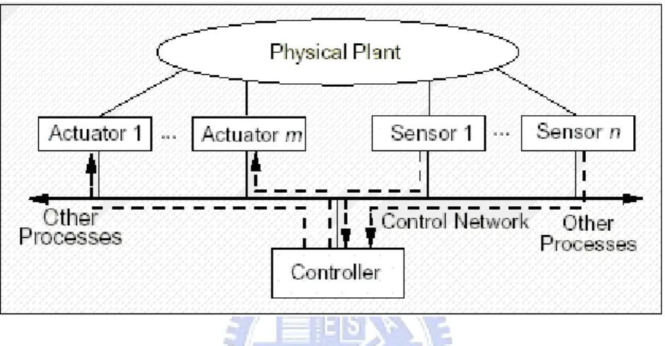
feature of an NCS is that information (reference input, plant output, control input, etc.) is exchanged using a network among control system components (sensors, controller, actuators, etc.). Fig.. 1.1 illustrates a typical setup and the information flows of an NCS. The primary advantages of an NCS are reduced system wiring, ease of system diagnosis and maintenance, and increased system agility. The insertion of the communication network in the feedback control loop makes the analysis and design of an NCS complex. Conventional control theories with many ideal assumptions, such as synchronized control and non-delayed sensing and actuation, must be reevaluated before they can be applied to NCSs.

Fig. 1.1 A typical NCS setup and information flows

Specifically, the following issues need to be addressed. The first issue is the network-induced delay (sensor-to-controller delay and controller-to-actuator delay) that occurs while exchanging data among devices connected to the shared medium. This delay, either constant or time varying, can degrade the performance of control systems designed without considering the delay and can even destabilize the system[16][19][20].

The network can be viewed as a web of unreliable transmission paths. Some packets not only suffer transmission delay but, even worse, can be lost during transmission. Thus, how such packet dropouts affect the performance of an NCS is an issue that must be considered.

Another issue is that plant outputs may be transmitted using multiple network packets (so-called multiple-packet transmission), due to the bandwidth and packet size constraints of the network. Because of the arbitration of the network medium with other nodes on the network, chances are that all/part/none of the packets could arrive by the time of control calculation.

(13)

network-induced delays in the direction from controller to actuators. Many researches have been done when it comes to discuss about the problems of network-induced delays. Some of them focus on finding the transmission deadlines for which the stability of the NCS is guaranteed [3,4,7, and 14].

1.5 Thesis Organization and Contributions

This thesis has been organized as follows. Chapter 2 introduces the system model including sub-systems and overall models. Chapter 3 presents the pole placement controller design procedures and results. Chapter 4 briefs Lyapunov stability and the main proof of error bound results. Chapter 5 gives the simulation results of Chapter 4. Chapter 6 concludes the thesis also highlighting future studies of NCS.

The stability of error bound promising system is derived in this thesis. The central controller can spare more time dealing with other sub-plants. In this way, the central controller only needs to send control signals less than 250 times during 5000 times accessing to the network of the least control times. In other words, ten times the sub-plants can be inserted as long as the physical layer of NCS could afford.

(14)

CHAPTER 2 SYSTEM MODEL

2.1 System Model

The whole system is composed of two different sub-systems: DC motors and network part. We will first present DC motor models in mathematical form in section 2.1.1 and then the overall system in section 2.1.2 with the network system plugged in.

2.1.1 DC motor systemand Unstable Systems

In this chapter, two DC motor systems are chosen as control plants. For a long time, motor system is always a very fundamental but crucial system. No matter in theoretically proving or practical implementation, because of their simplicity in structure and malleability in function, they are widely used in system analysis, design and application. We will introduce the mathematical model of a single motor, and then the whole motor system.

The motor is a machine devises electrical power into mechanical power; more specifically it transfers electrical power into mechanical power with the help of magnetic field. Since the magnetic field is always constant, it is not our subject to discuss the relating problem in this field. We will focus on the relation between electrical power and mechanical power. Moreover, many useful mathematical models would be constructed as follows.

Equation of electrical model of the motor is given by:

g a a a R I E dt dI L V = ⋅ + ⋅ + (2-1) R La M Motor + -Tg,w V Ia Eg

Fig. 2.1 Equivalent circuit of the DC motor

where and are the motor voltage and current respectively. The motor impedance at stall is equal to a combination circuit of resistance,

V I_a

(15)

g

E is the internally generated voltage which is proportional to the motor velocity, ω .

ω ⋅ = _E

g K

E (2-2)

Combining (2-1) and (2-2), we have the electrical equation ω ⋅ + ⋅ + ⋅ = a E a a R I K dt dI L V (2-3) Second, we will introduce motor dynamic equation. The relation between torques and velocity is given by

L m g T T dt d J T = ⋅ ω + + (2-4)

where is the total moment of inertia, is the internally generated torque, and is the load opposing torque. The opposing torque in the motor is given by

J Tg L T f m D T T = ⋅ω + (2-5)

where is the viscous damping factor, and is the internal friction torque. Because of the constant magnetic field, the current produces a proportional torque

D T_f

a T

g K I

T = ⋅ (2-6) where is the torque constant. Therefore, the total dynamic function from (2-4), (2-5) and (2-6) are T K L f a T D T T dt d J I K ⋅ = ⋅ ω + ⋅ω+ + (2-7) For simplicity, we will assume that motor velocity is the same as that of the load. The following results are based on the equal velocity definition. Finally, linking up motor electric equation (2-3), (2-4) and motor dynamic equation (2-7), we have a motor mathematical model with its variables. However, a transfer function is needed when we want to design a control system. The relations between input signals and output signals are easier to understand in this way. We assume T_f =0 and TL =0

(16)

for further discussion since neither of them affect the transfer function. The Laplace transforms of the motor equations are

) ( ) ( ) ( ) (s s L R I s K s V = ⋅ _a + ⋅ _a + _E ⋅ω (2-8) ) ( ) (s D s s J I KT ⋅ a⋅= ⋅ ⋅ω + ⋅ω (2-9)

We can obtain an expression for the current:

) ( ) ( 1 ) ( s J D s K s I T a = ⋅ + ⋅ω (2-10)

If we combine (2-8) and (2-10), we have

) ( ) ( ) )( ( 1 ) ( s L R s J D s K s K s V a E T ω ω + ⋅ ⋅ + ⋅ + ⋅ = (2-11)

For simplicity, we let damping factor negligible, and the corresponding transfer function becomes

D T E a T m K K J R s J L s K s V s s G ⋅ + ⋅ ⋅ + ⋅ ⋅ = = ₂ ) ( ) ( ) ( ω (2-12)

As mention to unstable systems, virtual linear unstable systems are adopted in this thesis. Purposely, we build up a linear system with locating its poles on the right hand side of complex plant. Because of the innate physical characteristics, DC motors are always convergent. Therefore, the linear unstable systems are used for comparison with DC motor systems.

2.1.2 Network system model

Traditionally, point-to-point communication architecture for control system has

been used for decades in industry. However, enormously growing physical setups and functionality both test the limits of point-to-point communication architecture. Network systems with common bus architectures, called networked control systems (NCSs), have many advantages such as small volume of wiring and distributing processing. Those merits make it possible to implement larger communication architecture ever.

There are three typical network architectures using control communication- Ethernet, Control net, and Device net. In this paper, we choose Device net (CAN bus) as our NCS architecture. CAN bus is a deterministic protocol optimized for short messages, and the message priority is specified in the arbitration field, which means the network-induced delay is predictable and probably is some fixed constant. The

(17)

disadvantages of CAN are limited data rate (maximum of 500 Kb/s) and limited size of transferring data. However, these demerits do not cause any problem to the following discussion.

Several network-based controlled DC motors are used as an example to demonstrate the effectiveness of the proposed scheme. The whole system is composed of three different units: plant (DC motors), central controller, and communication network (CAN bus). The structure is shown in Fig.. 2.1. We concern the CAN as the only time delay part, and the control input signal delay is introduced between central controller and motor controller through CAN bus.

Central PC Control

motor

Actuator & Sensor

motor delay

delay

. . . .

Fig.. 2.2 Control network system structure with induced delay

Now, we want to know some performance and characteristics of the plant. It is very intuitive to find a state space representation of the target system. A common form of state space of a motor is given by

) ( ) ( ) (t A x t B u t x& = ⋅ + ⋅ (2-13) where x=

[

x1 x2

]

T is the state, and y is the output. We take x1 =ω (rpm), ,

(volt) into (2-12). We also choose motor speed as the single output, where

1 2 x x = & V u= ⎥ ⎥ ⎦ ⎤ ⎢ ⎢ ⎣ ⎡ − ⋅ ⋅ − = a a T E L R J L K K A 1 0 , ⎥ ⎥ ⎦ ⎤ ⎢ ⎢ ⎣ ⎡ = a T L K B 0 (2-14)

Next, we will consider some realistic situations of the network systems. For instance, the feedback states are not always available, and therefore the control input may be not compatible to the present condition. To illustrate the situation, rewrite the

(18)

input part in the state space of (2-13) as ) ( ) ( ) (t A x t B u t_k x& = ⋅ + ⋅ , where t₀ <t_k ≤t (2-15) The symbol represents some time point that before the present time, and is the initial time. Another Delay time will also be put into mathematical expression. We assume that delay time is a fixed constant, say

k t t0 τ , and (2-15) becomes ) ( ) ( ) (t = A⋅x t +B⋅u t_k −τ x& (2-16) We are going to discuss how those situations influence the stability of the controlled plant in Chapter 4. In order to maintain stability, some bounds are required.

(19)

CHAPTER 3

POLE PLACEMENT DESIGN METHODOLOGY

3.1 Pole Placement Theory

There are many solutions to design a linear controller. One of the very direct controller design solution is pole placement that deals with the closed-loop poles and the system performance. In linear controller system design, the characteristics of a system can be easily shown by the location of closed-loop poles. Therefore, it is very intuitively to design a controller according to this strategy. We can effectively carry out the design by specifying the location of these poles. Firstly, the controller is designed without considering the presence of network. Besides, the controller dynamics is considered continuous because the access interval of the NCS to the network is much larger than the processing period of the controller and smart sensors.

To investigate the condition required for arbitrary pole placement in an n-th order system, we first consider that the process is described by (2-13), where is a state vector, and is the scalar control. The state feedback control is

) (t x n×1 ) (t u ) ( ) (t F x t u =− ⋅ (3-1) The pole placement method sustains under some conditions are also satisfied. The sufficient condition of pole placement is that the system must be controllable, which means (3-2) must have full rank.

[

B AB A2B .... An−1B

]

(3-2) A matrix exists that can give an arbitrary set of closed-loop poles of

. That is, the n roots of the characteristic equation

F ) (A−B⋅K 0 ) ( − ⋅ = − ⋅I A B F s (3-3) can be arbitrary placed. In order to discuss the connection between system characteristics and the pole placement method, we need to connect them with pole locations. From [6], we know that

n X ω θ ζ = cos = (3-4) 2 2 Y X n = + ω (3-5)

(20)

where X , Y are real part and imaginary part of the dedicated poles. θ is an angle

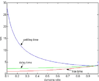
spanning from negative real axis to positive imaginary axis, and ξ is the damping ratio. Many system performances are closely related to these two factors such as rise time, delay time, settling time and overshoot. Their equations are already derived in [6] as follows: ) 1 10 ln( 1 ζ2 ζ ω ⋅ − − = −m n ts (3-6) n tr ω ζ ζ 2 917 . 2 4167 . 0 1− + = (3-7) n td ω ζ ζ 2 469 . 0 125 . 0 1 . 1 + + = (3-8) 2 1 ) ( _ ζ πζ − − ⋅ = finalspeed e shoot over (3-9)

Settling time means that the time when the output value first stayed within of the final value and always stayed in the range from the time on; rise time refers to the time period counts from the output value reaches 10% to 90% of the final value; delay time mentions the time when the output value reaches 50% of the final value. We will always keep damping ratio approach ‘1’ to avoid damping.

m

−

10

It is very clearly that as long as the system performances are constrained the locations of poles are also decided. We can choose the locations of desired system poles according to pre-limited conditions. In this thesis, we choose settling time, delay time and rise time as the design objective. But more conditions are needed in finding more specific pole location. We will discuss more in the next section.

3.2 Design Algorithm

There are several ways of pole placement such as identical radius, identical real, identical damping ratio. In this thesis, poles are assigned to have identical radius and damping ratio. In other words, poles are placed in the form of complex conjugate pairs. To arrange the locations of poles, in traditional pole placement design, most results came from thousands of trial and error tests. To have a more efficient design algorithm, first of all, it is necessary to make sure of system characteristics, settling time, delay time, rise time and overshoot, according to designer’s demands. For example, choose

0.1(sec.), (sec.), and =

s

(21)

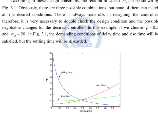
Fig. 3.1 The relation between ω_n and ξ when t_s =0.1s, t_r =0.07s, and t_d =0.06s

According to these design constrains, the relation of ξand ω_ncan be shown by Fig. 3.1. Obviously, there are three possible combinations, but none of them can match all the desired conditions. There is always trade-offs in designing the controller, therefore, it is very necessary to double check the design condition and the possible negotiable changes for the desired controller. In this example, if we choose ξ =0.5 and 20ω_n = in Fig. 3.1, the demanding conditions of delay time and rise time will be satisfied, but the settling time will be discarded.

Fig. 3.2 The relation of ω_n and ξ when three design condition are all satisfied

It is also possible that the three lines are intersected on one point, therefore, the design will have a perfect match of the design demands. In Fig. 3.2, three demands of the design are satisfied because the three lines have only one solution. In this case, we don’t need any further selection for the suitable pair of ξand ω . However, the case in

(22)

Fig. 3.1 is more common than the case in Fig. 3.2. This is why we need further examination of the selection of ξand ωn pair.

We will introduce another widely used error estimation standard called ITAE (Integral of Time multiplied by the Absolute Error) to do further selection of ξand

n

ω combinations for our design, and the equation of ITAE is given by

∫

⋅ ⋅

= t e t dt

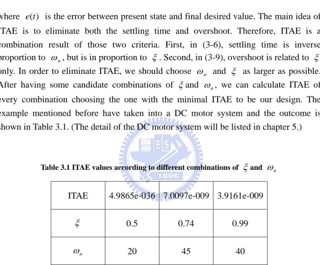
ITAE ( ) (3-10) where is the error between present state and final desired value. The main idea of ITAE is to eliminate both the settling time and overshoot. Therefore, ITAE is a combination result of those two criteria. First, in (3-6), settling time is inverse proportion to

) (t

e

n

ω , but is in proportion to ξ. Second, in (3-9), overshoot is related to ξ only. In order to eliminate ITAE, we should choose ω_n and ξ as larger as possible. After having some candidate combinations of ξand ω_n, we can calculate ITAE of every combination choosing the one with the minimal ITAE to be our design. The example mentioned before have taken into a DC motor system and the outcome is shown in Table 3.1. (The detail of the DC motor system will be listed in chapter 5.)

Table 3.1 ITAE values according to different combinations of ξand ω_n

ITAE 4.9865e-036 7.0097e-009 3.9161e-009

ξ 0.5 0.74 0.99

n

ω 20 45 40

Because of different system demands, the selection of poles is certainly very different. ITAE is just a kind of the selection standard, and one also can use minimal input or no damping standard as the design conditions. In this thesis, the settling time, rise time, delay time and ITAE standards are adopted in design controllers. Unlike the other pole placement methods proposed, we use a more specific way to eliminate the possible combinations of desired poles in the pole placement design algorithm. We combine conventional pole placement and ITAE to select desired locations of poles. The design algorithm not only can reduce the time wasted in finding suitable poles but can also meet design standard.

(23)

3.3 Simulations of DC Motor Systems and Unstable Systems

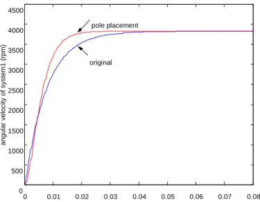
Two different DC (SYSTEM 1 and SYSTEM 2) motors are used as model systems. The state space of the DC motor system is shown in (1-13) and (1-14), where the parameters are listed in Table 3.2. We will demonstrate different design conditions and also show DC motor output results. The purpose of DC motor controller is speed control. System 1 and System 2 are two different DC motors. The latter is a high speed DC motor. The final speed of System 1 is set to fix at 3819.7 rpm (400 rad/s) and of System 2 is 6684.5 rpm (700 rad/s).

There are also two different unstable systems whose system models are given as follows according to (2-14). The poles are set to be s =-2.5,1.2 and , respectively. 10 0.6, = s

Linear unstable system 1:

) ( ) ( ) (t A x t B u t x& = ⋅ + ⋅ where _⎥ and . ⎦ ⎤ ⎢ ⎣ ⎡ − − − = 7 . 0 2 8 . 0 2 A _⎥ ⎦ ⎤ ⎢ ⎣ ⎡ = 1 1 B

) ( ) ( ) (t A x t B u t x& = ⋅ + ⋅ where _⎥ and . ⎦ ⎤ ⎢ ⎣ ⎡ = 10 3 1 1 A _⎥ ⎦ ⎤ ⎢ ⎣ ⎡ = 2 1 B

Examples of different intersecting points of settling time, rise time and delay time will be demonstrated. Fig. 3.3(a)~(c) and Table 3.3 show the design results of

, and . Fig. 3.4(a)~(c) and Table 3.4 show the results of , and . Fig. 3.5(a)~(c) and Table 3.5 show the results of

, and 059 . 0 = s t t_d =0.01 t_r =0.02 03 . 0 = s t t_d =0.01 t_r =0.008 02009 . 0 = s

t t_d =0.005 t_r =0.003. Fig. 3.6~Fig. 3.8 and Table 3.6~3.8 are design results of unstable systems, and are with corresponding design demands of Fig. 3.3~Fig. 3.5 and Table 3.3~3.5.

This algorithm could give the designer an approaching region of possible poles. Although the settling time, delay time, rise time and ITAE could guarantee some performances, it always needs some trial and error work to rectify the final locations of designed poles.

(24)

Table 3.2 The parameters of DC motors systems

SYSTEM 1 SYSTEM 2

Symbol Value Value

R (Ω ) 19.16 1.3 a L (m) 3 10 88 . 4 × − 3.4×10−4 m τ (sec.) 3 10 8× − 8×10−3 J(kgm2) 6 10 5 . 8 × − 8.5×10−6 T K (Nm /A) 0.145 2 10 82 . 3 × −

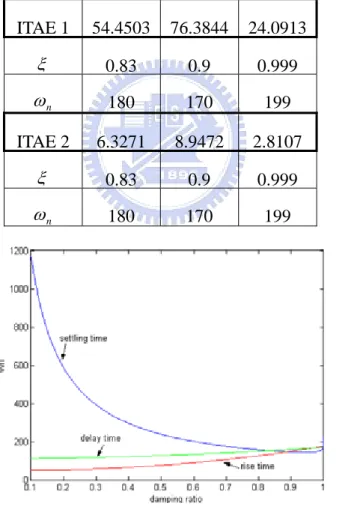
Table 3.3 ITAE of System 1 and System 2 according to possible ξand ω_n combinations

ITAE 1 54.4503 76.3844 24.0913 ξ 0.83 0.9 0.999 n ω 180 170 199 ITAE 2 6.3271 8.9472 2.8107 ξ 0.83 0.9 0.999 n ω 180 170 199

(25)

0 0.01 0.02 0.03 0.04 0.05 0.06 0.07 0.08 0 500 1000 1500 2000 2500 3000 3500 4000 4500 Ti a n g u lar v e locity of syst e m 1 ( rpm ) original pole placement

Fig. 3.3(b) The output angular speed of controlled (red line) and uncontrolled (blue line) System 1

0 0.01 0.02 0.03 0.04 0.05 0.06 0.07 0.08 0 1000 2000 3000 4000 5000 6000 7000 an g u la r v e lo city o f sy ste m 2 ( rpm ) original pole placement

Fig. 3.3(c) The output angular speed of controlled (red line) and uncontrolled (blue line) System 2

Table 3.4 ITAE of System 1 and System 2 according to possible ξand ωn combinations

ITAE 1 5.7533 177.2367 ξ 0.6 0.9 n ω 300 450 ITAE 2 0.5289 7.7748 ξ 0.6 0.9 n ω 300 450

(26)

Fig. 3.4(a) The relation between ω_n and ξ when t_s =0.03, t_d =0.008and t_r =0.01

(27)

Fig. 3.5(a) The relation between ω_n and ξ when t_s =0.02009, t_d =0.003and t_r =0.005

(28)

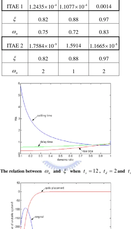
Table 3.5 ITAE of unstable System 1 and System 2 according to possible ξand ωncombination ITAE 1 -4 10 1.2435× 1.1077×10-4 0.0014 ξ 0.82 0.88 0.97 n ω 0.75 0.72 0.83 ITAE 2 -9 10 1.7584× 1.5914 -8 10 1.1665× ξ 0.82 0.88 0.97 n ω 2 1 2

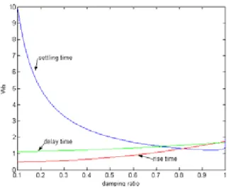
Fig. 3.6(a) The relation between ω_n and ξ when t_s =12, t_d =2and t_r =4

(29)

Fig. 3.6(c) The relation between ω_n and ξ when t_s =7, t_d =1and t_r =2

Fig. 3.6(d) The output controlled and uncontrolled unstable System 2

Table 3.6 ITAE of unstable System 1 and System 2 according to possible ξand ωncombination

ITAE 1 -5 10 2.4593× 0.0012 ξ 0.52 0.82 n ω 1.4 1 ITAE 2 -11 10 1.1791× 0.3848 ξ 0.52 0.82 n ω 1.4 1

(30)

Fig. 3.7(a) The relation between ω_n and ξ when t_s =10, t_d =1and t_r =3

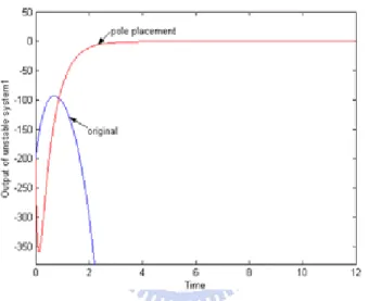
Fig. 3.7(b) The output of controlled and uncontrolled unstable System 1

(31)

Fig. 3.8(a) The relation between ω_n and ξ when t_s =2.5, t_d =0.5and t_r =1

Fig. 3.8(b) The output of controlled and uncontrolled unstable System 1 where ω_n =4 and

98 . 0 = ξ

Fig. 3.8(c) The output of controlled and uncontrolled unstable System 2 where ω_n =4 and

98 . 0 = ξ

(32)

Those design demands will be used also in the following simulations in Chapter 5. From the above simulations, the chose poles of DC motor servo system1 and system2 are s=−380±0.08iand s=−540±0.8i, respectively. The chose poles of unstable system1 and system2 are s=−3±0.3iands =−10±0.08i, respectively.

(33)

CHAPTER 4

NETWORK STABILITY ANALYSIS

The former chapters have mentioned sub-plant systems and their controllers. In this chapter, we will introduce the main idea in this thesis- network control system stability. We want to find out a transmission error- the difference between present state and former control state – to act as a kind of control standard. All the control signals are changed according to this standard. The standard is also a kind of boundary. As long as the transmission error of present state is within the derived boundary, the system stability and network resources can be guaranteed.

Fig 4.1 Transmission error bound

4.1 Lyapunov Stability Theory

It is very easy to check whether a linear system is stable by computing its eigenvalues and checking their real parts. Obviously, adding network system criteria to original linear system makes very big differences on stability and system performances. The stability is no longer guaranteed and neither do the performance of the original designed controller. Therefore, Lyapunov stability theory provides us another option to deal with the stability problems in advance. The Lyapunov stability theory we mention here, actually, is the second method of Lyapunov theory which is also called the direct method of Lyapunov. In the following discussion, we will use the phrase “Lyapunov theory” instead.

Lyapunov theory allows us to determine the stability of a system without explicitly integrating the differential equation (2-13). The method is a generalization of the idea that if there is some form of “measure energy” in a system, then we can study the rate of change of the energy of the system to ascertain stability. To make this precise, we need to define exactly what one means by “measure energy.” Before we define the “measure energy”, we will present the general form of Lyapunov equation. Let Q>0 be a

(34)

positive definite symmetric matrix and let P denote the unique positive symmetric solution of Q A P P AT ⋅ + ⋅ =− (4-1) where is system matrix of , and let be a non-negative function with derivative along the trajectories of the system. The is defined as

A x&= Ax V( tx, ) V& V( tx, ) x P x t x V( , )= T⋅ ⋅ (4-2) where P is the solution of Lyapunov equation (4-1). From equation (4-2), we can view as a kind of energy form of the system. The function V can serve as a measure for the length of the vector x. If, in addition, , we see that is a decreasing function of t along any trajectory . This suggests that the quantity

and hence the vector tends to zero as V 0 > Q V&( tx, ) ) (t x ) , ( tx

V& x(t) t→∞, and hence that is

stable.

Ax

x&=

In other word, as long as has been proved, the stability of system is then maintained. The relation between Lyapunov equation and (4-2) can be shown as follows: 0 < V& x P x Px x

V& = &T + T & (4-3) If taking (2-13) into (4-3) and with pole placement control input in (3-1), we got

(4-4) x F B A P x Px F B A x V& = T( − ⋅ )T + T ( − ⋅ ) To make V&<0, and the inequality is given by

0 ) ( ) (A−B⋅F Px+x P A−B⋅F x< xT T T (4-5) By rearranging (4-5), we have 0 )] ( ) [(A−B⋅F P+P A−B⋅F x< xT T (4-6) Inequality (4-6) sustains if the condition (4-7) holds.

Q F B A P P F B A− ⋅ )T⋅ + ⋅( − ⋅ )=− ( (4-7) Equation (4-7) is the Lyapunov equation of system (2-13).

4.2 Modified Lyapunov Stability with Network Conditions

In conventional controller design, it is very natural to stabilize an unstable system. The condition of V& <0 for all x≠0 is always required. The main idea of Lyapunov

(35)

theory is also to promise stability of control system. However, there are some mechanical systems that are already stable without compensation. DC motors are one of those examples. In this situation, it is meaningless to discuss whether . Therefore, in this section, modified stability standards will be discussed.

0 < V& V K V&<− ⋅ (4-8) Instead of proving to satisfy the stability demands of the system, inequality (4-8) shows more emphases on the decay rate of the system. We now focus our attention on the better performances of control system but not only the stability. The corresponding modified Lyapunov equation becomes

0 < V& Q P K F B A P P F B A− ⋅ )T ⋅ + ⋅( − ⋅ )+ ⋅ =− ( (4-9)

This result will be used in the proofs of Proposition 1.

All of the discussion of Lyapunov stability theory does not yet consider network criteria. To introduce network condition in our discussion, we first replace control input (2-13) with (2-15). Equation (4-4) becomes

)) ( ) ( ( ) ( ) ( )) ( ) ( (A x t B F x t_k TPx t x t TP A x t B F x t_k V& = ⋅ − ⋅ ⋅ + ⋅ − ⋅ ⋅ (4-10)

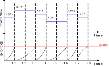
where , and represents the initial time. Considering the inherent physical problem of network systems, the control input signals are not always available, and the period during every access time of the controller is not constant. In order to maintain system performances, a bounded error will be defined in the following proposition. Fig. 4.2 shows the relation between transmission error bound and control state.

t t t₀ < _k < t₀ T 1 T 2 T 3 T 4 T 5 T 6 T 7 T 8 Co nt ro l St a te || x( t) -x (t k )|| T i m e X ( t 1 ) X ( t 2 ) X ( t 4 ) X ( t 5 ) X ( t 6 ) | | e ( t ) | | T i m e X ( t 3 )

(36)

Proposition 1:

Letx∈Rn,Q,P∈Rn×n, B∈Rn, and F∈R1×n where are positive definite matrices.

P Q,

B is the system matrix in (2-15), and F is the state feedback gain. P is

the unique solution of modified Lyapunov equation (4-9) according to specific . If the error is limited as

Q 1 min( ) ( ) 2 1 ) (t < ⋅ Q x t ⋅ PBF − e λ (4-11) where t₀ <t_k <t, and e(t)= x(t)−x(t_k). The system can be guaranteed to have Lyapunov stability of

KV

V& <− (4-12) where is given in (4-2), and system model is V(x,t)

) ( ) ( ) (t A x t B u tk x& = ⋅ + ⋅ Proof: x P x Px x

V& = &T + T &

Form (4-10), we have ( ( ) ( )) ( ) ( ) ( ( ) ( k)) T T k Px t x t P Ax t BFx t t BFx t Ax V& = − + − )) ( ) ( ( ) ( 2xT t P Ax t −BFx t_k = we assume that 1 min( ) 2 1 ) (t < Q x ⋅ PBF − e λ

where , and e(t)=x(t)−x(t_k) Q is identity matrix in (4-7).

x Q x t e PBF xT T ( ) 2 1 ) ( < ⋅ λ_min ⋅ ⋅ 2 min( ) 2 1 ) (t Q x e PBF xT ⋅ ⋅ < λ

(37)

2 2 1 ) (t Q x e PBF xT ⋅ ⋅ < Qx x t e PBF xT T 2 1 ) ( < ⋅ ⋅ 0 ) ( 2 ) (−Q x+ x ⋅ PBF ⋅ e t < xT T It is obvious that ) ( 2 ) ( ) ( 2 ) ( Q x x PBFet x Q x x PBF e t xT − + T ≤ T − + T ⋅ ⋅ If 0 ) ( 2 ) (−Q x+ x ⋅ PBF ⋅ e t < xT T Then, 0 ) ( 2 ) (−Q x+ x PBFe t < xT T Taking substituting (4-9) into above inequality we have

0 )] ( ) ( [ ) ( 2 ) ( } ) ( ) ){( ( − T + − + + T − _k < T t x t x PBF t x t x KP BF A P P BF A t x 0 2 2 )] ( [ 2xTP Ax−BFxt_k +K⋅xTPx+ xTPBFx− xTPBFx< ) ( ) ( )) ( ) ( ( ) ( 2xT t P Ax t −BFx t_k <−K⋅xT t Px t

We substitute V&and V into above inequality, then we have

V K V&<− ⋅

▓

Lemma 1:

Consider a linear time-invariant system in (2-13). Letx∈Rn,Q,P∈Rn×n, B∈Rn, and F∈R1×n where Q,Pare positive definite matrices. B is the system matrix in

(2-15), and F is the state feedback gain. P is the unique solution of modified

(38)

1 1 min( )[ ( ) ] ( ) 2 1 ) (t < Q M +A− I −M BF x t ⋅ PBF − e λ _k (4-13)

where _M =_eA(t−tk), and system model is

) ( ) ( ) (t A x t B u tk x& = ⋅ + ⋅ Proof:

The trajectory expression of x(t) with t₀ =t_k is given as

∫

− − ₊ = t t t A k t t A k k _x _t _e _Bu _d e t x( ) ( ) ( ) ( τ) (τ) τ

Taking (3-1) with t₀ =t_kinto above equation, we have

∫

− − ₋ = t t k t A k t t A k k _x _t _e _BFx _t _d e t x( ) ( ) ( ) ( τ) ( ) τ ( ) ( ) ( k) t t A At k t t A t BFx d e e t x e k k

∫

− − ₋ = τ τ ( ) ( ) ( 1 t ) ( _k) t A At k t t A t BFx e A e t x e k k = − − − ₋ ₋ = τ τ [ ( ) 1( ) ] ( k) At At At t t A t x BF e e A e e −k + − − − − k = =[eA(t−tk) +eAtA−1e−At(I −eA(t−tk))BF]x(t_k) [ ( ) 1( ( )) ] ( k) t t A t t A t x BF e I A e −k + − − −k = =[M +A−1(I −M)BF]x(t_k) (4-14)

where _M =_eA(t−tk). If take (4-14) into Proposition 1, the inequality became

1 1 min( )[ ( ) ] ( ) 2 1 ) (t < Q M +A− I−M BF x t ⋅ PBF − e λ _k ▓ Proposition 1 describes the error bound [x(t)−x(tk)] of a local plant. As long as

(39)

the error bound is within the proved range, the system can have better performance than the original system, and the results will be shown in Chapter 5 in simulations.

Lemma 2 will introduce network delays. It is an extent manifestation of Proposition 1. Another formation of bounds will be shown in the following proposition. The system state space is

) (t

Bu Ax x& = +

where the input control is given as follows

) ( )

(t =−Fx tk −τ

u

where .Fig. 4.3 shows the relation between control states and error bounds with time delays.

1 + < < _k k t t t T 1 T 2 T 3 T 4 T 5 T 6 T 7 T 8 Contr o l S tat e ||x( t)-x (t k) || X ( t 1 ) X ( t 2 ) X ( t 4 ) X ( t 5 ) X ( t 6 ) | | e ( t ) | | T i m e d e l a y T i m e X ( t 3 )

Fig. 4.3 Transmission error bound and control states of NCS with delays

Lemma 2:

Consider a linear time-invariant system in (2-13). Letx∈Rn,Q,P∈Rn×n, B∈Rn, and F∈R1×n where Q,Pare positive definite matrices. B is the system matrix in

(2-15), and F is the state feedback gain. P is the unique solution of modified

Lyapunov equation (4-9) according to specific . If the delayed control state is limited as given Q 1 1 min( )[ ( ) ] ( ) 2 1 ) ( ) (t −x t − < Q M +A− I−M BF x t ⋅ PBF − x k τ λ k

(40)

guaranteed to have Lyapunov stability of (4-12) where is (4-2), and system model is V ) ( ) ( ) (t = A⋅x t +B⋅u t_k −τ x& Proof: x P x Px x

V& = &T + T &

Adopted form (4-10) where the input signals are delayed states, we have )) ( ) ( ( ) ( ) ( )) ( ) ( ( − −τ + − −τ = T T _k k Px t x t P Ax t BFx t t BFx t Ax V& )) ( ) ( ( ) ( 2 − −τ = k T t BFx t Ax P t x

where t_k₋₁ <t_k −τ <t . We first assume that

1 1 min( )[ ( ) ] ( ) 2 1 ) ( ) (t −x t − < Q M +A− I−M BF x t ⋅ PBF − x k τ λ k

where we substitute (4-14) into above inequality

1 min( ) 2 1 ) ( ) (t −x t − < Q x ⋅ PBF − x k τ λ x Q x t x t x PBF xT _k T ( ) 2 1 ) ( ) ( − −τ < λ_min ⋅ Qx x t x t x PBF x k T T 2 1 ) ( ) ( − − < ⋅ ⋅ τ It is obvious that ) ( ) ( 2 ) ( )] ( ) ( [ 2 ) (− + − −τ ≤ − + ⋅ ⋅ − k −τ T T k T T t x t x PBF x x Q x t x t x PBF x x Q x If 0 ) ( ) ( 2 ) (− + ⋅ ⋅ − k −τ < T T t x t x PBF x x Q x Then,

(41)

0 )] ( ) ( [ 2 ) (− + T − _k −τ < T t x t x PBF x x Q x

Taking substituting (4-9) into above inequality we have

0 )] ( ) ( [ ) ( 2 ) ( } ) ( ) ){( ( − T + − + + T − _k −τ < T t x t x PBF t x t x KP BF A P P BF A t x 0 2 2 )] ( [ 2xTP Ax−BFx t_k −τ +K⋅xTPx+ xTPBFx− xTPBFx< 0 ) ( ) ( )) ( ) ( ( ) ( 2x t P Ax t −BFx tk − +K⋅xT t Px t < T τ ) ( ) ( )) ( ) ( ( ) ( 2xT t P Ax t −BFx t_k −τ <−K⋅xT t Px t

We substitute V&and V into above inequality, then we have

V K V&<− ⋅

▓ Lemma 2 is actually an extension of Proposition1. In the results of Lemma 2, the effect caused by fixed delay τ is described by β(t).

(42)

4.3 Simulations

The following simulations are demonstrated by speed control of two different DC

motor servo systems and two randomly selected different linear unstable systems. The detailed parameters of DC motor servo system and unstable systems are given in Table 3.2 and as follows.

) ( ) ( ) (t A x t B u t x& = ⋅ + ⋅ where _⎥ and . ⎦ ⎤ ⎢ ⎣ ⎡ − − − = 7 . 0 2 8 . 0 2 A _⎥ ⎦ ⎤ ⎢ ⎣ ⎡ = 1 1 B

) ( ) ( ) (t A x t B u t x& = ⋅ + ⋅ where _⎥ and . ⎦ ⎤ ⎢ ⎣ ⎡ = 10 3 1 1 A _⎥ ⎦ ⎤ ⎢ ⎣ ⎡ = 2 1 B

The controlling block diagram is shown in Fig. 4.4.

Sub-system1 Central Controller

-Sub-system2

-. . . u1 u2 states1 states2

(43)

4.3.1 Network Control System without Delay

The following simulations will demonstrate the controlled results of systems considering transmission error. All the controlling conditions and system details are the same as mentioned in section 4.3. The most different part is that innate characteristics- transmission error- of NCSs are considered. However, the network-induced delays are not involved in. In practical NCS, not every feedback states are available during every sampling time, and therefore the control input signal might not be compatible to present states and is calculated according to some states before. Lyapunov stability theory is adopted when deriving the transmission error bound in Chapter 4. The control input signal is changed based on transmission bound. Finally, the endurable error is within 0.001.

(1)DC motor systems

Fig. 4.5(a) The angular velocity of transition error controlled and uncontrolled system of System1

(44)

Fig. 4.5(c) The controlled frequencies of DC motor ststem1 and system2 (2)Unstable systems 0 1 2 3 4 5 6 7 8 -400 -350 -300 -250 -200 -150 -100 -50 0 50 O u tp ut o f u n st ab le syst e m 1 orginal controlled system

Fig. 4.6(a) The output of transition error controlled and uncontrolled system of Unstable system1

0 0.2 0.4 0.6 0.8 1 1.2 1.4 1.6 1.8 2 -200 -180 -160 -140 -120 -100 -80 -60 -40 -20 0 20 O u tp ut o f u n st ab le syst e m 2 i i l cotrolled system

(45)

Fig. 4.6(c) The controlled frequencies of Unstable sytem1 and system2

The same pole placement results of section 4.3 are also used in this section. Fig.

4.5 are, comparing with single plant control, not so ideal in transient performances especially in delay time and rise time. On the other hand, the controlled frequencies deserve to be mentioned. For DC motor servo systems, the frequencies are 5000/25000 times at most. Unstable systems are 25000/400000 times. The controlled frequencies are system depending. Even the worse case in DC motor system, nine tenth network usage is saved and about three fourth for unstable system.

4.3.2 Network Control System with Delay

In this section, all the controlling conditions and system details are the same as mentioned in section 4.3.1. An overall NCS with constant delays is presented. The constant delay adopted is 44.4 μsec.

(1)DC motor systems

Fig. 4.7(a) The angular velocity of transition error controlled with delays and uncontrolled system of System1

(46)

Fig. 4.7(b) The angular velocity of transition error controlled with delays and uncontrolled system of System2

Fig. 4.7(c) The controlled frequencies of DC motor ststem1 and system2 with delays

(2)Unstable systems 0 1 2 3 4 5 6 7 8 -200 -150 -100 -50 0 O u tp ut o f un s ta b le s yst e m 1 original controlled system

Fig. 4.8(a) The output of transition error controlled with delays and uncontrolled system of Unstable system1

(47)

0 1 2 3 4 5 6 7 8 -400 -350 -300 -250 -200 -150 -100 -50 0 50 O u tp u t o f u n s ta b le s y s te m2 original controlled system

Fig. 4.8(b) The output of transition error controlled with delays and uncontrolled system of Unstable system2

Fig. 4.8(c) The controlled frequencies of Unstable sytem1 and system2 with delays

The simulations show that adding of delay decreases system efficient a lot. Taking DC motor systems for example, only three fourth network resources are saved and the unstable systems are even worse. Although the stability is promised in both system types, the advanced performances are not always guaranteed. Therefore, it is very important to make sure the demands of NCS before design one. If the demands are only focus on system stability, the design is good enough. But if designers are focus on other system performances, it needs more compensating and amending.

(48)

CHAPTER 5 CONCLUSIONS

5.1 Remark Conclusions

In this thesis an error bound concept is provided to function as a switching standard of networked control systems. The system needs control only when the error bound is over the calculated value which is closely related to present state or former available state. The standard is quite reasonable. Through network systems, many unpredictable situations will inevitably appear in the systems such as network induced time delay and packet losses. Besides, there is also some other algorithm problems need to be considered, for example, scheduling or package dropping. Any of these tasks put great deal of influences on the NCS performance and stability.

The lesser the unnecessary accesses to the network the more efficient the NCS is. The concept of error bound could maintain this condition. Local sensors can sieve out the error bound of every state and send out control demands to the central controller and then the central controller can send control signal to the local actuators. It is no need for central controller to send control signal to every node for every state which is impossible for practical layer. In small local NCS with few nodes, the achievements are not conspicuous, but the effect would be very noticeable in large NCS. For example, if one node covers only

10

1 _{lesser network usage than before, a NCS with 100 nodes}

could save 10

9 _{usage of the network and is very flexible for another possible 90 more} nodes to enlarge the original 100 nodes NCS. This means the original NCS could have around 90% in growth. The influences of the error bound are very useful and ideal.

The simulations of switched systems illustrate the most ideal situations in NCS that is merely possible in practical realization. It means every feedback state is available, and also fixed time slots are set for specific nodes without considering the fact that the feedback states of the node might not be available during the specific time slots. The other simulations are modeling actual network criteria without delays and with delays. The mentioned turn, , is sometimes called transmission error[9]. The simulation results of those two situations demonstrate the influences network part brought to the NCS. Comparing with ideal situations, the performances are not so good although the stability is still promised.

) (t

(49)

5.2 Future Work

The detailed relation between system performance and stability is not so clear and definitely so far in the discussion. Different sub-plant may have different demands in design and their limitations are quite diverse, too. We use pole placement methodology, in this thesis, to maintain DC motor performance. For unstable systems, the most crucial problem lays on stability which is much more important than system transient performance comparing with DC motors.

Pole placement methodology is good at controlling the transient states of a system, but there are following limitations. There are always limited bounds for the locations of poles. The design methodology mentioned in this thesis, is just objective orientation ; not intending to find exactly pole locations. For more complex and larger systems, other controller design might be better and powerful choices such as optimal control, H infinity or robust control. It is also possible to design a compensation controller for the pole placement controller without thoroughly changing original controller.

There are many other more complex problems appearing in real NCSs. It would be a very complete discussion if those criteria could be transformed in to mathematical expression and be considered in the NCSs. Every condition has different impact on system stability or performance. If we could consider more practical situations, the derived consequences could be more persuasive and more flexible.

There are also some discussions about the modified Lyapunov equation. According to (4-8), the modified Lyapunov equation is shown in (4-9). However, it is not for sure that whether the equation has a solution. More mathematical proof needs to be continued and discussed.

(50)

REFERENCE

[1] Y. Halevi and A. Ray, “Integrated communication and control systems: “Part I—Analysis,” J. Dynamic Syst., Measure. Contr., vol. 110, pp. 367-373, Dec., 1988. [2] J. Nilsson, “Real-time control systems with delays,” Ph.D. dissertation, Dept. of Automatic Control, Lund Institute of Technology, Lund, Sweden, January, 1998.

[3] G.C. Walsh, H. Ye, and L. Bushnell, “Stability analysis of networked control systems,” in Proc. Amer. Control Conf. , pp. 2876-2880, San Diego, CA, June 1999. [4] M.S. Branicky, S.M. Phillips, and W. Zhang, “Stability of networked control systems: Explicit analysis of delay,” in Proc. Amer. Control Conf, pp. 2352-2357, Chicago, IL, June 2000.

[5]Electro-Craft Corporation, “DC motors, speed controls, servo systems: an engineering handbook,” Pergamon press, Reading, 1972, 3rd edition.

[6] B. C. Kuo, Automatic control systems, John Wiley & sons, Reading, 1993, 6th edition.

[7]L. Xie, J. M. Zhang, and S. Q. Wang, “Stability analysis of networked control system,” Proceedings of the First International Conference on MLC, Beijing, 4-5 Nov. 2002.

[8]N. B. Almutairi, M. Y. Chow, “PI Parameterization Using Adaptive Fuzzy Modulation (AFM) for Network Control Systems – Part I: Partial Adaptation,” for possible presentation at IECON 2002,pp3152-3157, Sevilla, Spain, 2002.

[9]W. Zhang, “Stability Analysis of Network Control Systems,” Ph.D. dissertation, Dept. of Electrical Engineering and Computer Science, Case Western Reserve University, Aug., 2001.

[10]J. Ackermann, “Robust Control: Systems with Uncertain Physical Parameters,” Springer-Verlag, New York, 1993.

[11]K. J. Astrom, and B. Wittenmark, “Computer-Controlled Systems: Theory and Design,” 3rd. Edition, Prentice-Hall, Upper Saddle River, NJ, 1997.

[12]B. R. Barmish, “New Tools for Robustness of Linear Systems,” Macmillan Publishing Co., New York, 1994.

[13]H. L. Trentelman, A. A. Stoorvogel, and M. L. J. Huatus, “Control Theory for Linear Systems,” Springer-Verlag, London limited, 2001.