應用於直流馬達速度控制之灰預測器

全文

(1)國立交通大學電機與控制工程學系碩士論文. 應用於直流馬達速度控制之灰預測器 Grey Predictor Applied to Speed Control of DC Motor. 研究生：梁智淵指導教授：陳永平教授. 中華民國九十三年六月.

(2) 應用於直流馬達速度控制之灰預測器 Grey Predictor Applied to Speed Control of DC Motor. 研究生：梁智淵. Student：Chih-Yuan Liang. 指導教授：陳永平. Advisor：Yon-Ping Chen. 國電. 機. 立與. 交控. 碩. 通制. 士. 大工. 論. 學程. 學. 系. 文. A Thesis Submitted to Department of Electrical and Control Engineering College of Electrical Engineering and Computer Science National Chiao Tung University in partial Fulfillment of the Requirements for the Degree of Master in Electrical and Control Engineering June 2004 Hsinchu, Taiwan, Republic of China. 中華民國九十三年六月. 2.

(3) 應用於直流馬達速度控制之灰預測器. 學生：梁智淵. 指導教授：陳永平博士. 國立交通大學電機與控制工程研究所碩士班. 摘. 要. 本篇論文主要在驗證灰預測器在雜訊預測以及應用於直流馬達速度控制上的效能。在此我們採取順滑模態控制來做直流馬達的速度控制，因其對消除匹配式雜訊有很好的效果；但是傳統的順滑模態控制需在匹配式雜訊的上限值已知的前提下才能有如此好的性能。然而，雜訊的上限值是很難準確的量測或估算出來的，而要是雜訊的上限值估算得不準的話，整個系統就會產生不穩定的現象。可想而知，若是每一點的雜訊大小都能預測得到的話，那我們就可以直接對雜訊作處理而不必理會整個雜訊的上限值了。在論文中我們以多種不同組合的雜訊來做灰預測器的效能評估，並且與線性迴歸的方法作比較，結果顯示灰預測器對於較低頻或較沒有劇烈變化的雜訊有蠻好的效果。同樣地，在應用到順滑模態控制方面的模擬結果也顯示出這樣的結合確實可以解決估算雜訊上限值的問題。. i.

(4) Grey Predictor Applied to Speed Control of DC Motor. student：Chih-Yuan Liang. Advisors：Dr. Yon-Ping Chen. Institute of Electrical and Control Engineering National Chiao Tung University. ABSTRACT. This thesis verifies the efficiencies of grey predictor on the prediction of the disturbances and the application to speed control of DC motor. Sliding-mode control is chosen here for speed control of DC motor because of its robustness of eliminating the matched disturbances. The traditional sliding-mode control has such property with the hypothesis that the upper bound of the disturbances is known. However, the upper bound of the disturbance is difficult to be measured or estimated exactly, and the system would be unstable if the upper bound is not well estimated. It is obvious that if the value of the disturbances could be predicted well, the upper bound would not be necessary information any more. In the thesis, the performances of grey predictor are evaluated with several distinct disturbances and compared with the performances of linear regression method. The simulation results show that grey predictor has well performances for the disturbances with lower frequency or less rapid variations, and it can solve the problem of estimating the upper bound of the disturbances.. ii.

(5) Acknowledgement. 本論文能順利完成，首先得感謝指導老師陳永平教授這兩年來孜孜不倦的辛勤教導，除了在課業方面的解惑之外，老師也很注重學生的學習態度、研究方法以及在語文能力上的培養；因此，也讓我在這些方面有了相當的成長，謹在此向老師致上最高的謝意。此外，也要感謝張浚林學長在繁忙的工作之餘還抽空為我解答研究上所遇到的的種種問題，並不時地給予我鼓勵，在此獻上最誠摯的謝意；最後，感謝口試委員梁耀文老師以及張浚林學長提供寶貴意見，使得本論文能更臻於完善。同時，也要感謝可變結構控制實驗室的所有所有人員，包括克聰學長、天德學長、豐裕學長、建峰學長、豐洲學長、培瑄、依娜、翰宏、倉鴻、世宏以及所有的學弟們對我的照顧與陪伴，讓我在實驗室的研究生活充滿溫馨與快樂。另外，還要感謝我的室友翰宏和平修，他們在我遇到挫折時一直在一旁幫我打氣，使我不至於被挫敗打倒；最後，要感謝我的家人對我的照顧，有他們在背後的全力支持，我才能夠不斷的勇往直前。謹以此篇論文獻給所有關心我、照顧我的人。. 梁智淵 2004.6.28. iii.

(6) Contents Chinese Abstract…………………………………………………………….. i English Abstract………………………………………………………………ii Acknowledgement............................................................................................iii Contents………………………………………………………………………iv List of Figures……………………………………………………………….. v. Chapter 1. Introduction…………………………………………………...01. Chapter 2 System Descriptions 2.1 Mathematical Model………………………………………………….. 04 2.2 Software and Hardware Architecture………………………………….06 Chapter 3 Grey Prediction 3.1 Grey Theory…………………………………………………………... 14 3.2 Grey Prediction……………………………………………………….. 16 Chapter 4 Controller Design 4.1 Introduction of Sliding-Mode Control………………………………... 24 4.2 Conventional Sliding-Mode Controller Design………………………. 27 4.3 Sliding-Mode Controller Design Combined with Grey Prediction……29 Chapter 5 Simulation Results……………………………………………... 33 Chapter 6 Conclusions……………………………………………………... 55 Reference…………………………………………………………………….56. iv.

(7) List of Figures. Figure 2.1 – DC motor rotation system............................................................04 Figure 2.2 – ‘set path’ function window ..........................................................09 Figure 2.3 – The xPC target setup menu..........................................................10 Figure 2.4 – Simulink block diagram...............................................................11 Figure 2.5 – The xPC target scope window .....................................................12 Figure 3.1 – The block diagram of grey prediction..........................................19 Figure 3.2 – Results of the grey prediction ......................................................21 Figure 4.1 – The system’s behavior within the sliding layer ...........................24 Figure 5.1(a) – The predicted result of GM(1,1)..............................................35 Figure 5.1(b) – The predicted result of linear regression.................................36 Figure 5.1(c) – The predictive error of GM(1,1) and linear regression ...........36 Figure 5.2(a) – The predicted result of GM(1,1)..............................................37 Figure 5.2(b) – The predicted result of linear regression.................................37 Figure 5.2(c) – The predictive error of GM(1,1) and linear regression ...........38 Figure 5.3(a) – The predicted result of GM(1,1)..............................................38 Figure 5.3(b) – The predicted result of linear regression.................................39 Figure 5.3(c) – The predictive error of GM(1,1) and linear regression ...........39 Figure 5.4(a) – The predicted result of GM(1,1)..............................................40 Figure 5.4(b) – The predicted result of linear regression.................................40 Figure 5.4(c) – The predictive error of GM(1,1) and linear regression ...........41 Figure 5.5(a) – The predicted result of GM(1,1)..............................................41 Figure 5.5(b) – The predicted result of linear regression.................................42 Figure 5.5(c) – The predictive error of GM(1,1) and linear regression ...........42 v.

(8) Figure 5.6(a) – The predicted results of GM(1,1) and PGM(2,1)....................43 Figure 5.6(b) – The predictive error of GM(1,1) and PGM(2,1) .....................44 Figure 5.7(a) – The predicted results of GM(1,1) and PGM(2,1)....................44 Figure 5.7(b) – The predictive error of GM(1,1) and PGM(2,1) .....................45 Figure 5.8(a) – The predicted results of GM(1,1) and PGM(2,1)....................45 Figure 5.8(b) – The predictive error of GM(1,1) and PGM(2,1) .....................46 Figure 5.9(a) – The predicted results of GM(1,1) and PGM(2,1)....................46 Figure 5.9(b) – The predictive error of GM(1,1) and PGM(2,1) .....................47 Figure 5.10(a) – The predicted results of GM(1,1) and PGM(2,1)..................47 Figure 5.10(b) – The predictive error of GM(1,1) and PGM(2,1) ...................48 Figure 5.11(a) – The simulation result of the novel sliding mode control.......49 Figure 5.11(b) – The simulation result of traditional sliding mode control.....50 Figure 5.12(a) – The simulation result of the novel sliding mode control.......50 Figure 5.12(b) – The simulation result of traditional sliding mode control.....51 Figure 5.13(a) – The simulation result of the novel sliding mode control.......51 Figure 5.13(b) – The simulation result of traditional sliding mode control.....52 Figure 5.14(a) – The simulation result of the novel sliding mode control.......52 Figure 5.14(b) – The simulation result of traditional sliding mode control.....53 Figure 5.15(a) – The simulation result of the novel sliding mode control.......53 Figure 5.15(b) – The simulation result of traditional sliding mode control.....54. vi.

(9) Chapter 1 Introduction. The presence of disturbances is an inevitable feature of control systems, no matter linear or nonlinear systems, and the disturbances would cause unwanted effects on the system’s performance. Many investigators have proposed diverse methods to deal with the disturbances, such as the disturbance accommodation control (DAC) [1] and the internal-model-based repetitive control [2]. The basic idea of DAC is to model the disturbance, augment its state equations to the system state equations, and then reconstruct the states of this augmented system for use in a controller that minimizes the effects of the disturbance. For this control scheme to work, the disturbances must be of known waveform type, such as a step function, ramp function, and so forth. It is actually speaking that, however, the disturbances in physical systems are very difficult to model. As for the internal-model-based repetitive control, it could deal with repeatable disturbances but amplifying non-repeatable disturbances, which are at frequencies between those of the repeatable disturbances. Due to these drawbacks, they are not so practicable and the sliding-mode control is chosen here because of its robustness for system’s parametric uncertainties and the elimination of matched external disturbances.. 1.

(10) Disturbance suppression and adaptation to internal system parameter variations are important as well as the command input response characteristics in designing control systems. In order to suppress the disturbance and to improve the robustness, high-gain controllers are employed in general. However, it is well known that in controlling elastic electro-mechanical systems, high gain controllers can cause resonance easily [3]. The traditional sliding-mode control is one kind of high gain control since the upper bound of the disturbances are often over-estimated. It might be argued that if the disturbances can be estimated, the control problems of the systems with disturbances may become easier to solve. Many investigators have paid their attentions to disturbance observers or estimators. Nevertheless, most of them need a large amount of data or the complicated calculation to do the observation or estimation. A new approach adopting grey theory is proposed in this thesis to not only estimate the disturbances but also predict the disturbances, and it can be called as grey predictor. Besides, the simulation of the grey predictor applied to speed control of DC motor combined with sliding-mode control will be presented. The rest of this thesis is organized as follows: following the introduction, the system descriptions, including the mathematical model of the system and system’s software and hardware architectures, will be introduced in Chapter 2. In Chapter 3, the concepts of grey theory and the derivation of grey prediction model, GM(1,1), will. 2.

(11) be shown. The next chapter contains the brief introduction of the sliding-mode control, the traditional sliding-mode controller design, and design of the sliding-mode controller incorporated with grey prediction. In Chapter 5, some computer simulations and comparisons will be given to demonstrate the effectiveness of the proposed method, and finally, some conclusions are drawn in Chapter 6.. 3.

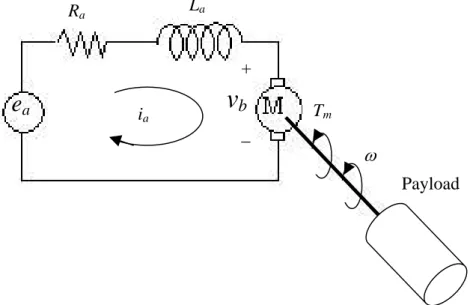
(12) Chapter 2 System Descriptions System descriptions will be introduced in Chapter 2. First, the mathematical model of a DC motor will be shown in Section 2.1 and the general diagram of the rotation system of a DC motor mounted with payload is shown in Figure 2.1. Then, the software and hardware architectures will be introduced in Section 2.2. La. Ra. +. ea. ia. vb. Tm. −. ω Payload. Fig. 2.1 DC motor rotation system. 2.1 Mathematical Model The dynamic equation of a DC motor, schematically depicted in Figure 2.1, is generally expressed as La. dia + Ra i a + vb = e a dt. (2.1). 4.

(13) where La and Ra are the inductance and resistance of armature, ia and ea represent the current. through. and. the. voltage. across. the. armature,. and. vb. is. the. back-electromotive force. Since vb is proportional to the angular velocity of motor ω as vb = K b ω and La is negligible, (2.1) can be further modified as Ra i a + K b ω = e a. (2.2). Besides, the generated torque of the motor Tm is known as Tm = K t ia. (2.3). which means Tm is proportional to the armature current ia with constant coefficient Kt. By rearranging (2.2) and (2.3), we have Ra. Tm + K b ω = ea Kt. (2.4). When a payload is mounted to the motor as shown in Figure 2.1, the rotational differential equation can be displayed as. Τ m = ( J m + J )ω& + ( Dm + D)ω + τ c. (2.5). where J m and Dm are the motor’s inertia and damping ratio, J represents the rotational inertia of payload, D ω and τ c are respectively the viscous and coulomb friction. Substituting (2.5) into (2.4), we can get Ra [( J m + J )ω& + ( Dm + D)ω + τ c )] + K b ω = ea Kt. (2.6). Since ( Dm + D)ω + τ c consists of damping and friction which are commonly hard to exactly estimated, these terms will be treated as uncertainties or disturbances, denoted. 5.

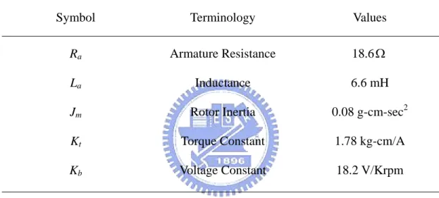
(14) as d = ( Dm + D)ω + τ c . Therefore, (2.6) can be rearranged as Ra [( J m + J )ω& + d ] + K b ω = ea Kt. (2.7). To describe the system as a state equation, let state variable x = ω , control input u = ea , then, (2.7) can be expressed as x& = Ax + Bu + Bd1. where A = −. (2.8). Kt Kb Kt , B= , and d1 = − d . After deriving the Ra ( J m + J ) Ra ( J m + J ). system’s dynamic equation, the system’s software and hardware architectures would be introduced in the next section.. 2.2 Software and Hardware Architectures The parameters of the DC motor are listed in Table 1. The control platform is a PC-based system, which is constructed under xPC Target environment and consists of a master computer and a slave computer with the communication protocol of RS-232 or Ethernet. This PC-based system is called the xPC system here for convenient. The xPC Target, a product of The MathWorks Company, is developed to operate with the Real-Time Workshop in MATLAB software. The xPC Target is a host-target PC solution for prototyping, testing, and deploying real-time systems. In this environment, the user can use MATLAB with Simulink in the master computer to create models. 6.

(15) using Simulink blocks and run simulations to verify whether the controller design is OK or not. Once the simulation results represent as the desired performances, the user can transmit the program code generated by Real-Time Workshop to the slave computer, and run the generated code in the slave computer in real time.. Table 1. Parameters of the DC motor Symbol. Terminology. Values. Ra. Armature Resistance. 18.6 Ω. La. Inductance. 6.6 mH. Jm. Rotor Inertia. 0.08 g-cm-sec2. Kt. Torque Constant. 1.78 kg-cm/A. Kb. Voltage Constant. 18.2 V/Krpm. The MATLAB 6.5 software compiled by Visual C program is installed in the master computer. As for the slave computer, it only needs to be installed with the xPC-MC240 I/O card developed by The Terasoft Incorporated Company and the Advantech1753 LAN card, a specific LAN card. The xPC-MC240 I/O card is integrated with the PLX9052 chip for PCI control and the TMS320F240 DSP chip, where both chips are communicated through SRAM. Besides, the xPC-MC240 I/O card also contains 16 analog input channels (10-bit ADC, 0~5V), 4 analog output. 7.

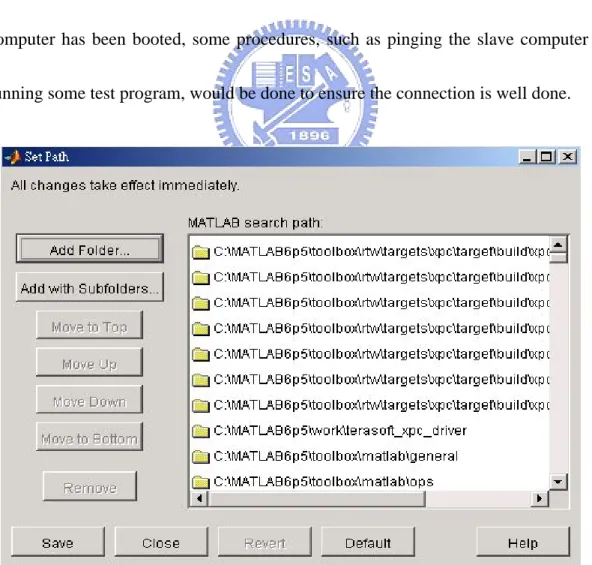
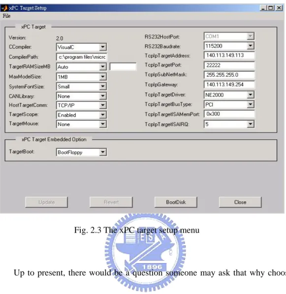
(16) channels (12-bit DAC, ±10V), 16 digital inputs, 16 digital outputs, 6 PWM channels (TTL, 5V), 1 encoder input, and 3 input captures. Among them, the first input capture can also be treated as the QEP input, so the xPC-MC240 I/O card receives signals of the encoder from encoder input pin and the first input capture pin. It should be noted that because of the restriction on the efficiency of the TMS320F240 DSP chip, the maximum sampling frequency is 10KHz; i.e., if the sampling frequency were higher than 10KHz, the A/D conversion time would be insufficient such that the ADC value would be incorrect. Now, let’s see how to install the xPC system. First, there are some additional important working paths should be included in the default working paths menu, which could be added by using the ‘set path’ function in Figure 2.2. The connection between MATLAB and Visual C also has to be constructed so that the xPC system could take the Visual C program as the compiler. Then, the command ’xpcsetup’ would be typed into the command window of MATLAB to pop up the xPC target setup menu, which is displayed in Figure 2.3. There are several relative setup options about the communication protocol and the target computer in the setup menu. The first option is choosing the compiler, such as Visual C, and the blank under the compiler option is the compiler path. The communication protocol between the master and the slave computers is chosen from the ‘HostTargetComm’ option; if RS232 is chosen,. 8.

(17) ‘RS232HostPort’ and ‘RS232Baudrate’ would be determined, on the contrary, if TCP/IP is chosen, ‘TcpIpTargetAddress’, ‘TcpIpTargetPort’, ‘TcpIpSubNetMask’, and ‘TcpIpGateway’ would be assigned. Here, the communication protocol is chosen as TCP/IP because of the higher transmission rate, and the slave computer would be connected to the master computer directly through a LAN cable or indirectly through a hub. When the xPC target setup is finished, the ‘BootDisk’ button would be press down to produce a boot-disk, which contains the specific operating system of the slave computer, and the slave computer would be booted with it. After the slave computer has been booted, some procedures, such as pinging the slave computer or running some test program, would be done to ensure the connection is well done.. Fig. 2.2 ‘set path’ function window. 9.

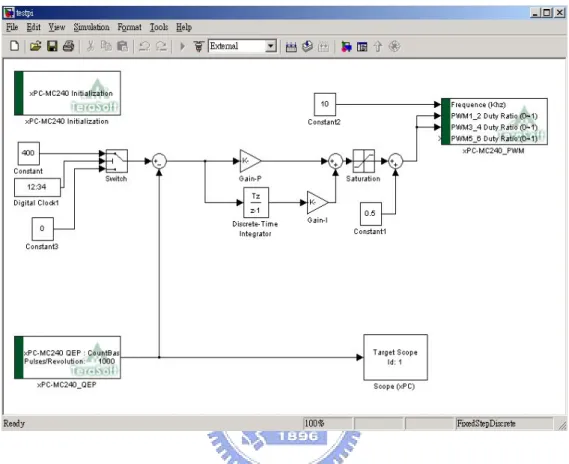
(18) Fig. 2.3 The xPC target setup menu. Up to present, there would be a question someone may ask that why choosing the xPC system even though it requires two computers. It should be known that every function designed in the xPC-MC240 I/O card, such as ADC, DAC, PWM, and so on, has its own module block. Thus, one of the advantages of the xPC system is that the control algorithm could be verified by using block diagram as mentioned before instead of writing the program codes. In other words, the user can do the experiment just by using the general Simulink block incorporated with the individual module block of the xPC-MC240 I/O card to construct the controller block diagram, such as Figure 2.4. Such designed method can solve the problem that something may be. 10.

(19) difficult to be represented by the program codes, and reduce the consuming time of try and error and debugging.. Fig. 2.4. Simulink block diagram. In addition, it is a common phenomenon that students usually have some operative errors or negligence when they are doing the experiments. If the control platform were a single-PC-based system, it would take a large amount of cost when a critical operative error happens. For the xPC system, the hardware is constructed on the slave computer, which doesn’t need to be equipped with so high-level equipments as those in the master computer. Thus, it would not take so much cost as the single-PC-based system does even though a crucial mistake is made. Furthermore,. 11.

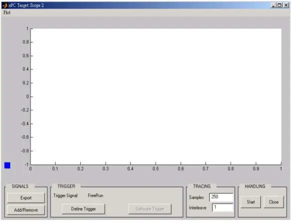
(20) when the user uses the xPC system, the command ‘xpcscope’ could be typed into the command window of MATLAB to pop up the xPC target scope window, Figure 2.5, where the real-time results would be shown. After the xPC target scope window was popped up, the user could add the desired signals whose real-time results would be shown on the scope window, and choose the signals that would be exported. When the desired results have been shown, the user could stop the program, export the results, and then save the numerical results and waveforms.. Fig. 2.5 The xPC target scope window. It is actually speaking that the xPC system is not only a powerful but also an extendable system. It could be applied to several fields, such as mobiles and 12.

(21) navigation controls, industrial automation, robotics and motion controls, and so forth. It also could provide the assistance in the simulations of various operations of the embedded control system, such as system rapid prototyping and hardware-in-the-loop. Except the one-on-one control system, the xPC system also can do the multi-system control as long as the connection could be successfully established, whether one master computer vs. multiple slave computers or multiple master computers vs. one slave computer. Moreover, if the xPC Target Embedded Option were added into the xPC Target environment, it would have stand-alone application, which means that the user can run target applications on the slave computer without connecting to the master computer for deploying the applications.. 13.

(22) Chapter 3 Grey Prediction In the control theory, people usually use the deepness of colors to describe the clearness of the message, for example, Ashby called the object with unknown inner messages a “Black Box”. In general, a system with exactly definite inner messages is called a white system; on the contrary, a system whose inner messages are all unknown is called a black system. However, it is impossible to divide all the systems into just black type or white type, i.e., most systems have both definite and unknown inner messages. Such system may be given a name as grey system, and the grey theory is evolved to deal with the relative problems of it.. 3.1 Grey Theory Grey theory was first introduced by the professor Julong Deng on the International periodical, “Systems and Control Letters”, in 1982. The research subjects of grey theory are small number of samples with some known messages and some unknown messages, and the systems with uncertainties resulted from lack of data. Since the amount of data is too small to form a regular distribution and to. 14.

(23) provide enough experiences, the statistics and fuzzy theory are not suitable to analyze those systems so that the significance of grey theory is manifested. Grey theory had been applied in many fields [4]~[6], and several International periodicals, such as “Systems and Control Letters”, “The Journal of Grey System”, “International Journal of Systems Science” and so on, have the publications of grey theory. The content of grey theory includes the analysis system based on grey relation space, the approach system based on grey sequence generation, the model system kernelled with grey model, and other essential rationales and assistant tools [12][13]. It is as known to all that a general abstract system would have several different factors whose interactive influences determine the development situation of the system. Grey relation analysis is used to judge which factors are major or minor ones and which factors should be intensified or suppressed such that the system performance could be improved. Besides, for any system, the mathematical model should be constructed first, and then the whole operations, mutual coordination, and dynamic properties of the system could be analyzed. Grey model is built to represent the mathematical model of a grey system and grey prediction is used to predictive the behavior of the system. It should be noted that all types of the grey models can be used to do grey prediction, and the most common case is GM(1,1) model. Not only grey relation but also grey model and grey prediction are applied in several territories. 15.

(24) [7]~[9]; similarly, the GM(1,1) model is chosen to predict the behavior of the matched disturbance in our research and it would be introduced in detail in the next section.. 3.2 Grey Prediction [10] Consider a non-negative data sequence y (0) (k ) ≥ 0 for k = 1,2,L , p where p. is chosen as p ≥ 4 . The accumulated generating operation (AGO) is defined as k. y (1) (k ) = ∑ y (0) (l ) l =1. k = 1,2,L , p. (3.1). which accumulates the data sequence y (0) (k ) . The inverse accumulated generating operation (IAGO) is defined as y (0) (1) = y (1) (1) y (0) (k ) = y (1) (k) - y (1) (k - 1). k = 2,3, L p. (3.2). As for the mean operation, it simply takes the average value of y (1) (k) and y (1) (k - 1 ) , i.e.,. z (1) (k ) =. [. 1 (1) y (k) + y (1) (k - 1) 2. ]. k = 2,3,L , p. (3.3). The famous grey model GM(1,1) is constructed to suitably represent the non-negative sequence y (0 ) (k) as below: k = 2,3,L , p. y (0) (k ) + a z (1) (k ) = b,. (3.4). Both a and b are constants to be determined, where a is called the development coefficient and b is treated as the grey input. Rewriting (3.4) into a matrix form leads 16.

(25) to ⎡a ⎤ y = F ⋅⎢ ⎥ ⎣b ⎦. (3.5). ⎡ y ( 0) (2) ⎤ ⎡ − z (1) (2) 1⎤ ⎢ ⎥ ⎢ ⎥ M M⎥ . According to the least square method, where y = ⎢ M ⎥ and F = ⎢ ⎢ y ( 0) ( p)⎥ ⎢− z (1) ( p ) 1⎥ ⎣ ⎦ ⎣ ⎦ ⎡a ⎤ the parameters a and b can be solved as ⎢ ⎥ = ( F T F ) -1 F T y . The GM(1,1) model is ⎣b ⎦ then obtained and the predicted values of y (1 ) ( p + q ) is achieved as b b ˆy (1) ( p + q ) = ⎛⎜ y (0 ) (1 ) - ⎞⎟ e −a ( p + q −1) + a⎠ a ⎝. (3.6). where q ∈ R represents the predictive steps. Thus, it is obvious that for the first predictive value, q = 1 , we have b b ˆy (1) ( p + 1) = ⎛⎜ y (0 ) (1 ) - ⎞⎟ e −ap + a⎠ a ⎝. (3.7). Further using the inverse accumulated generating operation (3.2), the first predictive value of the original non-negative data sequence y (0 ) (k) where k = 1,2,L , p can be obtained as ˆy (0) ( p + 1) = ˆy (1) ( p + 1) - ˆy (1) ( p ) ⎡⎛ b⎤ b⎞ b ⎤ ⎡⎛ b⎞ = ⎢⎜ y (0 ) (1 ) - ⎟ e −ap + ⎥ − ⎢⎜ y (0 ) (1 ) - ⎟ e −a ( p −1) + ⎥ a⎦ a⎠ a ⎦ ⎣⎝ a⎠ ⎣⎝ b⎞ ⎛ = 1 − e a ⋅ ⎜ y (0 ) (1 ) - ⎟ e −ap a⎠ ⎝. (. (3.8). ). However, if a sequence with negative data is processed, it should be modified into a non-negative data sequence first. The most common way is choosing a bias term, such as. 17.

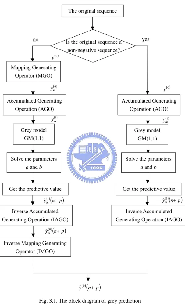
(26) p. bias = min y (0 ) (k). (3.9). k =1. and adding the bias term to the original data sequence. In this way, the original data sequence could be mapped into a new data sequence, which is expressed as ym (k) = y (0 ) (k) + bias (0 ). (3.10). and then the first predictive value could be obtained as. (. ). b ˆy m (0) ( p + 1) = 1 − e a ⋅ ⎛⎜ ym (0 ) (1 ) - ⎞⎟ e −ap a⎠ ⎝. (3.11). After taking away the bias, the first predictive value of the original sequence y (0 ) (k) is then found as ˆy (0) ( p + 1) = ˆy m (0) ( p + 1) - bias. (3.12). which will be employed to predict the matched disturbance. It is noted that (3.10) is usually called the mapping generating operation (MGO) and (3.12) is called the inverse mapping generating operation (IMGO). The block diagram of grey prediction is shown in Figure 3.1, and then a simple example of the application of grey prediction will be shown.. 18.

(27) The original sequence. no y (0 ). yes. Is the original sequence a non-negative sequence?. Mapping Generating Operator (MGO) y m(0 ). y (0 ). Accumulated Generating Operation (AGO). Accumulated Generating Operation (AGO). y m(1). y m(1). Grey model GM(1,1). Grey model GM(1,1). Solve the parameters a and b. Solve the parameters a and b. Get the predictive value. Get the predictive value ˆy m(1) (n+ p ). ˆy m(1) (n+ p ). Inverse Accumulated Generating Operation (IAGO). Inverse Accumulated Generating Operation (IAGO). ˆy m(0 ) (n + p ). Inverse Mapping Generating Operator (IMGO). ˆy (0 ) (n+ p ) Fig. 3.1. The block diagram of grey prediction. 19.

(28) Example of grey prediction for a given function x = cos(2π t ) , set the sampling time Ts = 0.01 sec and the displayed time interval is 0 ~ 2 sec. Here the minimum value of p is chosen, i.e., p = 4 . For the first grey prediction loop, the first four values of x, x(1) ~ x(4 ) , is chosen as the first data group and used to calculate y (1) ~ y (4 ) and z (1) ~ z (4 ) by AGO and IAGO, respectively. The matrices y and F in the matrix form of GM(1,1) can be obtained as ⎡0.99803⎤ ⎡ − 1.499 1⎤ ⎢ ⎥ y = ⎢ 0.99211⎥ , F = ⎢⎢ − 2.4941 1⎥⎥ ⎢⎣0.98229⎥⎦ ⎢⎣− 3.4813 1⎥⎦. and then the parameters a and b can be solved as ⎡0.0079375⎤ ⎡a ⎤ T -1 T ⎢b ⎥ = ( F F ) F y = ⎢ 1.0106 ⎥ ⎦ ⎣ ⎣ ⎦ Finally, the first predicted value is calculated as ˆy (0) (5) = 0.97518 which represents the 5th value of the original data sequence. As for the second grey prediction loop, the first data group would be shifted one position and appended the next component of the original data sequence, i.e., the new data group is x(2 ) ~ x(5) . Similarly, the next predicted value could be obtained by following the procedures operated in the first prediction loop. The remaining prediction loops would be finished in the same way, and the results are shown in Figure 3.2.. 20.

(29) (a). (b). Fig. 3.2 Results of the grey prediction. It should be noticed that in Fig. 3.1(a), the symbol ‘x’ represents the original data sequence, the symbol ‘y’ represents the predictive value, and the first four data are not shown since they would not be predicted. Fig. 3.1(b) is the predictive error.. 21.

(30) For the resulted sequence ˆy (0) (k ) , let’s check the following ratio between two consecutive data ˆy (0) (k + 1) = e − a , for k ≥ 2 (0) ˆy (k ). (3.13). Clearly, the ratios for k ≥ 2 are all the same and equal to e − a which shows that the sequence ˆy (0) (k ) decreases or increases monotonously with an exponential rate a. In other words, the GM(1,1) model is mainly suitable for monotone sequences approximately possessing a single exponential rate. Unfortunately, most of the physical sequences are changeable and not of single exponential rate. This implies the GM(1,1) model may not well predict most of the physical sequences. To reduce the prediction errors, some investigators employ a higher order grey model and some others try to modify the original GM(1,1) model. Here, a novel modified pseudo second-order grey model, called pseudo-GM(2,1) or PGM(2,1), is proposed which is not only as simple as the GM(1,1) model but also allows the predictive data to possess two exponential rates similar to the GM(2,1) model. It has been known that the GM(1,1) model adopts the latest p data where p ≥ 4 , and then the first predictive data of the i-th subsequence yi. (0). (. yi. (0). given as. ). = y (0) (i ), y (0) (i + 1), K , y (0) ( p + i − 1) , can be achieved from (3.8) and. expressed as ⎛ b ˆy i (0) ( p + 1) = 1 − e ai ⋅ ⎜⎜ yi (0 ) (1 ) - i ai ⎝. (. ). 22. ⎞ −ai p ⎟⎟ e ⎠. (3.14).

(31) where the development coefficient a i and grey input bi could be solved as mentioned before. Tracing back to the first predictive data of the (i-1)-th subsequence, we can get ⎛ b ⎞ ˆy i −1 (0) ( p + 1) = 1 − e ai −1 ⋅ ⎜⎜ yi −1 (0 ) (1 ) - i −1 ⎟⎟ e −ai −1 p a i −1 ⎠ ⎝. (. ). (3.15). In case that ai and ai-1 are not quite distinct, (3.14) and (3.15) will have good results for predicting y i. (0). (0). and y i −1 . However, when the difference between ai and ai-1. increased to a certain level, then it reveals that y i. (0). and y i −1. (0). are at least related to. two exponential rates. Intuitively, the GM(2,1) model should be a better choice for such situation, but it is much more complicated than the GM(1,1) model. In order to keep the simplicity of the GM(1,1) model, a modification is proposed as follows: ⎛ b e − (ai − ai −1 ) ⎞ −ai p ⎟e ˆy i (0) ( p + 1) = 1 − e ai ⋅ ⎜ yi (0 ) (1 ) - i ⎜ ⎟ a i ⎝ ⎠. (. ). (3.16). which changes bi into bi e − (ai − ai −1 ) . The performance of the PGM(2,1) model is expected to be better than that of the GM(1,1) model, and the comparisons will be shown later.. 23.

(32) Chapter 4 Controller Design The sliding-mode controller design will be presented in Chapter 4. However, before get into the sliding-mode controller design, the sliding-mode control (SMC) should be introduced. Thus, Section 4.1 is the introduction of the sliding-mode control, and then the novel sliding-mode controller design will be shown in Section 4.2. Finally, Section 4.3 will introduce the sliding-mode controller design incorporated with grey prediction.. 4.1 Introduction of Sliding-Mode Control Sliding mode is a particular system behavior of the variable structure system (VSS). Generally speaking, the rough definition of the variable structure system is that a system containing two or more subsystems and possessing some switching conditions which would be used to determine which subsystem should be presented under some specific situation. According to the tracing of the bibliography, the technology of the variable structure system had been applied to the motor control, and the sliding mode had been noticed in about the 1950s. But until the 1970s and the. 24.

(33) 1980s, the variable structure control (VSC) was studied and researched more and more widely, and more and more scholars threw themselves into this field. Variable structure control is a technology that makes the controlled system produce two or more subsystems, and then uses some purposely adding switching conditions to get the control goal. As for the sliding-mode control, a sliding surface S must be designed first and then the system trajectory would be forced to get into the sliding surface in a finite time, which is the so-called approaching condition or reaching condition, by using the designed control input. Besides, the system trajectory would stay within the hyperspace thereafter and move toward the control destination smoothly, which is the so-called sliding condition. It should be noticed that the equivalent control input would occur at the moment of S = 0 and the number of degree-of-freedom in the hyperspace is one less than that in the original system. The modern control technology contains both the variable structure control and the sliding-mode control, and the occurrence of the sliding mode is the main key point to distinguish between them [11]. As SMC is mentioned, it is undoubtedly that the robustness property for the system’s parametric uncertainty and external disturbances would be emphasized. For the matched disturbance, it can be completely eliminated if an infinite switching frequency exists. However, it’s a pity that the switching operations could not be. 25.

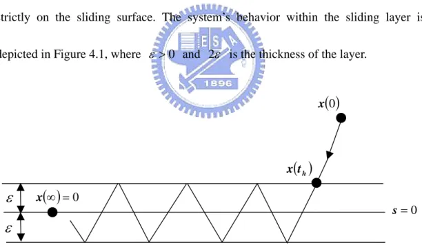
(34) finished immediately, no matter in the practical experiments or in the computer simulations. In other words, the switching operation would suffer from the hysteresis and the system trajectory would vibrate to and fro between both sides of the sliding surface at a very high frequency. Certainly, the switching term of the control input would also change at a very high frequency, and such unpredictable high-frequency oscillation phenomenon is the so called chattering. There are several methods to improve the chattering phenomenon and the most general one is the adoption of the sliding layer, which allows the system to stay just in the sliding layer instead of strictly on the sliding surface. The system’s behavior within the sliding layer is depicted in Figure 4.1, where ε > 0 and 2ε is the thickness of the layer. x (0 ). x (t h ). ε. x (∞ ) = 0. s=0. ε Fig. 4.1. The system’s behavior within the sliding layer. 26.

(35) 4.2 Conventional Sliding-Mode Controller Design In general, a linear time-invariant system suffering from matched disturbance can be described as x& = Ax + Bu + Bd ( x ,t ). (4.1.1). where x ∈ R n is the system state, u ∈ R m is the control input, A and B are constant matrices of appropriate dimensions, and d ( x ,t ) ∈ R m is the matched disturbance which would represent the parametric uncertainties and external disturbances. The sliding-mode control can theoretically suppress the matched disturbance with the hypothesis that the upper bound of the matched disturbance, denoted as d ( x ,t ) max for d ( x ,t ) or d i ( x ,t ) max , i = 1,2,L m , for i-th component of d ( x ,t ) , are known. The first step of the sliding-mode controller design is to choose an appropriate sliding vector. Let the sliding vector be. s = (CB ) Cx −1. where s = [s1. (4.1.2). s2 L sm ]. det (CB ) ≠ 0 , i.e., (CB ). T. −1. and the coefficient matrix C ∈ R m×n must satisfy that. exists. Taking the first derivative of (4.1.2) yields. −1 −1 s& = (CB ) Cx& = (CB ) CAx + u + d ( x ,t ). Based on the concept of equivalent control, i.e., s&. u = ueq. (4.1.3). = 0 , we have. ueq = −(CB ) CAx − d ( x ,t ) −1. (4.1.4). Then, with u = ueq , the system (4.1.1) in the sliding mode performs as. 27.

(36) (. ). −1 x& = I − B (CB ) C Ax. (4.1.5). which is nothing to do with the matched disturbance. In other words, the matched disturbance is completely eliminated while the system trajectory is restricted in the sliding mode. It has been known that no matter what C is,. (I − B(CB ) C )A −1. possesses m zero eigenvalues; besides, C should be designed to locate the other n-m. (. ). eigenvalues of I − B( CB ) −1 C A to guarantee the system stability, i.e., all the other. n-m eigenvalues must be located on the left half plan in s-domain or within the unit circle in z-domain. To develop the sliding-mode control algorithm, (4.1.3) is first transformed into the numerical form as. [. ]. −1 s&i = (CB ) CA i x + u i + d i ( x ,t ),. where. [(CB ). −1. i = 1,2,L m. ]. (4.1.6). CA i represents the i-th row vector of (CB ) CA . In order to suppress −1. the effect caused by d i ( x ,t ) , the control law is established as. [. ]. u i = − (CB ) CA i x − (γ i + σ i ) sign(s i ) −1. (4.1.7). where σ i > 0 and γ i = d i ( x ,t ) max . By using the control law (4.1.7), it is easy to find that s i s&i = −(γ i + σ i ) s i + s i d i ( x ,t ) ⎛ s d ( x ,t ) ⎞ ⎟ = −σ i s i − γ i s i ⎜⎜1 − i i ⎟ s γ i i ⎝ ⎠ < −σ i s i. (4.1.8). which guarantees the reaching and sliding condition. That means the system trajectory 28.

(37) will be driven to the sliding mode in a finite time and then approach the destination along the sliding surface. However, the use of sign(si) always generates undesirable high-frequency chattering phenomenon. To avoid such unwanted high-frequency response, sign(si) is often modified as ⎧ sign(s i ) , if s i > ε i ⎪ si sat (s i ,ε i ) = ⎨ , if s i ≤ ε i ⎪ εi ⎩. (4.1.9). where s i ≤ ε i is the so-called sliding layer with thickness 2ε i . Consequently, the control law (4.1.7) could be rewritten into. [. ]. u i = − (CB ) CA i x − (γ i + σ i ) sat (s i ,ε i ) −1. [ [. ] ]. ⎧− (CB )−1 CA i x − (γ i + σ i ) sign(s i ) , if s i > ε i ⎪ =⎨ si −1 , if s i ≤ ε i ⎪ − (CB ) CA i x − (γ i + σ i ) ε i ⎩. (4.1.10). which steers the system trajectory to the sliding layer within a finite time and makes the system trajectory moving smoothly without any chattering within there.. 4.3 Sliding-Mode Controller Design Combined with Grey Prediction Since it is known to all that the upper bound of the disturbances is very difficult to be calculated, the grey prediction method is used to predict the value of the matched disturbances. When the grey prediction applies into the sliding-mode controller design, the control law (4.1.7) could be rewritten as. 29.

(38) [. ]. −1 u i = − (CB ) CA i x − γ i ⋅ sign(s i ) − dˆ i (mT ),. for t ∈ [mT, (m+ 1)T ). (4.2.1). where T is the prediction period and dˆ i (mT ) is the predicted value of d i ( x ,t ) at t = mT . Intuitively, if d i ( x ,t ) can be well predicted by dˆ i ( x ,t ) , then the effects. caused by the matched disturbance could be effectively ameliorated. Besides, γ i is chosen to satisfy. γ i > d i ( x ,t ) − dˆ i (mT ). max. +σi. for t ∈ [mT, (m+ 1)T ), σ i > 0. (4.2.2). By using (4.2.1), it is easy to find that. [. ]. s i s&i = −γ i s i + s i d i ( x ,t ) − dˆ i (mT ) = −σ i s i − d i ( x ,t ) − dˆ i (mT ). max. [. ]. s i + s i d i ( x ,t ) − dˆ i (mT ). (4.2.3). < −σ i s i Clearly, the reaching and sliding condition s i s&i < −σ i si. is satisfied, which. guarantees the system trajectory reaching the sliding mode in a finite time and then approaching the destination along the sliding surface. In the same way, substituting the saturation function (4.1.9) into the control law (4.2.1) leads to. [. ]. −1 u i = − (CB ) CA i x − γ i ⋅ sat (s i ,ε i ) − dˆ i (mT ). [ [. for t ∈ [mT, (m+ 1)T ). ] ]. ⎧− (CB )−1 CA i x − γ i ⋅ sign(s i ) − dˆ i (mT ), if s i > ε i ⎪ =⎨ si ˆ −1 if s i ≤ ε i ⎪− (CB ) CA i x − γ i ⋅ − d i (mT ), εi ⎩ (4.2.4) which steers the system trajectory to the sliding layer in a finite time and makes it moving smoothly without any chattering.. 30.

(39) Next, let’s concentrate on the grey predicting scheme introduced in Chapter 3 by which the vector dˆ i ( x ,t ) could be determined. First, define the data sequence as y (0 ) (k ) = d i ( x ((m− p − 1 + k )T ),(m− p − 1 + k )T ) , k = 1,2 ,L , p , p ≥ 4 (4.2.5). which are required to predict d i ( x (mT ), mT ) at the moment t = mT , i.e., the value of y 0 ( p + 1) . However, the sequence in (4.2.5) is actually constructed by a series of disturbances, which could not be obtained via direct measurement. In other words, an indirect process should be adopted to achieve the sequence (4.2.5). Before getting into the indirect process, the sequence in (4.2.5) is re-expressed as d i ( x ((m− j )T ),(m− j )T ). for j = p , p − 1,L ,2 ,1. (4.2.6). for convenient. By applying the control algorithm (4.2.4) to (4.1.6), we have s&i = −γ i ⋅ sat (s i ,ε i ) + d i ( x ,t ) − dˆ i (mT ). for t ∈ [mT, (m+ 1)T ). (4.2.7). then the value of d i ( x ,t ) at t = mT could be derived as d i ( x (mT ), mT ) = s&i (mT ) + γ i ⋅ sat (s i (mT ),ε i ) + dˆ i (mT ). (4.2.8). which implies the data sequence (4.2.5) can be also calculated from d i ( x ((m− j )T ), (m− j )T ) = s&i ((m− j )T ) + γ i ⋅ sat (s i ((m− j )T ),ε i ) + dˆ i ((m− j )T ). (4.2.9). where j = p , p − 1,L ,2 ,1 . Unfortunately, the differential term s&i ((m− j )T ) is still not measurable; instead, it is approximated as s&i ((m− j )T ) ≈. s i ((m− j + 1)T ) − s i ((m− j )T ) T. (4.2.10). for j = p, p − 1,L ,2 , which is not suitable for the case of j = 1 due to the fact that 31.

(40) s i (mT ) is not attainable at t = mT . In other words, it is impossible to adopt dˆ i (mT ). which should be calculated from s i (mT ) in the control algorithm (4.2.4) at t = mT . In order to avoid such situation, the term s&i ((m− 1)T ) is approximated as s i ((m− 0 .5)T ) − s i ((m− 1)T ) . However, there is an assumption here that the first 0. 5 T. predictive value of the data sequence (4.2.9), dˆ i (mT ) , can be obtained within the time interval of t ∈ ((m− 0.5)T, mT ) . Hence, the data sequence (4.2.9) can be obtained approximately as d i ( x ((m− j )T ),(m− j )T ) ≈. ⎧ s i ((m− j + 0 .5)T ) − si ((m− j )T ) + γ i ⋅ sat (si ((m− j )T ),ε i ) + dˆ i ((m− j )T ) ⎪ 0.5 T ⎪ for j = 1 ⎪ ⎨ ⎪ si ((m− j + 1)T ) − si ((m− j )T ) + γ ⋅ sat (s ((m− j )T ),ε ) + dˆ ((m− j )T ) i i i i ⎪ T ⎪ for j = 2,3,L , p ⎩. which is used for the grey prediction of dˆ i (mT ) .. 32. (4.2.11).

(41) Chapter 5 Simulation Results. The general dynamic equation of a DC motor mounted with a payload derived in Chapter 2 is depicted again as (5.1) x& = Ax + Bu + Bd1. where A = −. (5.1). Kt Kb Kt , B= , x means the rotational velocity, u is Ra ( J m + J ) Ra ( J m + J ). the input voltage, and d 1 represents some uncertainties and the external disturbances. However, for the consideration of robustness of the designed controller, the mounted payload could be any shape or material; i.e., the rotational inertia of payload, J , is thought as unknown. If this unknown parameter is also categorized as disturbance, defined as d 2 , (5.1) can be simplified as ~ x& = A1 x + B1u + B1 d. where A1 = −. (5.2). Kt Kb Kt ~ , B1 = , and d = d1 + d 2 , which includes the parametric Ra J m Ra J m. uncertainties and the external disturbances. Since speed control is the control goal, it would be more convenient that changing the state variable from speed of DC motor to the error of speed. Thus, (5.2) can be further rewritten as ~ e& = A1e+ B1u + B1 d + A1 ω d. (5.3). where e = ω − ω d is error of speed, and ω d is the desired speed.. 33.

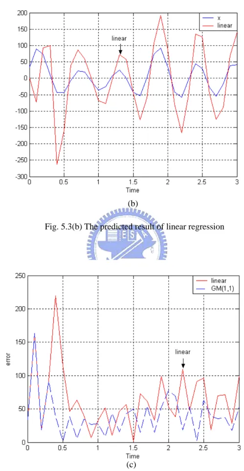
(42) The numerical simulations of the performance of grey predictor for distinct forms of the disturbances, the comparisons with the linear regression method, and the comparison between the traditional sliding-mode control and the novel sliding-mode control incorporated with grey predictor will be shown in this chapter. The given disturbances are designed as the combination of sinusoidal waveforms. The types of sinusoidal disturbances would vary from low frequency to high frequency, and from simple combinations to more and more complicated forms. Because grey prediction needs at least four data to work, grey predictor would not predict the first four data. The first part of the simulation results is the comparison between the grey predictor and the linear regression method. The second part is the comparison between the GM(1,1) model and the modified PGM(2,1) model, and the last part is the comparison between the traditional sliding-mode control and the sliding-mode control combined with grey predictor. In the following simulation result figures, the symbol ‘x’ presents the given disturbance signal, ‘linear’ means the linear regression method.. 34.

(43) Comparison I : The comparisons between the GM(1,1) model and the linear regression method will be shown as follows:. ◆ Case 1 : d = 11 cos(7 t ) + 55 sin(9 t ) + 15 cos(5.3 t ) cos(6.7 t ). (a) Fig. 5.1(a) The predicted result of GM(1,1). 35.

(44) (b) Fig. 5.1(b) The predicted result of linear regression. (c) Fig. 5.1(c) The predictive error of GM(1,1) and linear regression 36.

(45) ◆ Case 2 : d = 11 cos(7 t ) + 55 sin(9 t ) + 15 cos(5.3 t ) cos(6.7 t ) + 22 sin(4.5 t ) cos(3.3 t ). (a) Fig. 5.2(a) The predicted result of GM(1,1). (b) Fig. 5.2(b) The predicted result of linear regression. 37.

(46) (c) Fig. 5.2(c) The predictive error of GM(1,1) and linear regression. ◆ Case 3 :. d = 11cos(7 t ) + 5 sin(9 t ) + 54 sin(11t ) + 23 cos(4.4 t ) cos(8.6 t ) + 33 sin(2.1t ) cos(5.2 t ) + 29 sin(3.5 t ). (a) Fig. 5.3(a) The predicted result of GM(1,1) 38.


(48) ◆ Case 4 : d = 11 cos(7πt) + 29 sin(9πt). (a) Fig. 5.4(a) The predicted result of GM(1,1). (b) Fig. 5.4(b) The predicted result of linear regression. 40.

(49) (c) Fig. 5.4(c) The predictive error of GM(1,1) and linear regression. ◆ Case 5 : d = 11 cos(7π t ) + 29 sin(9π t ) + 17 cos(3.7π t ) sin(5.4π t ). (a) Fig. 5.5(a) The predicted result of GM(1,1) 41.


(51) Comparison II: The comparisons between the GM(1,1) model and the modified PGM(2,1) model will be shown as follows:. ◆ Case 1 : d = 11 cos(7 t ) + 55 sin(9 t ) + 15 cos(5.3 t ) cos(6.7 t ). (a) Fig. 5.6(a) The predicted results of GM(1,1) and PGM(2,1). 43.

(52) (b) Fig. 5.6(b) The predictive error of GM(1,1) and PGM(2,1). ◆ Case 2 : d = 11 cos(7 t ) + 55 sin(9 t ) + 15 cos(5.3 t ) cos(6.7 t ) + 22 sin(4.5 t ) cos(3.3 t ). (a) Fig. 5.7(a) The predicted results of GM(1,1) and PGM(2,1) 44.

(53) (b) Fig. 5.7(b) The predictive error of GM(1,1) and PGM(2,1). ◆ Case 3 :. d = 11cos(7 t ) + 5 sin(9 t ) + 54 sin(11t ) + 23 cos(4.4 t ) cos(8.6 t ) + 33 sin(2.1t ) cos(5.2 t ) + 29 sin(3.5 t ). (a) Fig. 5.8(a) The predicted results of GM(1,1) and PGM(2,1) 45.

(54) (b) Fig. 5.8(b) The predictive error of GM(1,1) and PGM(2,1). ◆ Case 4 : d = 11 cos(7πt) + 29 sin(9πt). (a) Fig. 5.9(a) The predicted results of GM(1,1) and PGM(2,1) 46.

(55) (b) Fig. 5.9(b) The predictive error of GM(1,1) and PGM(2,1). ◆ Case 5 : d = 11 cos(7π t ) + 29 sin(9π t ) + 17 cos(3.7π t ) sin(5.4π t ). (a) Fig. 5.10(a) The predicted results of GM(1,1) and PGM(2,1). 47.

(56) (b) Fig. 5.10(b) The predictive error of GM(1,1) and PGM(2,1). 48.

(57) Comparison III: The comparisons between the traditional sliding-mode control and the novel sliding-mode control incorporated with grey predictor will be shown as follows:. ◆ Case 1 : d = 11 cos(7 t ) + 55 sin(9 t ) + 15 cos(5.3 t ) cos(6.7 t ). (a) Fig. 5.11(a) The simulation result of the novel sliding mode control. 49.

(58) (b) Fig. 5.11(b) The simulation result of traditional sliding mode control. ◆ Case 2 : d = 11 cos(7 t ) + 55 sin(9 t ) + 15 cos(5.3 t ) cos(6.7 t ) + 22 sin(4.5 t ) cos(3.3 t ). (a) Fig. 5.12(a) The simulation result of the novel sliding mode control. 50.

(59) (b) Fig. 5.12(b) The simulation result of traditional sliding mode control. ◆ Case 3 :. d = 11cos(7 t ) + 5 sin(9 t ) + 54 sin(11t ) + 23 cos(4.4 t ) cos(8.6 t ) + 33 sin(2.1t ) cos(5.2 t ) + 29 sin(3.5 t ). (a) Fig. 5.13(a) The simulation result of the novel sliding mode control. 51.

(60) (b) Fig. 5.13(b) The simulation result of traditional sliding mode control. ◆ Case 4 : d = 11 cos(7πt) + 29 sin(9πt). (a) Fig. 5.14(a) The simulation result of the novel sliding mode control 52.

(61) (b) Fig. 5.14(b) The simulation result of traditional sliding mode control. ◆ Case 5 : d = 11 cos(7π t ) + 29 sin(9π t ) + 17 cos(3.7π t ) sin(5.4π t ). (a) Fig. 5.15(a) The simulation result of the novel sliding mode control. 53.

(62) (b) Fig. 5.15(b) The simulation result of traditional sliding mode control. 54.

(63) Chapter 6 Conclusions. This thesis has proposed a new method adopting grey theory for the prediction of the disturbances. The substance of the grey theory is utilizing the lacking data on hand to pick up the significant information and then go further and further until reaching the destination. Grey predictor has a well performance of the disturbances prediction by using only four data and simple calculations instead of a large amount of data and the complicated computations. It should be known that grey predictor is a low-frequency predictor so it is not suitable for the disturbances with rapid variations, such as white noise. The simulation results of the PGM(2,1) model and the sliding-mode control combined with grey predictor applied to speed control of DC motor are also presented. These results demonstrate that the PGM(2,1) model has better performance than the GM(1,1) model and the grey predictor indeed solves the problem of estimating the upper bound of the disturbances. However, the results of the PGM(2,1) model still has the problem of phase delay, some advanced modifications could be applied to the original GM(1,1) model to make it more efficient for the prediction of the disturbances.. 55.

(64) References [01] C.D. Johnson, "Theory of Disturbance Accommodating Controllers," Control and Dynamic Systems: Advances in Theory and Applications, vol. 12, New York,. Academic Press, 1976. [02] K.K. Chew and M. Tomizuka, "Digital Control of Repetitive Errors in Disk-Drive Systems," IEEE Control Systems Magazine, vol. 10, No. 1, pp. 16-20, January 1990. [03] T. Umeno, T. Kaneko, and Y. Hori, “Robust servosystem design with two degrees of freedom and its application to novel motion control of robot manipulators,” IEEE Trans. Ind. Electron., vol. 40, pp. 473–486, Oct. 1993. [04] Xia Jun, "A grey system approach applied to catchment hydrology," Uncertainty Modeling and Analysis, Proceedings, First International Symposium on ,. pp.7-12, Dec. 1990. [05] R. Hult, "Grey-level morphology combined with an artificial neural networks approach for multimodal segmentation of the Hippocampus," Image Analysis and Processing, 2003.Proceedings. 12th International Conference on , pp. 277 -. 282, 17-19 Sept. 2003 [06] Rong-Jong Wai; Rou-Yong Duan; Li-Jung Chang, "Grey feedback linearization speed control for induction servo motor drive," Industrial Electronics Society,. 56.

(65) 2001. IECON '01. The 27th Annual Conference of the IEEE , 29 Nov.-2,pp. 580. - 585 vol.1, Dec. 2001 [07] M. Dong; Z. Yan; Y. Taniguchi, “Fault diagnosis of power transformer based on model-diagnosis with grey relation,” Properties and Applications of Dielectric Materials, 2003. Proceedings of the 7th International Conference on , pp.1158 -. 1161 vol.3, 1-5 June 2003 [08] Chang-Yung Kung; Chung Chao; Ta-Lin Chien, “An application of GM (1,1) model for automobile industry,” Systems, Man and Cybernetics, 2003. IEEE International Conference on , pp. 3244 - 3250 vol.4, 5-8 Oct. 2003. [09] Shiuh-Jer Huang; Chien-Lo Huang, “Control of an inverted pendulum using grey prediction model,” Industry Applications, IEEE Transactions on , Volume: 36 , Issue: 2 , pp. 452 – 458, March-April 2000 [10] Keh-Tsong Li and Yon-Ping Chen, “Sliding-Mode Controller Design with Grey Prediction for Matched Disturbance,” International Journal of Fuzzy System, Vol. 6, No. 1, pp.1-8, March 2004 [11] 可變結構控制設計，陳永平，張浚林編著，全華科技圖書股份有限公司。 [12] 灰色系統理論與應用，鄧聚龍著，高立圖書有限公司。 [13] 灰色系統基本方法及其應用，翁慶昌，陳嘉欉，賴宏仁編著，高立圖書有限公司。. 57.

(66)