以圖型自同構為基礎之自動接線驗證樣本產生器

全文

(1)國立交通大學電子工程學系碩. 電子研究所碩士班士. 論. 文. 以圖型自同構為基礎之自動接線驗證樣本產生器 On Automatic Pattern Generation for Interconnect Verification Based on Graph Automorphism. 研究生：周貞伶指導教授：周景揚博士. 中華民國九十三年六月.

(2) 以圖型自同構為基礎之自動接線驗證樣本產生器. On Automatic Pattern Generation for Interconnect Verification Based on Graph Automorphism. 研究生：周貞伶. Student: Chen-Ling Chou. 指導教授：周景揚博士. Advisor: Dr. Jing-Yang Jou. 國立交通大學電子工程學系電子研究所碩士班碩士論文 A Thesis Submitted to Institute of Electronics College of Electrical Engineering and Computer Science National Chiao Tung University In Partial Fulfillment of the Requirements For the Degree of MASTER OF SCIENCE In Electronics Engineering June 2004 Hsinchu, Taiwan, Republic of China. 中華民國. 九十三年. 六月.

(3) 以圖型自同構為基礎之自動接線驗證樣本產生器研究生：周貞伶. 指導教授：周景揚博士. 國立交通大學電子工程學系電子研究所碩士班. 摘. 要. 在大型系統晶片 (system-on-a-chip, SoC) 設計中，嵌入式核心(embedded cores) 的使用正大量的增加。高複雜度的系統晶片設計，使得設計驗證對系統整合者來說是個很大的挑戰。為了降低以嵌入式核心為基礎的設計驗證的複雜度，連接埠順序障礙模型 (port-order-fault，POF) 已經被提出，其對應的驗證向量產生器也已經發展好了。在本論文中，為了解決大型系統晶片連接驗證的問題，我們在連接埠順序障礙模型之下提出了一個以圖形自同構 (graph automorphism) 為基礎的演算法來改善這個自動驗證向量產生器的效率。此外，這個演算法也可以運用於計算電路的輸入對稱的最大集合。我們測試了一些 ISCAS-85 和有較多輸入連接埠的 MCNC 電路。由實驗結果顯示，這個演算法可以在更少的時間下產生更有效的驗證向量。. i.

(4) On Automatic Pattern Generation for Interconnect Verification Based on Graph Automorphism Student: Chen-Ling Chou Advisor: Dr. Jing-Yang Jou. Department of Electronics Engineering & Institute of Electronics National Chiao Tung University. Abstract Embedded cores are being increasingly used in the design of large system-on-a-chip (SoC). High complexities of SoC designs lead the design verification to be a challenge for system integrators. To reduce the verification complexity, the port-order-fault (POF) model has been proposed and the corresponding verification pattern generation has been developed for verifying core-based designs. This thesis proposes a graph automorphism-based algorithm to improve the efficiency of the automatic verification pattern generation (AVPG) for SoC interconnect verification based on the POF model. Furthermore, this algorithm can be applied to compute maximal sets of symmetric inputs of circuits. We conduct the experiments on ISCAS-85 and some MCNC benchmarks with large inputs of circuits. The experimental results demonstrate that our approach generates more efficient patterns with less CPU time.. ii.

(5) ACKNOWLEDGEMENTS I would like to express my sincere gratitude to my advisor, Professor Jing-Yang Jou (周景揚), for his insightful suggestion and patient guidance throughout the course of this work in the two years of my graduate life. I am still very grateful for his help in many other matters, academically and socially. I am also indebted to Chun-Yao Wang ( 王俊堯 ) and Geeng-Wei Lee ( 李耿維 ), for their great help and constructive suggestions on my research. Thanks also go to all members in the Electronic Design Automation Lab for their friendship and all members of the intramural badminton team. Finally I have to show my deepest gratefulness to my parents, 周乾德 and 蔣慧月, my sister, 周芳俞, and my boyfriend, Hung-Chih Lai (賴鴻志). Without their support and love, this work would not be complete.. iii.

(6) Contents Chinese Abstract .......................................................................................................................i English Abstract.......................................................................................................................ii Acknowledgements................................................................................................................ iii Contents ..................................................................................................................................iv List of Tables ...........................................................................................................................v List of Figures.........................................................................................................................vi Chapter 1. INTRODUCTION................................................................................................1. Chapter 2. PRELIMINARY...................................................................................................6. 2.1. POE MODEL......................................................................................................6 2.2. UNDETECTED PORT SEQUENCES (UPSS) REPRESENTATION ..............................8 2.3. PREVIOUS WORK ...............................................................................................9 Chapter 3. GRAPH AUTOMORPHISM-BASED AVPG ...................................................12. 3.1. PATTERN GENERATION ....................................................................................13 3.2. GRAPH AUTOMORPHISM ALGORITHM .............................................................18 3.3. UPSS CALCULATION WITH AUTOMORPHISM TECHNIQUE ................................25 Chapter 4. EXPERIMENTAL RESULTS ...........................................................................32. Chapter 5. APPLICATIONS ...............................................................................................35. 5.1. ABOUT SYMMETRIC.........................................................................................35 5.2. SYMMETRIC WITH GA ALGORITHM .................................................................38 5.3. EXPERIMENTAL RESULTS ................................................................................41 Chapter 6. CONCLUSIONS................................................................................................45. REFERENCES ....................................................................................................................R-1 VITA....................................................................................................................................V-1. iv.

(7) List of Tables Table 3.1. All possible pattern sets .......................................................................................... 16 Table 3.2. θ 25 pattern sets ....................................................................................................... 18 Table 4.1. Comparisons on experimental results of SAA approach and GA approach............ 34 Table 5.1. Comparisons on experimental results of previous approach in [38] and GA approach .......................................................................................................................... 43 Table 5.2. Results of some MCNC benchmarks ...................................................................... 44. v.

(8) List of Figures Figure 1.1. The schemes of interconnection testing and interconnection verification ............... 4 Figure 2.1. The schematic representation of EFPS 1234 and EPS 1423.................................... 7 Figure 2.2. The flowchart of the POE-based AVPG................................................................ 10 Figure 2.3. Hierarchical relations among the different approaches.......................................... 11 Figure 3.1. Error activation...................................................................................................... 15 Figure 3.2. Possible further pattern sets in A5 and A6 ............................................................ 16 Figure 3.3. An example of graph G and its automorphisms .................................................... 19 Figure 3.4. An undirected graph G and its Adj(G) .................................................................. 20 Figure 3.5. Disjoint graph, complete graph and cycle graph ................................................... 24 Figure 3.6. UPSs_Calculation with GA technique................................................................... 26 Figure 3.7. Graph Automorphism (GA) technique .................................................................. 28 Figure 3.8. Verification pattern set with automorphism message (AM) .................................. 29 Figure 3.9. Complete AVPG flow ........................................................................................... 30 Figure 3.10. Pseudo code of AVPG with GA technique.......................................................... 31 Figure 5.1. Complete ACSP flow ............................................................................................ 40 Figure 5.2. Pseudo code of ACSP with GA technique ............................................................ 41. vi.

(9) Chapter 1 Introduction Spurred by process technology leading to the availability of more than 1 million gates per chip, and more stringent requirements upon time-to-market and performance constraints, system level integration and platform-based design [3] are evolving as a new paradigm in system designs. A multitude of components that are needed to implement the required functionality make it hard for a company to design and manufacture an entire system in time and within reasonable cost. Hence, design reuse and reusable building blocks (cores) trading are becoming popular in the system-on-a-chip (SoC) era. However, present design methodologies are not enough to deal with cores which come from different design groups and are mixed and matched to 1.

(10) create a new system design. In particular, verifying whether a design satisfies all requirements is one of the most difficult tasks. Usage of cores divides the IC design community into two groups: core providers and system integrators. In traditional system-on-board (SoB) design, the components that go from provider to system integrator are ICs, which are designed, verified, manufactured, and tested. The system integrator verifies the design by using these components as fault-free building blocks. SoB verification is limited to detecting faults in the interconnection among the components. Similarly, in SoC design, the components are cores. The system integrator verifies the design by using the cores as design error-free building blocks. The focus of this core-based design verification should be on how the cores communicate with each other [13]. However, before the interface verification, the interconnection between the cores in an SoC have to be verified first. This is because the SoC integrator has to connect a large number of ports (hundreds or even thousands of ports) in an SoC. The likelihood of interconnection misplacements between the cores is high. Furthermore, the correct interconnection between the cores is the minimum requirement to verify the interface protocols. In other words, if the interconnections between the cores are misplaced, the process of the verification on the interface between the cores will be in vain. Thus, the interconnection verification can be conducted as the first step to the interface verification between the cores in an SoC. Most previous work in testing interconnection focused on the development of deterministic tests for interconnection between chips at the board level [7, 8]. The main purpose is to test if the interconnections are connected properly (neither short nor open). In the interconnection testing phase, the basic assumption for a system under test is that 2.

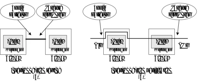
(11) the system design is correct, and the faults are due to manufacturing defects on interconnection among components. For the core-based SoC design verification, however, the system is not fully verified yet and the most of system design errors are due to the incorrect interconnection among predesigned cores. The incorrect interconnections are normally introduced by the misinterpretation of port description of IP cores, and this misinterpretation is usually caused by some factors, such as ambiguous or cryptic port names, Big Endian or Little Endian byte order of address bus, etc. Therefore, the extension of these board level testing methods is inadequate for connectivity-based design verification. Fig. 1.1 (a) and (b) shows the schemes to demonstrate the processes of interconnection testing and interconnection verification, respectively. In the interconnection testing, the engineers focus on the success of implementation of interconnected wires between block1 and block2. The testing patterns and corresponding responses are applied and observed at the ends of the interconnects to check whether the interconnects are manufactured correctly. On the other hand, in the interconnection verification, the system integrators verify whether the interconnections between block1 and block2 are located in the correct ports. They apply the verification patterns to primary inputs (PIs) of the integrated design, then observe the corresponding responses in primary outputs (POs) of the integrated design, and match them against the specification instead.. 3.

(12) apply patterns. observe responses. core1. core2. wrapper. wrapper. block1. block2. observe responses. apply patterns. PIs. interconnection testing (a). core1. core2. wrapper. wrapper. block1. block2. POs. interconnection verification (b). Figure 1.1. The schemes of interconnection testing and interconnection verification. By creating the testbenches at a high level, a connectivity-based design fault model, port-order-fault (POF), proposed in [17], is used for reducing the time on core-based design verification [18]. And the superset of all automorphism (SAA) technique is proposed in [19] to accelerate the AVPG and reduce the size of verification pattern set. In this thesis, we propose a graph automorphism-based algorithm to further reduce the size of verification pattern set. This algorithm also can compute maximal sets of symmetric inputs of circuits, which are important to design verification and diagnosis [9, 10, 12, 16], as well as technology mapping [5, 11, 14]. In general, the manufacturing defects are called faults. Since this approach is conducted for design verification rather than chip testing, we rename the POF model as port-order-error (POE) without changing the model definition. We exploit the IEEE P1500 wrappers and user defined Test Access Mechanisms (TAMs) to propagate the verification patterns from PIs to the wrappers in the predecessor of the core under verification (CUV) and to propagate responses of the CUV to POs. The integration verification mechanism with the IEEE P1500 4.

(13) standard-under-development is the same with that introduced in [18]. The remainder of this thesis is organized as follows: the POE model and previous work are introduced in Chapter 2. Chapter 3 describes the graph automorphism (GA) technique in the AVPG. The experimental results are shown in Chapter 4 and the applications of symmetric detection are shown in Chapter 5. Chapter 6 concludes the thesis.. 5.

(14) Chapter 2 Preliminary 2.1. POE Model The POE model belongs to the group of pin-errors models [1], which assumes that an erroneous cell has at least two I/O ports misplaced. It also assumes that the components are error free and only the interconnections among the components could be erroneous. There are three types of POEs [17]. Definition 2.1: The type I POE is at least an output misplaced with an input. The type II POE is at least two inputs misplaced. The type III POE is at least two outputs misplaced. It has been proven that the type II POEs dominate the other two types of 6.

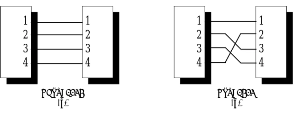
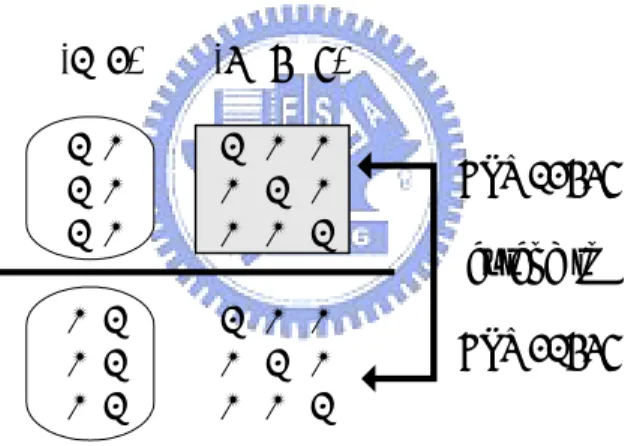
(15) POEs [18]. Hence, in this thesis, the AVPG focuses on the type II POEs solely. Definition 2.2: A port sequence is an input port number permutation that indicates the relative positions among these input ports. Definition 2.3: The error-free-port-sequence (EFPS) is a port sequence that none of the input ports were misplaced. For an N-input core, its input variables are numbered from 1 to N. The number of the input variable permutations is N! and these N! permutations. represent. the. N!. port. sequences. of. the. core.. Except. the. error-free-port-sequence, the remaining (N!-1) port sequences represent those corresponding cores with particular POEs and are called erroneous-port-sequences (EPSs). In this thesis, the POEs and the EPSs are used exchangeably. Given a 4-input core, the input ports are numbered from 1 to 4. Any input port numbers permutation is a port sequence of the core. It has 4! port sequences totally. The only one EFPS is 1234, the remaining (4!-1) port sequences are EPSs. The EPS 1423 represents the port 4 is connected to the location of port 2, the port 2 is connected to the location of port 3, and the port 3 is connected to the location of port 4. The schematic representation of EFPS 1234 and EPS 1423 are shown in Fig. 2.1 (a) and Fig. 2.1 (b), respectively.. 1 2 3 4. 1 2 3 4. 1 2 3 4. EFPS=1234 (a). 1 2 3 4 EPS=1423 (b). Figure 2.1. The schematic representation of EFPS 1234 and EPS 1423.. 7.

(16) 2.2. Undetected Port Sequences (UPSs) Representation Typically, the automatic pattern generator for functional errors, such as transition faults [6], or manufacturing faults, such as stuck-at-fault (SAF) [15], builds fault list explicitly first to explore how many faults have to be detected, and then generates random patterns and deterministic patterns to detect these faults in the fault list. For the POE-based AVPG, the error list is not enumerated explicitly. This is because the total number of POEs in an N-input core is (N!-1). This number grows rapidly when N increases, for instance, as N = 70, N!-1 ≈ 1.2×10100. Instead, an implicit representation is used to indicate the remaining undetected port sequences (UPSs). According to this implicit representation, we can realize exactly what the remaining UPSs are and the further verification patterns can be generated accordingly in the verification pattern generation. The following example demonstrates this implicit UPSs representation. Given an 8-input core, the input ports are numbered from 1 to 8. The UPSs representation (12345678) represents the UPSs that caused by all possible misplacements among the port numbers in the same group, i.e. port 1 to port 8. The number of undetected POEs is 8!-1, and the 1 in the 8! accounts for the error free port sequence. The UPSs representation (125)(4)(3678) indicates the UPSs that caused by all possible misplacements among the port numbers 1, 2 and 5 and/or all possible misplacements among the port numbers 3, 6, 7 and 8. The number of the undetected POEs is 3! × 1! × 4!-1. Please note that the port number 4 is the only one element in the second group. It means that the port sequences whose port number 4 in the wrong position are not represented by this UPSs representation. The order of the groups in the UPSs representation is irrelevant, neither is the order of the numbers in each UPSs 8.

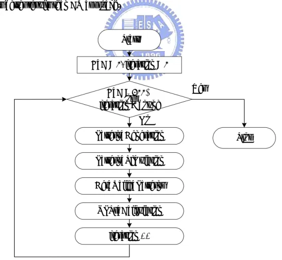
(17) group. For example, the UPSs (125)(4)(3678) can also be expressed as (4)(215)(8763). The UPSs (12)(3)(4)(5)(6)(78) contain 4 port sequences and they are 12345678, 21345678, 12345687 and 21345687. The UPS representation (1)(2)(3)(4)(5)(6)(7)(8) has eight groups and each group has only one element; therefore, no misplacement could be occurred in each group. The number of the undetected POEs is 1!×1!×1!×1!×1!×1!×1!×1!-1=0. Hence, (1)(2)(3)(4)(5)(6)(7)(8) represents 8!-1 POEs are all detected. If the UPSs representation is induced from (12345678) to (1)(2)(3)(4)(5)(6)(7)(8), all POEs are detected.. 2.3. Previous Work The AVPG for verifying the interconnect in a core-based design is proposed in [18]. Its flowchart is shown in Fig. 2.2 again. The AVPG reads the combinational core and generates heuristic patterns. The patterns simulation results determine the valid verification patterns. Then the UPSs are calculated in UPSs_Calculation stage, so that more further verification patterns can be generated accordingly. When the error coverage (E_C) reaches 100%, i.e., the verification patterns for detecting all EPSs are generated, or the iterations are over the bound, the AVPG will be terminated. The UPS’s calculation (UPSs_Calculation) procedure shown in Fig. 2.2 determines what the remaining UPSs are and guides the further pattern generation. If the results of UPS’s calculation are not precise enough, some of the further verification patterns could be redundant and the processing time to reach the desired error coverage will increase. In [18], the characteristic vector (CV) approach of determining the remaining UPSs encountered this weakness. However, the superset of all automorphisms (SAA) 9.

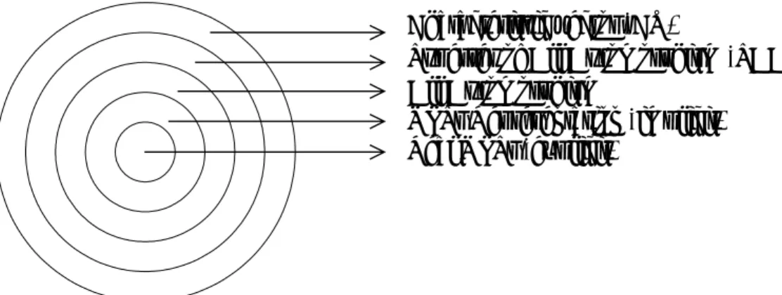
(18) technique proposed in [19] improves the weakness mentioned and indeed increases the AVPG efficiency. This fact can be seen in Fig. 2.3. Fig. 2.3 is a drawing from [19], which shows the hierarchical relations on computing remaining UPSs between the CV approach [18] and the SAA approach [19]. It has five levels from the center to the boundary. The first level represents the set of real remaining UPSs explicitly. The second level is the implicit UPS representation of the first level. The third level represents the UPSs that are obtained by the automorphism approach. The SAA approach and CV approach are shown in the fourth and fifth levels, respectively. Since the UPSs in the inner levels are the subset of the outer levels, the SAA approach really gets better results than CV approach.. Start. E_C = 0, iteration = 0. E_C = 100% or iteration > bound. Yes. No. Pattern_Generation. Stop. Pattern_Simulation. Get_Valid_Patterns. UPSs_Calculation iteration ++. Figure 2.2. The flowchart of the POE-based AVPG. 10.

(19) Characteristic vector (CV) Superset of All Automorphism (SAA) All Automorphism UPSs Representation (implicit) Real UPSs (explicit). Figure 2.3. Hierarchical relations among the different approaches.. 11.

(20) Chapter 3 Graph Automorphism–based AVPG We observe that the stages which profoundly influence the efficiency of AVPG are Pattern_Generation and UPSs_Calculation. Thus, in addition to advancing the UPSs_Calculation stage like [19], this thesis proposes a new pattern generation procedure as well, which corresponds to the proposed UPSs_Calculation. In this chapter, we first explain the new Pattern_Generation procedure. Then we introduce the graph automorphism algorithm. The new UPSs_Calculation procedure based on the graph automorphism algorithm is described in the last section.. 12.

(21) 3.1. Pattern Generation Definition 3.1 : For an N-input combinational core, the exhaustive pattern set is defined as ΦN. The size of ΦN is the number of patterns in ΦN, and is denoted as |ΦN| and |ΦN| equals 2N. Definition 3.2 : The set that consists of all patterns with m 1s and (N-m) 0s is denoted as θ mN ,where m∈ [0, 1, 2, . . ., N -1, N]. The size of θ mN is the number of patterns in θ mN and is denoted as | θ mN | and | θ mN | equals CmN . Example 3.1:. For a 4-input core, Φ4 is the exhaustive pattern set with 4 bits. |Φ4|. = 24 = 16. θ 04 ={0000}, | θ 04 | = C04 =1. θ14 ={1000, 0100, 0010, 0001}, | θ14 | = C14 =4.. θ 24 = {1100, 1010, 1001, 0110, 0101, 0011}, | θ 24 | = C24 = 6. θ 34 = {1110, 1101, 1011, 0111}, | θ 34 | = C34 =4. θ44 = {1111}, | θ44 |= C44 =1. The target of AVPG is to generate valid verification patterns such that all N!-1 POEs are detected. To detect a POE, the error effect has to be activated first. If the error effect is not activated, it surely cannot be propagated out for detection. Thus, all N!-1 POEs have to be activated during the Pattern_Generation stage. For general cases, all remaining POEs have to be activated in each iteration. To activate a POE, the logic assignments of the corresponding input ports cannot be all the same. For example, to activate the EPS 1243, the assignments of port 3 and port 4 have to be different, either port 3 is assigned 0, port 4 is assigned 1, or vice versa. Furthermore, to increase the AVPG efficiency, the generated verification pattern cannot be repeated.. Lemma 3.1: Given a pattern T ∈ θmN , there are m 1s and (N-m) 0s in T. If the pattern 13.

(22) T turns to T’ after a EPS λ, then T’ ∈ θmN and is a permutation of T byλ.. Theorem 3.1: θmN can activate all (N!-1) POEs where m ∈[1, 2, …, N-2, N-1]. [18] Proof: θmN contains all patterns with m 1s and (N-m) 0s. According to Lemma 3.1, there must exist a pair of patterns T and T’ ∈ θmN that corresponds to the original pattern T and the activated pattern T’ for each POE. Thus, (N!-1) POEs are all activated by θmN for m ∈[1, 2, …, N-2, N-1].. Q.E.D.. k Theorem 3.2: For an N-input core, the pattern set ∈ θ m11 Х θ m22 Х … Х θ mk with. n. n. n. n1 + n2 + …+ nk =N, 0≦mp≦np where p = 1,2,…,k and there being at least one group with different logic assignments can activate all (n1!) × (n2!) × ··· × (nk!)-1 errors in the UPSs ( a1a2 L an1 )(b1b2 Lbn2 ) L ( r1r2 L rnk ) .. θ mn can activate (n1!-1) POEs where m1∈ [1,. Proof : According to Theorem 3.1,. 1. 1. θ mn Х θ mn is to repeat θ mn Cmn times and to repeat θ mn Cmn. 2,…, n1-1]. Obviously,. 1. 2. 1. 2. 2. 1. 1. 2. 1. 2. 2. 1. θ mn with a set of θ mn can activate (n1!)-1 POEs,. times. For each pattern in. 2. 1. 2. 1. θ mn Х θ mn22 can activate (n1!)×(n2!)-1 POEs. We can extend this to k groups, therefore, 1. 1. each pattern set ∈ θ m11 Х θ m22 Х…Х n. n. θ mn can activate (n1!)×(n2!)×···×(nk!)-1 errors, k. k. same as the number of POEs in the UPSs ( a1a2 L an1 )(b1b2 L bn2 ) L ( r1r2 L rnk ) . Q.E.D. The simulation results of the verification patterns are observed to determine which activated POEs are propagated to POs. The error effects are propagated to POs if there 14.

(23) exists different responses among these verification patterns.. Example 3.2: For UPSs (12)(345), we know that the assignment θ13 in (345) can activate 3!-1 errors according to Theorem 3.1. When 1 and 2 are involved, we can assign 10 or 01 for the (12) and combine with the assignment in (345) as shown in Fig. 3.1. The error activation of 21435 can be obtained from 12435 by comparing 10010 and 01010. All other EPSs can be activated by the similar process as well. Therefore, the 2 3 POEs in (12)(345) are all activated by the θ1 × θ1 .. (1 2). (3 4 5). 1 0 1 0 1 0. 1 0 0 0 1 0 0 0 1. EPS 12435. 0 1 0 1 0 1. 1 0 0 0 1 0 0 0 1. EPS 21435. extend to. Figure 3.1. Error activation. We use an example to demonstrate the details of pattern generation stage (error activation and error propagation). Given a 5-input core, assume the UPSs currently are (123)(45) and θ15 , θ 45 have been simulated. In this case, the further pattern sets come from. θ m3 × θ m2 1. 2. where m1∈ [0, 1, 2, 3] and m2∈ [0, 1, 2]. Therefore, the possible. further pattern sets are A1 ~A12 as listed in Table 3.1 and A5, A6 are shown in Fig. 3.2.. 15.

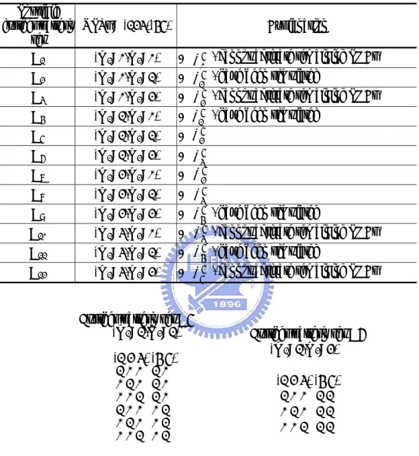
(24) Table 3.1. All possible pattern sets. Possible further pattern UPSs = (123)(45) set ∈ A1 (m1=0,m2=0) ∈ A2 (m1=0,m2=1) A3. (m1=0,m2=2). A4. (m1=1,m2=0). A5. (m1=1,m2=1). A6. (m1=1,m2=2). A7. (m1=2,m2=0). A8. (m1=2,m2=1). A9. (m1=2,m2=2). A10. (m1=3,m2=0). A11. (m1=3,m2=1). A12. (m1=3,m2=2). θ 05 θ15 ∈ θ5 2 ∈θ5 1 ∈ θ 25 ∈ θ5 3 ∈ θ 25 ∈ θ5 3 ∈ θ 45 ∈ θ 35 ∈ θ 45 ∈ θ5 5. Explanation , cannot activate remaining POEs , have been simulated , cannot activate remaining POEs , have been simulated. , have been simulated , cannot activate remaining POEs , have been simulated , cannot activate remaining POEs. Further pattern set A5 (m1=1,m2=1). Further pattern set A6 (m1=1,m2=2). (1 2 3) (4 5) 100 10 010 10 001 10 100 01 010 01 001 01. (1 2 3) (4 5) 100 11 010 11 001 11. Figure 3.2. Possible further pattern sets in A5 and A6. Note that A2 and A4 are ∈ θ15 as well as A9 and A11 are ∈ θ 45 . They have already been simulated before, thus, they are skipped from further verification pattern sets. Furthermore, A1, A3, A10, and A12 have the same logic assignments in each group. They cannot be the verification pattern sets either. Consequently, the remaining verification 16.

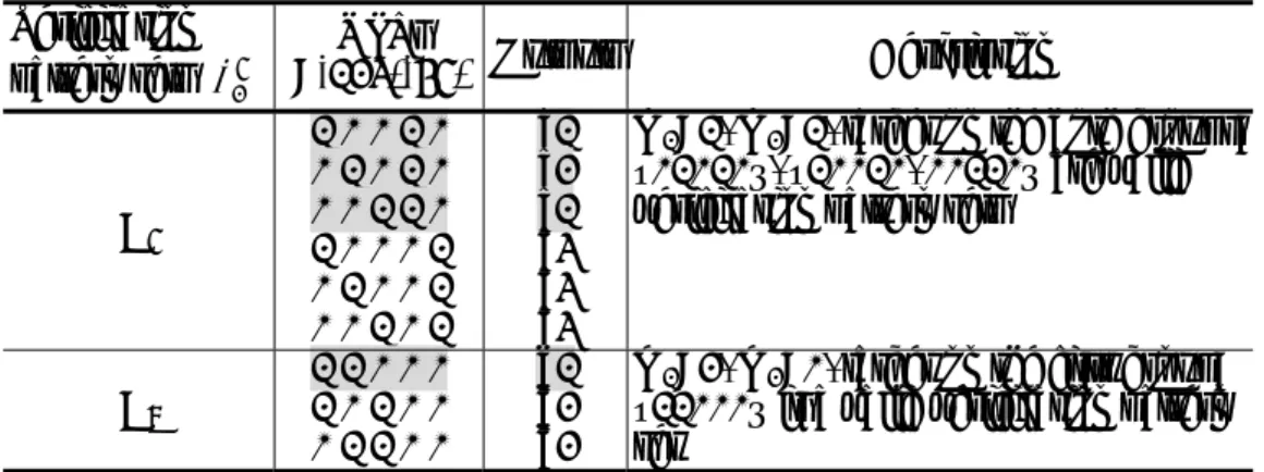
(25) pattern sets are A5 ~ A8, which are ∈ θ 25 and θ 35 respectively. We can choose only θ 25 , 5 or θ 35 , or both θ 2 and θ 35 for further verification sets since they all activate the. remaining EPSs and have the same opportunity to reduce the UPSs. To reduce the complexity of pattern generation, we choose one θ m5 at a time. In this example, either. θ 25 or θ 35 . Table 3.2 shows the selected verification patterns of θ 25 and their corresponding outputs which are represented in symbolic output representation. For example, the pattern set A5 contains six patterns, {10010, 01010, 00110, 10001, 01001, 00101} and their outputs are a1, a2, a1, a3, a3, and a3, respectively. The patterns in A5 can be grouped into three groups {10010, 00110}, {01010}, and {10001, 01001, 00101} according to their outputs. To select a group of patterns as the valid verification patterns, we always choose the group with the smaller size if it indeed can detect new EPS. Thus, in this example, {01010} and {10010, 00110} are selected as the valid verification patterns. When we apply these patterns {01010}, {10010, 00110} to verify the interconnections, we expect the outputs to be a2 and a1, respectively. If the real outputs are not a2 and a1, then the misplaced interconnects are detected. For the same reason, the gray patterns in A7 can be the valid verification patterns. After having these valid verification patterns, we have to figure out what new EPSs are detected and determine the remaining UPSs for further pattern generation.. 17.

(26) Table 3.2. θ 25 pattern sets. Verification pattern sets θ 25. A5. A7. UPSs Description =(123)(45) Outputs 10010 a1 m1=1, m2=1, target on the both groups; 01010 a2 {01010}, {10010, 00110} are valid 00110 a1 verification pattern sets 10001 a3 01001 a3 00101 a3 11000 b1 m1=2, m2=0, target on the first group; 10100 b2 {11000} is a valid verification pattern 01100 b2 set. The UPSs_Calculation stage is achieved by the proposed graph automorphism algorithm. Thus, we first introduce this algorithm, then apply it on the UPSs_Calculation.. 3.2. Graph Automorphism Algorithm The Graph Automorphism (GA) problem is a well-known and well- studied problem. However, it is not known to be either in P or NP-complete [2, 4]. Here we propose a heuristic to solve the GA problem.. Definition 3.3 : A graph G(V,E) with n vertices and m edges consists of a vertex set V(G)={V1,…,Vn} and an edge set E(G)={E1,…,Em}. Each edge consists of two vertices called its endpoints. (U,V) is an edge with endpoints U and V. A graph is undirected if there is no ”direction” on the edges. A graph is weighted if there are positive integer weights on the edges. The weight of the edge (U,V) is denoted as W((U,V)).. 18.

(27) 1. 2. 1. 2. 4. 3. 3. 4. 3. 4. 2. 1. Aut(G) (1). Aut(G) (2). Figure 3.3. An example of graph G and its automorphisms.. Definition 3.4 : An automorphism of graph G is a permutation of V(G) that preserves adjacency [20]. The automorphisms of G is denoted as Aut(G), and the cardinality of this set of automorphisms is denoted as |Aut(G)|.. Example 3.3: An undirected graph G = (V, E) as shown in Fig. 3.3 has V = {1,2,3,4} and E = {(1,2), (2,3), (3,4)}. Its automorphisms are also shown in Fig. 3.3 which are {1234 ,4321}, and |Aut(G)| = 2.. Definition 3.5 : A graph G is disconnected if we can partition its vertices into at least two nonempty sets, R and S, such that no vertex in R is adjacent to any vertex in S. That is, G is the disjoint union of the two subgraphs induced by R and S.. Definition 3.6 : For any two sets π1 and π2, its intersection π1∩π2 is a set that contains elements in both sets. We propose an automorphism representation that is similar to the UPS representation mentioned in Chapter 2.2 to record the automotphisms of a graph G. Vertices in the same group in this automorphism representation imply that any permutation of these vertices is an automorphism.. Example 3.4: For an automorphism representation π1 = (12)(34). It contains 2! × 2! automorphisms and they are {1234, 1243, 2134, 2143}. If π2 = (2)(134), it contains 1! ×. 19.

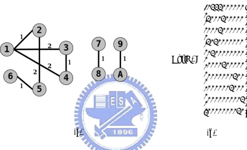
(28) 3! automorphisms and they are {1234, 1243, 3214, 3241, 4213, 4231}, then π1∩π2 = {1234, 1243}, which can be expressed as (1)(2)(34) in automorphism representation. Now, there are four steps in finding Aut(G) in our algorithm. Given an undirected graph G with N vertices, the initial automorphism representation is expressed as (123…N).. G: 1. 2 2. 1 2. 6 1. 2. 7. 3. 9 1. 1. 8. 4. 1. A. 5. (a). 0111000000  1000100000    0001000000    1010000000  0100000000  Adj(G) =   0000100000  0000000100    0000001000  0000000001    0000000010  (b). Figure 3.4. An undirected graph G and its Adj(G).. Step 1(Disjoint Graph - DG): If the graph is composed by t disconnected subgraphs, then the automorphism representation is divided into t groups such that each group corresponds to one subgraph. If the graph exists two or more subgraphs with the same number of vertices, then merge the corresponding subgroups into one. Since swapping any two vertices coming from disconnected subgroups with different size cannot be an automorphism, we can divide the automorphism representation of G respect to the graph connectivity of different sizes directly.. Example 3.5: Given a graph G as shown in Fig. 3.4(a). The graph G can be divided into three subgraphs. Since the subgraphs induced by vertices 7 and 8, and by vertices 9. 20.

(29) and 10 are the same size, therefore, by Step 1, the updated automorphism representation. π1= (123456)(789A). That means any vertex exchanged from these two groups cannot be an automorphism.. Definition 3.7 : The Degree Vector (DV) of a graph is a vector that contains each vertex’s degree such that DV[i] = degree of the ith vertex.. Step 2(Degree Vector - DV): Calculate the DV of the graph G. Then group the vertices with the same degrees into one group. Since exchanging of two vertices with different degrees cannot be an automorphism, we calculate the degree of each vertex and group the vertices with the same degrees into the same group. The grouping results are the automorphisms and are complied with the proposed automorphism representation. An automorphism has to satisfy the properties described in Step 1 and Step 2, so the updated automorphisms can be obtained from the intersection of automorphisms derived by Step 1 and Step 2.. Example 3.6: From Fig. 3.4(a), the DV of G is 5 3 3 3 3 1 1 1 1 1. By grouping the degree of each vertex, the automorphism representation is π2 = (1)(2345)(6789A). Thus, the updated automorphism representation by the intersection of Step 1 and Step 2 is π3 = (1)(2345)(6)(789A) which comes from (123456)(789A)∩(1)(2345)(6789A).. Definition 3.8 : The partial vector (PV) of vertex Vi in G is the ith row of adjacency matrix of G, Adj(G).. Definition 3.9 : A single element group (SEG) is a group that contains only one vertex in the automorphism representation. If updated automorphism representation contains SEG, go to Step 3, otherwise go 21.

(30) to Step 4.. Step 3(Repeated Automorphism - RA): Grouping the partial vector of each SEG vertex and intersect this grouping result with the updated automorphism representation. If the updated automorphism representation has newly generated SEG, repeat Step 3, otherwise go to Step 4. Since the automorphisms do not relate to the vertex in SEG, partition the partial vector of SEG vertices can determine the automorphisms. That is, only the neighbors with the same degree to the SEG vertices can be swapped as automorphisms.. Example 3.7: In the updated automorphism representation π3(1)(2345)(6)(789A), there are two vertices, 1 and 6, in SEG, respectively. We have known that in Fig. 3.4(a), vertex 1 is connected to vertices 2, 3 and 4, but is not connected to vertex 5. Thus, vertex 5 is different to vertices 2, 3 and 4. Besides, the weight of (1,2) is different to the weight of (1,3) and (1,4). We can use partial vector V_1 to reduce (2345) to (2)(34)(5). So as targeting on vertex 1, the partial vector V1 is 0122000000. It can be seen from the 1st row of Adj(G). Its corresponding V1_g, is (156789A)(2)(34). Then π3∩V1_g = (1)(2)(34)(5)(6)(789A) = π4. We find that vertices 2 and 5 are new vertices in SEG. Therefore, we conduct Step 3 for vertices 2, 5 and 6. As targeting on vertex 6, the partial vector V6 is 0000100000, V6_g is (12346789A)(5). π4∩V6_g = (1)(2)(34)(5)(6)(789A) =. π5. As targeting on vertex 5, the partial vector V5 is 0200010000, V5_g is (1345789A)(2)(6). π5∩V5_g = (1)(2)(34)(5)(6)(789A) = π6. As targeting on vertex 2, the partial vectors V2 is 1000200000, V2_g is (1)(5)(2346789A), π6∩V2_g = (1)(2)(34)(5)(6)(789A) = π7. Now, no more new vertex in SEG is generated, then go to Step 4. 22.

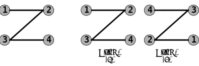
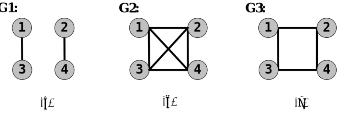
(31) Step 4: For the group with more than one element in it under automorphism representation, we observe its corresponding subgraph. If the subgraph is disconnected, give the joinder “. ”on those vertices which are connected, respectively. If the. subgraph is a cycle, then give the “ [ ] ” on these vertices. If the subgraph is a complete graph, then give the “ { } ” on these vertices. Observe those vertices in some subgraph under automorphism representation with just two elements in it. Record the partial vector if it really can reduce automorphism representation. After Step 1 ~ Step 3, we can assure that if more than one vertex in a group, they must have the same degrees and may be the combination of smaller subgraphs with the same number of vertices. Their corresponding subgraphs have three conditions. One is that it is just the combination of smaller subgraphs with same vertices, e.g. G1={(1,2), (3,4)} shown in Fig. 3.5(a). The number of |Aut(G1)| has special solution for it. We will introduce this in the next paragraph. Another condition is that it is a connected subgraph and is also a complete subgraph, e.g. G2={(1,2),(1,3),(1,4),(2,3),(2,4),(3,4)} shown in Fig. 3.5(b). So we can change the order of these vertices in the subgraph and remain identical under automorphism representation. The other condition is that it is a connected graph and it is a cycle shown, e.g. G3={(1,2),(1,3),(2,4),(3,4)} shown in Fig. 3.5(c). The number of |Aut(G3)| has special solution for it. We will also introduce this in the next paragraph. And if there are just two vertices in a subgraph, we have to observe the neighbors of these two vertices. If they have no neighbors in common, then the partial vectors of these two vertices are useful. Otherwise, the partial vectors of these two vertices are useless because these two vertices can be exchanged mutually.. 23.

(32) G1: 1. 2. G2: 1. 3. 4. 3. 2. G3: 1. 2. 4. 3. 4. (b). (a). (c). Figure 3.5. Disjoint graph, complete graph and cycle graph.. Example 3.8: For the updated automorphism representation π7 (1)(2)(34)(5)(6) (789A), there are six groups. Only the 6th group (789A) corresponds to the disconnected subgraph. Observe the vertices 7, 8, 9, and A, vertex 7 is connected with 8 while vertex 9 is connected with A. The group (789A) under automorphism representation now becomes ( 78 9 A ). Thus, the updated automorphism representation π7 is now (1)(2)(3 4)(5)(6) ( 78 9 A ). After Step 1 ~ Step 3, we can find the Aut(G) and |Aut(G) | can be obtained based on the updated automorphism representation. For updated automorphism representation. ( a1 a 2 L a nk )(b1b2 Lbnk ) ··· ( r1r2 L rnk ) , the |Aut(G)| = (n1!) × (n2!) × ··· × (nk!). If the joinders. are. shown. in. the. automorphism. representation,. such. as. ( a1 a 2 L a n1 b1b2 L bn1 L r1 r2 L rn1 ) , |Aut(G)| = {(n1!) × (n1!) × ··· × (n1!) × (the number of joinder)!}. For example in Fig. 3.5(a), Aut(G1)={1234, 1243, 2134, 2143, 3412, 4312, 3421, 3421}. |Aut(G1)| = 2! × 2! × 2! = 8. If the braces are shown in the automorphism representation, such as ({ a 1 a 2 L a n1 }), |Aut(G)| = n1!. For example in Fig. 3.5(b), Aut(G2)={1234, 1243, 1324, 1342, 1423, 1432, 2134, 2143, 2314, 2341, 2413, 2431, 3124, 3142, 3214, 3241, 3412, 3421, 4123, 4132, 4213, 4231, 4312, 4321}. 24.

(33) C 2n. |Aut(G2)| = 4! = 32. If the square brackets are shown in the automorphism representation, such as ([ a1 a 2 L a n1 ]), |Aut(G)| = (n1) × 2. For example in Fig. 3.5(c), Aut(G3)={1234, 1324, 2143, 2413, 3142, 3412, 4231, 4321}. |Aut(G3)| = 4 × 2 = 8. For this example, the updated automorphism representation π7 is (1)(2)(34)(5)(6) ( 78 9 A ). Thus, |Aut(G)| = 1! × 1! × 2! × 1! × 1! × (2! × 2! × 2!) = 16. We can enumerate these 16 automorphisms explicitly and they are {123456789A, 12345678A9, 123456879A, 12345687A9, 1234569A78, 123456A978, 1234569A87, 123456A987, 12435678 9A, 12435678A9, 124356879A, 12435687A9, 1243569A78, 124356A978, 1243569A87, 124356A987}.. 3.3. UPSs Calculation with Automorphism Technique From Chapter 3.1, we get the verification pattern sets. Now, we conduct the UPSs_Calculation stage with the graph automorohism (GA) technique to determine the remaining UPSs. For the example in Fig. 3.6(a), we assume the verification pattern set S1 has four patterns P1, P2, P3 and P4. To solve the problem of calculating the remaining UPSs of the pattern set S1 with n bits, an undirected, weighted graph G(V,E) is constructed, which corresponds to the set S1 with |S1| patterns, P1 to P|S1| . Pi[j] in S1 denotes the jth bit in Pi where i = 1 ~ |S1| and j = 1 ~ n. The vertex Vk in G corresponds to the kth input variable/port in S1. For all patterns P1 to P|S1| in S1, when Pi [k] = Pi [k’] = 1, an edge VkVk’ is added into G and W(VkVk’)=1 where (k, k’) are all C2n bit pairs. If the edge VkVk’ has existed in G,. 25.

(34) W(VkVk’) is increased by one.. Example 3.9: For P1[1 : 7] in S1 shown in Fig. 3.6(a), 1010001, since P1[1] = P1 [3] = P1 [7] = 1, edges V1V3, V1V7, and V3V7 are added into G, respectively. For P2[1 : 7], 0100110, edges V2V5, V2V6, and V5V6 are added into G, respectively, and so on. The constructed graph G is an undirected weighted graph and is shown in Fig. 3.6(b). Its corresponding adjacency matrix, Adj(G), is shown in Fig. 3.6(c). In Adj(G), if there is no edge between Vk and Vk’ in G, Adj(G)[k][k’] = Adj(G)[k’][k] = 0; otherwise Adj(G)[k][k’] = Adj(G)[k’][k] = W(VkVk’). The problem of calculating the remaining UPSs in S1 is now transformed to finding all automorphisms of G. The effectiveness of this problem transformation is that the position relations of digit 1s in each pattern in S1 are transformed to the connectivity relations in G. Finding the port misplacements that maintain S1 to be invariant (calculating UPSs) is equivalent to finding all automorphisms of G.. 1 Verification pattern set S1 (1 P1[1:7]=1 P2[1:7]=0 P3[1:7]=0 P4[1:7]=0. 2 0 1 0 0. 3 1 0 1 0. 4 0 0 1 0. 5 0 1 0 1. 6 0 1 0 1. 7 ) 1 0 1 1. 2. 1. 1 2. 7 1. 3. 1. 1. 1. 6. 1. 1. 4. 2. 0010001  0000110    1001002  Adj(G) = 0010001    0100021    0100201  1021110   . 5 (a). (b). Figure 3.6. UPSs_Calculation with GA technique.. 26. (c).

(35) We demonstrate the UPSs_Calculation stage by the proposed GA algorithm using the following example. The initial UPSs is π0 = (1234567). In Step1, the graph in Fig. 3.6(b) is a connected graph and cannot be divided into subgraphs. Thus, the UPS remains unchanged. In Step 2, the degree vector DV[1:7] is 2 2 4 2 4 4 6. It groups the three 2s in one group, three 4s in another group, and one 6 in the third group. The grouped results can be represented as (222)(444)(6) and its corresponding UPSs are (124)(356)(7). Then the updated UPS π1 = π0∩(124)(356)(7) = (1234567)∩(124)(356)(7) = (124)(356)(7). In Step 3, there is one SEG vertex 7. As targeting on vertex 7 in updated UPSs π1, the partial. vector. V7. is. 1021110,. V7_g,. (1456)(27)(3).. Then. π2 =. π1∩V7_g. =(14)(2)(3)(56)(7). SEGs of vertices 2 and 3 are newly generated. Therefore, we have to repeat Step 3 for vertices 2 and 3, respectively. As targeting on vertex 2, the partial vector V2 is 0000110, V2_g is (12347)(56). π3 = π2∩V2_g = (14)(2)(3)(56)(7). As targeting on vertex 3, the partial vector V3 is 1001002, V3_g is (14)(2356)(7). π4 =. π3∩V3_g = (14)(2)(3)(56)(7). Now, no new vertex in SEG is generated, Step 3 is terminated. For the updated UPS π4 (14)(2)(3)(56)(7), there are five groups. The partial vector of the first group and the 4th group is useless because the neighbors of each group are the same. Thus, the updated UPS π4 remains unchanged. The GA technique is now finished. The summary of this example is shown in Fig. 3.7.. 27.

(36) Initial UPSs (1 2 3 4 5 6 7) Step (1) DG : (1 2 3 4 5 6 7). (1 2 3 4 5 6 7). Step (2) DV : (1 2 4)(3 5 6)(7). (1 2 4)(3 5 6)(7) new isolated vertex (7). Step (3) RA: Target on 7 PV : (1 4 5 6)(2 7)(3). (1 4)(2)(3)(5 6)(7) new isolated vertices (2)(3). Target on 2 PV : (1 2 3 4 7)(5 6) Target on 3 PV : (1 4)(2 3 5 6)(7). (1 4)(2)(3)(5 6)(7) (1 4)(2)(3)(5 6)(7). Figure 3.7. Graph Automorphism (GA) technique. In the same example, the remaining UPSs obtained from the CV approach are (124)(356)(7) and from the SAA approach are (124)(3)(56)(7) in [19]. However, it can be further reduced to (14)(2)(3)(56)(7) by the GA approach and the real remaining UPSs are (14)(2)(3)(56)(7). These results demonstrate that the GA approach gets more precise remaining UPSs than that of the CV approach and the SAA approach. In this example in Fig. 3.7, Step 4 seems useless for reducing UPSs. However, it also provides information for reducing UPSs later on. Hence we do not conduct Step 4 actually in the AVPG for preserving the UPS representation concisely. But its impact on reducing UPSs is still remained by using partial vector concept.. Definition 3.10: The partial vector of vertex t is called automorphism message of t, denoted as AM_t, if vertex t does not belong to SEG in the UPS representation. Giving UPSs (1234)(56)(78)(9A)(BC), assume that the valid verification pattern set is {10010101010, 010010100101, 001001011010, 000101010101}, as shown in Fig.. 28.

(37) 3.8(a) and its adjacency matrix is shown in Fig. 3.8(b). If we apply the GA technique of Step 1 ~ Step 3, we can find that the updated UPS is still (1234)(56)(78)(9A)(BC). Then we keep this verification pattern set and calculate AM for each vertex t. For example, AM_1 defined as the partial vector of vertex 1 is 000010101010, AM_C defined as the partial vector of vertex C is 010111110200 and they are shown in Fig. 3.8(c). AM_1 implies that if vertex 1 is in SEG after some iteration later, the vertices 5, 7, 9, 11 (vertices with assignment 1 in AM_1) can also be in SEGs as well. Thus if we assume vertex 1 in SEG indeed in the next UPSs_Calculation process, then we can reduce UPSs from (1234)(56)(78)(9A)(BC) to (1) (234)(5)(6)(7)(8)(9)(A)(B)(C) according to AM_1. Other AMs have the similar effect on reducing UPSs.. Verification pattern set (1234)(56)(78)(9A)(BC) 1000 10 10 10 10 0100 10 10 01 01 0010 01 01 10 10 0001 01 01 01 01. Adj(G) =. (a) AM_1:. 000010101010. 000010101010 000010100101 000001011010 000001010101 110000201111 001100021111 110020001111 001102001111 101011110020 010111110002 101011112000 010111110200. AM_C: 010111110200 (b). (c). Figure 3.8. Verification pattern set with automorphism message (AM). Now, the complete AVPG Flow with graph automorphism (GA) technique is shown in Fig. 3.9, where DG means Disjoint Graph in Step 1, DV means Degree Vector in Step 2, RA means the Repeated Automorphism in Step 3, and AM means Automorphism Message in Step 4. The pseudo code of AVPG with GA technique is 29.

(38) shown in Fig. 3.10. In line 7, 9, it generates patterns and the output simulation in line 11. The effectiveness of the simulated patterns is determined in line 12. The steps of GA technique are in line 14 ~ 16, 20, 23, respectively. In line 17, 21, it includes the valid patterns into the verification pattern set. At the end of the algorithm, the verification pattern set, error coverage and UPSs are returned.. Start. E_C = 0, Iteration = 0. E_C = 100% or Iteration > bound. Yes. No. Pattern_Generation. Pattern_Simulation. Get_Valid_Patterns. UPSs_Calculation (DG+DV+RA+AM) (Keep useful AM) Iteration ++. Figure 3.9. Complete AVPG flow.. 30. Stop.

(39) Algorithm: Automatic Verification Pattern Generation with Automorphism Technique Input: CUV ( N-input, M-outtput ) Output: Verification Pattern set (Veri_P_S) , error coverage (E_C) , UPS { 01 variable i Å 0; 02 UPS Å (1 2 3 ... N) ; 03 E_C Å 0; 04 simulated[N-1] Å {0,0, ... ,0} ; 05 Veri_P_S Å {φ} ; 06 Temp_P_S Å {φ } ; do { 07 08. if (i==0) {. N N verification patterns Å C1 , C N −1 i Å i+1;. ;. 09. } else verification patterns Å Pattern_generation (UPS , simulated[N-1]) ;. 10 11 12 13 14 15 16. Update (simulated[N-1]); outputs Å Simulation (verification patterns); {valid verification patterns} Åoutput_analysis(outputs); G(V,E) Å Transition ({valid verification patterns }) ; {UPS_tmp} ÅDG ( G , UPS) ; {UPS_tmp} ÅDV ( G , UPS_tmp) ; {UPS_tmp} ÅRA ( G , UPS_tmp) ;. 17 18 19 20. 21 22 23. if ( UPS_tmp ≠ UPS ) { Veri_P_S Å Veri_P_S ∪ {valid verification patterns } ; E_C Å E_C_calculation (UPS_tmp) ; } UPS Å UPS_tmp ; UPS_tmp2 Å Use_AM (Temp_P_S,UPS) ; if ( UPS_tmp2 ≠ UPS ) { Veri_P_S Å Veri_P_S ∪ Temp_P_S ; UPS Å UPS_tmp2 ; } {Temp_P_S} Å Keep_AM (G,UPS); if (E_C == 1) break ; if (simulated[N-1]=={1,1, ... ,1}) break ;. 24 }. } while (E_C !=1 ) ; return (Veri_P_S , E_C , UPS) ;. Figure 3.10. Pseudo code of AVPG with GA technique.. 31.

(40) Chapter 4 Experimental Results The GA-based algorithm is implemented in Programming Language Interface (PLI) environment. Experiments are conducted over a set of ISCAS-85 and some MCNC benchmarks with large number of inputs. The benchmarks are in Verilog HDL format. Since only the simulation information of these benchmarks is needed to conduct the experiments, arbitrary levels of design description can be used for generating verification pattern set. Table 4.1 summarizes the experimental results of the comparison of SAA approach in [19] and our graph automorphism technique algorithm of AVPG. The first five columns show the parameters of each benchmark, including name, |PI|, |PO|, the number of literals (lits.) and the number of POEs. The |PI| 32.

(41) represents the number of inputs and the size of the POEs set is |PI|!-1. The |PO| represents the number of outputs and influences on the probability of error effect propagation. The number of literals indicates the complexity of a benchmark. The remaining columns show the number of verification patterns (pats.), error coverage (E_C) and the CPU time. The error coverage is defined as 1- (# of undetected POEs / # of all POEs). The ratio is defined as (the patterns of GA approach / the patterns of SAA approach). The iteration bound is set to 100. The CPU time is measured in second on a Sun Sparc II Workstation. The algorithm will be terminated automatically if iterations are over the bound or the error coverage reaches 100%, and the verification pattern set and the error coverage are returned. For example, in c880 benchmark, the number of verification patterns is decreased from 130 to 73 and the ratio of pattern size is 0.56. We can see that for most circuits, the number of verification patterns is reduced by the proposed techniques – a new pattern generation algorithm and the GA technique. Furthermore, the CPU time is acceptable.. 33.

(42) Table 4.1. Comparisons on experimental results of SAA approach and GA approach. Bench c17 c880 c1355 c1908 c432 c499 c3540 c5315 c2670 c7552 c6288 des alu4 apex6 i9 i8 i7 i6 i5 rot x3 x4 pair Total Ratio. Parameters |PI| |PO| Lits. 5 2 12 60 26 703 41 32 1032 33 25 1497 36 7 382 41 32 616 50 22 2934 178 123 4369 233 140 2043 207 108 6098 32 32 4800 256 245 7412 14 8 1278 135 99 904 88 63 1453 133 81 4626 199 67 1311 138 67 1037 133 66 556 135 107 1424 135 99 1816 94 71 1040 173 137 2667. SAA approach Pats. E_C(%) Pats. 5 100 4 130 99.999 73 51 100 39 45 100 41 35 100 35 40 100 37 89 100 70 222 100 174 351 99.999 237 448 99.999 312 30 99.999 30 255 100 255 17 100 14 187 99.999 154 107 100 92 204 100 156 240 100 194 138 100 130 133 100 125 247 99.999 150 165 99.999 145 141 99.999 117 186 100 120 3466 2704 1 0.78. 34. GA approach E_C(%) Time(s) 100 0.23 99.999 5.59 100 0.91 100 0.93 100 0.41 100 0.72 100 10.70 100 53.42 99.999 92.71 99.999 87.45 99.999 2.84 100 5.47 100 0.51 99.999 12.88 100 1.12 100 13.65 100 12.77 100 10.12 100 10.65 99.999 17.40 99.999 9.34 99.999 5.14 100 21.38. Ratio 0.80 0.56 0.74 0.91 1 0.93 0.75 0.78 0.67 0.69 1 1 0.82 0.82 0.86 0.76 0.81 0.94 0.94 0.61 0.88 0.83 0.65.

(43) Chapter 5 Applications We use this graph automorphism-based algorithm for computing maximal sets of symmetric inputs of circuits. It can be used to identify nonsymmetric inputs in a circuit and enhance the efficiency of input matching, library binding (technology mapping), as well as logic verification problems.. 5.1. About Symmetric Two inputs xi an xj of a single/multi-output logic function f(X) are said to be symmetric, if exchanging xi and xj does not change f, i.e., f(x1…, xi,…, xj,…xn) = f(x1,…, xj,…, xi,…, xn)[34]. 35.

(44) Symmetric input sets of a logic function are subsets of inputs such that any permutation of the inputs within a subset leaves the function invariant [33, 34]. The problem of finding maximal symmetric input sets is formulated as following [33, 34]: Given a single/multi-output function f(X), find maximal subsets of inputs X1, X2, …, Xk ⊆ X, such that X1 ∪ X2 ∪ … ∪Xk = X and the inputs in every subset Xi can be. permuted in any fashion without changing the function. The symmetry relation is an equivalence relation, and the maximal symmetric input sets are its equivalence classes. To find the maximal symmetric input sets, it is therefore sufficient to find all pairs of symmetric inputs and then take the unions of all the pairs having nonempty intersection. This symmetry is known as the classical symmetry or the nonskew nonequivalence symmetry [35]. The definition of this symmetry translates into the following requirements for the cofactors of function f Xi Xj = f Xi Xj with respect to any two inputs xi and xj. Symmetric input sets, and the particular maximal symmetric input sets, are important in problems of design verification and diagnosis [12, 21, 23, 25-27, 29-32, 40-44] and in problems of technology mapping, where it is required to find a library macro to implement a given logic block [24, 28, 36, 39]. The goal of design verification is to check whether a given implementation follows the specification for which it was designed. If implementation is incorrect, diagnosis may be used for gate-level implementations [12, 25, 29-31, 40, 41] to locate and then correct the design. It is typically assumed that the correspondence between specification and implementation inputs is known. However, due to design errors, implementation inputs may be interchanged, and hence it may be necessary to compute the actual. 36.

(45) correspondence between specification and implementation inputs. This problem was studied in [12], where it was observed that finding the symmetric input sets can save the effort of trying different permutations of inputs belonging to the same symmetric set, since all these permutations are equivalent. In technology mapping applications [24, 28, 36, 39], it is required to check whether a logic block in the given circuit exists in a macro library. The problem that arises is to find a correspondence between the inputs of the logic block and the inputs of a library macro and a correspondence between the outputs of the logic block and the outputs of the library macro, such that under the two correspondences the library macro is logically equivalent to the logic block. The library macro can then be used to implement the logic block. For this problem, too, finding the symmetric input sets of the logic block and the library macro can save the effort of trying different permutations of inputs belonging to the same symmetric set. The problem of finding maximal subsets of symmetric inputs has been studied for single-output functions, for which the set of all minterms that set the function to 1 is available (or can be derived) [33]. An efficient method to find subsets of symmetric inputs, applicable to large multi-output circuits, is studied here. In parallel to our work on this problem [35, 37, 38], methods using BDD’s [22] are investigated in [35, 37]. However, these BDD-based algorithms are not applicable to the designs that described in behavior level or RT-level, e.g., soft Intellectual Property, or that do not have compact BDD representation. Thus, simulation-based approach [38] was proposed to compute the maximal sets of symmetric inputs. [38] establishes two steps to accomplish the input symmetric identification. The first step uses heuristic to identify inputs that do not 37.

(46) belong to the same symmetric input set. Although the signature-based heuristic used in [24, 36, 39] can be used for this purpose, the heuristics in [24, 36, 39] were applied to circuits having compact BDD representation. The second step uses test generation techniques to further identify the inputs that were not distinguished by the heuristic. The efficiency of [38]-like approach for computing the maximal sets of symmetric inputs in circuits without compact BDD representation depends on the “ability” of heuristics. Good heuristics can distinguish more nonsymmetric inputs prior to entering computation intensive test generation step. Thus, we focus on the first step of [38]-like approach by using graph automorphism-based heuristic.. 5.2. Symmetric with GA Algorithm We exchange the UPS representation to the Symmetric-ASymmetric Inputs (SASIs) to represent the maximal symmetric inputs sets. For an N-input circuit, we number its inputs from 1 to N. Initially, we assume that all inputs are symmetric, the corresponding SASIs representation is (1 2 3 … N), i.e., all inputs are placed in one group. If we claim that input i is asymmetric to the other inputs by our methods, the input i is isolated from original group and can be expressed as (i)(1 2 … i-1 i+1 … N). Please note the order of the groups in the SASIs representation is irrelevant, neither is the order of the number in each SASIs group. By the SASIs representation, if any two inputs are not placed in the same group, then they are nonsymmetric inputs. Otherwise they are “possibly” symmetric. Obviously, according to SASIs representation, we can realize exactly which inputs are asymmetric to the other inputs. Thus, further efforts ought to be put onto the groups that contain undistinguished inputs. The following example demonstrates the 38.

(47) details of the SASIs representation. Given an 8-input circuit, the inputs are numbered from 1 to 8. The SASIs representation (12345678) represents all inputs are symmetric. The SASIs representation (125)(4)(3678) indicates that inputs 1, 2 and 5 are symmetric and inputs 3, 6, 7 and 8 are symmetric. Input 4 is the only one element in the second group. It means that input 4 is asymmetric to the other inputs. The SASIs (125)(4)(3678) can also be expressed as (4)(215)(8763). The SASIs representation (1)(2)(3)(4)(5)(6)(7)(8) has eight groups and each group has only one element; therefore, these inputs are nonsymmetric inputs. The goal of the proposed heuristic is to induce SASIs representation from (12345678) to (1)(2)(3)(4)(5)(6)(7)(8) if these inputs are asymmetric indeed. Then, we change the AVPG to Automatic Computing Symmetric Procedure (ACSP). Its flow chart is shown in Fig. 5.1. This flow chart is similar to the AVPG flow shown in Fig. 3.8. The ACSP reads a combinational circuit and generates heuristic patterns. The patterns simulation results provide information to SASIs_Calculation stage for figuring out nonsymmetric inputs in SASIs representation. Then further heuristic patterns are generated according to the updated SASIs in the next iteration. When all inputs are identified as nonsymmetric or the iterations are over the bound, the ACSP will be terminated and the maximal symmetric input sets are returned. The pseudo code of ACSP with GA technique is shown in Fig. 5.2. In line 5, 7, it generates patterns and the output simulation in line 9. The valid generated pattern sets are determined in line 10. The steps of GA technique are in line 11 ~ 17. At the end of the algorithm, the SASIs are returned. 39.

(48) Start. Iteration = 0. All nonsymmetric or Iteration > bound. Yes. No. Pattern_Generation. Pattern_Simulation. SASIs_Calculation (DG+DV+RA+AM) (Keep useful AM) Iteration ++. Figure 5.1. Complete ACSP flow.. 40. Stop.

(49) Algorithm: Automatic Computing Symmetric Procedure with GA Technique Input: circuit ( N-input, M-output ) Output: SASI { 01 variable i Å 0; 02 SASI Å (1 2 3 ... N) ; 03 simulated[N-1] Å {0, 0, ... , 0} ; 04 Intending_AM Å {φ } ; do { if (i==0) { 05 generated pattern sets Å C1N , C NN−1 ; 06 i Å i+1; } else 07 generated pattern sets Å Pattern_Generation (SASI , simulated[N-1]) ; 08 09 10 11 12 13 14 15 16 17. 18 }. Update (simulated[N-1]) ; outputs Å Simulation (generated pattern sets) ; {valid generated pattern sets} Å outputs_analysis (outputs) ; G(V,E) Å Transformation ({valid generated pattern sets}) ; {SASI_tmp} Å DG ( G, SASI) ; {SASI_tmp} Å DV ( G, SASI_tmp) ; {SASI_tmp} Å RA ( G, SASI_tmp) ; {SASI_tmp} Å Use_AM (Intending_AM , SASI_tmp) ; SASI Å SASI_tmp ; {Intending_AM} Å Keep_AM (G , SASI); if (simulated[N-1]=={1,1,...,1}) } while (all nonsymmetric) ; return (SASI) ;. break ;. Figure 5.2. Pseudo code of ACSP with GA technique.. 5.3. Experimental Results The GA-based algorithm is implemented in Programming Language Interface (PLI) environment. Experiments are conducted over a set of ISCAS-85 and some MCNC benchmarks. Table 5.1 summarizes the experimental results of the previous approach in [38] and our GA-based algorithm. The first four columns show the parameters of each benchmark, including name, |PI|, |PO| and the number of literals (lits.). The |PI| 41.

(50) represents the number of inputs. The |PO| represents the number of outputs. The number of literals indicates the complexity of a benchmark. This number is derived from its gate level description. The remaining columns show the sets of inputs that cannot be distinguished. In fact, these input sets are possibly symmetric inputs sets. They are expressed by pairs (size, number of sets), where size is the size of an input set and the following is the number of sets of that size. For example, for c880, three sets of size two means that they are possible symmetric inputs and the other sets of size one means that the 54 inputs are asymmetric to other inputs. The iteration bound is set to 100. The CPU time is measured in second on a SUN Sparc II workstation. The algorithm will be terminated automatically if iterations are over the bound or all inputs are nonsymmetric, and SASIs are returned. According to Table 5.1, we can find that in previous approach, c499, c1355, and c1908 still have potentially symmetric input sets, but our approach can distinguish each input as a nonsymmetric input. Also for c2670 and c6288, our approach distinguishes more nonsymmetric inputs than that of [38]. Please note for c6288, our approach does not distinguish each input as a nonsymmetric input while [38] does. This is because our heuristic patterns inherently cannot distinguish each input of a multiplier such as c6288. [38] uses test generation technique to conquer it instead. Table 5.2 also shows the results on some MCNC benchmarks. Most nonsymmetric inputs are distinguished efficiently as usual for most benchmarks. These results demonstrate that our approach acts as a good filter to identify nonsymmetric inputs as many as possible in a circuit such that significant efforts can be saved for other succeeding applications. Our approach is applicable to sequential circuits if circuit states can be fully specified. The experiments on sequential circuits are progressing. 42.

(51) Table 5.1. Comparisons on experimental results of previous approach in [38] and GA approach. Bench. |PI| |PO| c17 c880 c1355 c1908 c432 c499 c3540 c5315 c2670 c7552 c6288. Previous approach in GA approach [38] (size, number of Time (size, number of Time Lits. sets) (s) sets) (s) 12 (1,5) 0.04 (1,5) 0.23 703 (1,54)(2,3) 2.86 (1,54)(2,3) 1.74 1032 (1,32)(9,1) 3.16 (1,41) 0.91 1497 (1,22)(5,1)(6,1) 1.81 (1,33) 0.93 382 (1,36) 0.24 (1,36) 0.41 616 (1,32)(9,1) 1.07 (1,41) 0.72 2934 (1,50) 19.52 (1,50) 10.70 4369 (1,178) 33.95 (1,178) 33.42 2043 (1,221)(2,2)(8,1) 59.95 (1,223)(2,2)(6,1) 42.55 6098 (1,166)(2,6)(3,1) 5514 (1,183)(2,8)(3,1) 191.33 (5,2)(4,4) (5,1) 4800 (1,32) 6.53 (2,16) 2.84. Parameters. 5 2 60 26 41 32 33 25 36 7 41 32 50 22 178 123 233 140 207 108 32. 32. 43.

(52) Table 5.2. Results of some MCNC benchmarks. Circuit 9symml b1 b9 cm138a cm162a cm163a cm82a cmb count frg1 lal pm1 term1 x1 x2 x3 x4 z4ml alu4 apex6 des i5 i6 i7 i8 i9 pair rot. |PI| 9 3 41 6 14 16 5 16 35 28 26 16 34 51 10 135 94 7 14 135 256 133 138 199 133 88 173 135. |PO| 1 4 21 8 5 5 3 4 16 3 19 13 10 35 7 99 71 4 8 99 245 66 67 67 81 63 137 107. Lits. 277 17 236 35 58 53 26 62 174 130 223 85 625 2141 71 1816 1040 77 1278 904 7412 556 1037 1311 4626 1453 2667 1424. 44. (size, number of sets) (9,1) (1,1)(2,1) (1,31)(2,5) (1,4)(2,1) (1,12)(2,1) (12,1)(4,1) (1,3)(2,1) (4,2)(8,1) (1,33)(2,1) (1,26)(2,1) (1,16)(2,5) (1,9)(3,1)(4,1) (1,32)(2,1) (1,49)(2,1) (1,8)(2,1) (1,133)(2,1) (1,92)(2,1) (2,2)(3,1) (1,14) (1,135) (1,256) (1,133) (1,138) (1,199) (1,133) (1,88) (1,173) (1,115)(2,5)(3,2)(4,1). Time(s) 0.95 0.24 3.88 0.29 0.37 0.36 0.39 0.98 0.58 0.41 1.87 0.31 0.48 20.97 0.49 9.37 5.14 0.77 0.51 12.88 5.47 10.65 10.12 12.77 13.65 1.12 21.38 17.4.

(53) Chapter 6 Conclusions In the SoC era, the embedded cores are mixed and integrated to create a system chip. The verification of the core-based system design should be focused on how the cores communicate with each other. However, before the interface verification, the interconnections between the cores in an SoC have to be verified first. System integrators integrate those cores manually and have the possibility of incorrect integration due to the misplaced I/O ports. Therefore, we adopt the connectivity-based POE model to raise the abstraction level of the design verification and to reduce the time on functional verification in core-based design methodology. In this thesis, we present a new pattern generation algorithm to activate all 45.

(54) remaining POEs and the GA technique to improve the UPSs_Calculation procedure. These two approaches get more precise remaining UPSs and therefore accelerate the AVPG and generates a more efficient verification pattern set for verifying core-based designs. Besides, we use this GA technique for computing maximal sets of symmetric inputs of circuits. It can be used to identify nonsymmetric inputs in a circuit and enhance the efficiency of input matching, library binding (technology mapping), as well as logic verification problems. The experimental results demonstrate that our approach distinguishes more nonsymmetric inputs than that of previous work.. 46.

(55) References [1]. M. Abramovici, M. A. Breuer, and A. D. Friedman, “Digital Systems Testing and Testable Design,” Computer Science Press, 1990, pp. 95.. [2]. M. Agrawal and V. Arvind, “A Note on Decision Versus Search for Graph Automorphism,” in Eleventh Annual IEEE Conference Computational Complexity, 1996, pp. 272–277.. [3]. H. Chang, L. Cooke, M. Hunt, G. Martin, A. McNelly, and L.Todd, Surviving the SOC Revolution—A Guide to Platform-Based Design. Norwell, MA: Kluwer, 1999.. [4]. R. Chang, W. Gasarch, and J. Toran, “On Finding the Number of Graph Automorphism,” in IEEE Structure in Complexity Theory Conference, 1995, pp. 288–298.. [5]. D. I. Cheng and M. Marek-Sadowska, “Verifying Equivalence of Functions with Unknown Input Correspondence,” in Proceedings European Design Automation Conference (EDAC), 1993, pp. 81-85.. [6]. K.-T. Cheng, and J.-Y. Jou, ”A Functional Fault Model for Sequential Machines,” IEEE Transactions on Computer-Aided Design, Sep. 1992, pp.1065-1073.. [7]. P. Goel and M. T. McMahon, “Electronic Chip-in-place Test,” in Proceedings IEEE International Test Conference, Oct. 1982, pp. 83–90.. [8]. A. Hassan, V. K. Agarwal, B. Nadeau-Dostie, and J. Rajski, “BIST of PCB Interconnects Using Boundary-scan Architecture,” IEEE Transactions Computer-Aided Design, Oct. 1992, pp. 1278–1288.. [9]. H.-T. Liaw, J.-H. Tsaib and C.-S. Lin, “Efficient Automatic Diagnosis of Digital Circuits,” International Conference On Computer-Aided Design, Nov. 1990, pp.464-467.. [10]. J. C. Madre, O. Coudert and J. P. Billon, “Automating the Diagnosis and the Rectification of Design Errors with PRIAM,” in Proceedings International Conference on Computer-Aided Design, Nov. 1989, pp. 30-33.. [11]. J. Mohnke and S. Malik, “Permutation and Phase Independent Boolean Comparison,” in Proceedings European Design Automation Conference (EDAC), 1993, pp. 86-92.. [12]. I. Pomeranz and S. M. Reddy, “On Diagnosis and Correction of Design Errors,” in Proceedings International Conference On Computer-Aided Design, Nov 1993.. R-1.

(56) [13]. J. A. Rowson and A. Sangiovanni-Vincentelli, “Interface-Based Design,” in Proceedings Design Automation Conference, June 1997, pp. 178–183.. [14]. U. Schlichtmann, F. Brglez and M. Hermann, “Characterization of Boolean Functions for Rapid Matching in EPGA Technology Mapping,” in Proceedings Design Automation Conference, June 1992, pp. 374-379.. [15] M. H. Schulz, E. Trischler, and T. M. Sarfert, ”SOCRATES: a Highly Efficient Automatic. Test. Pattern. Generation. System,”. IEEE. Transactions. on. Computer-Aided Design, Jan. 1988, pp.126-137. [16]. K.A. Tamura, “Locating Functional Errors in Logic Circuits,” in Proceedings Design Automation Conference, 1989, pp. 185-191.. [17]. S.-W. Tung and J.-Y. Jou, “A Logic Fault Model for Library Coherence Checking,” Journal of Information Science and Engineering, Sept. 1998, pp. 567–586.. [18]. C.-Y. Wang, S.-W. Tung, and J.-Y. Jou, “On Automatic-verification Pattern Generation for SoC with Port-order Fault Model,” IEEE Transactions on Computer-Aided Design, vol. 21, Apr. 2002, pp. 466–479.. [19]. C.-Y. Wang, S.-W. Tung, and J.-Y. Jou, “An Automorphic Approach to Verification Pattern Generation for SoC Design Verification Using Port-Order Fault Model,” IEEE Transactions on Computer-Aided Design, vol. 21, Oct. 2002, pp. 1225–1232.. [20]. D. B. West, ”Introduction to Graph Theory,” Upper Saddle River, New Jersey, Prentice-Hall, Incorporation, 1996.. [21]. M. S. Abadir, J. Ferguson, and T. E. Kirkland, “Logic Design Verification via Test Generation,” IEEE Transactions on Computer, Jan. 1988, pp. 138-148.. [22]. R. E. Bryant, “Graph-based Algorithms for Boolean Function Manipulation,” IEEE Transactions on Computer, Aug. 1986, pp. 677-691.. [23]. P. Camurati and P. Prinetto, “Formal Verification of Hardware Correctness: Introduction and Survey of Current Research,” IEEE Computer, July 1988, pp. 8-19.. [24]. D. I. Cheng and M. Marek-Sadowska, “Verifying Equivalence of Functions with Unknown Input Correspondence,” in Proceedings of European Design Automation Conference (EDAC), 1993, pp.81-85.. R-2.

(57) [25]. P. Y. Chung and I. N. Hajj, “ACCORD: Automatic Catching and Correction of Logic Design Errors in Combinational Circuits,” in Proceedings of International Test Conference, 1992, pp. 742-751.. [26]. S. Devadas, H. K. T. Ma, and A. R. Newton, “On the Verification of Sequential Machinesat Differing Levels of Abstraction,” IEEE Transactions on Computer-Aided Design, June 1988, pp. 713-722.. [27]. J. Jain, J. Bitner, D. S. Fussell, and J. A. Abraham, “Probabilistic Design Verification,” in Proceedings of International Conference Computer-Aided Design, Nov. 1991, pp. 468-471.. [28]. K. Keutzer, “DAGON: Technology Binding and Local Optimization by DAG Matching,” in Proceedings of Design Automation Conference, 1987, pp. 341-347.. [29]. S. Y. Kuo, “Locating Logic Design Errors via Test Generation and Don’t-care Propagation,” in Proceedings of European Design Automation Conference (EDAC), Sep. 1992, pp. 466-471.. [30]. H. T. Liaw, J. H. Tsaih, and C. S. Line, “Efficient Automatic Diagnosis of Digital Circuits,” in Proceedings of International Conference Computer-Aided Design, Nov. 1990, pp. 464-467.. [31]. J. C. Madre, O. Coudert, and J. P. Billon, “Automating the Diagnosis and the Rectification of Design Errors with PRIAM,” in Proceedings of International Conference Computer-Aided Design, Nov. 1989, pp. 30-33.. [32]. F. Maruyama and M. Fujita, “Hardware Verification,” IEEE Computer, Feb. 1985, pp. 22-32.. [33]. E. J. McCluskey, “Detection of Group Invariance or Total Symmetry of a Boolean Function,” Bell System Tech, J., Nov. 1956, pp. 1445-1453.. [34]. E. J. McCluskey, Logic Design Principles with Emphasis on Testable Semicustom Circuits, Prentice-Hall, 1986.. [35]. Alan Mishchenko, “Fast Computation of Symmetries in Boolean Functions” IEEE Transactions on Computer-Aided Design of Integrated Circuits and Systems, Vol. 22, No. 11, Nov. 2003, pp. 1588-1593.. [36]. J. Mohnke and S. Malik, “Permutation and Phase Independent Boolean Comparison,” in Proceedings of European Design Automation Conference (EDAC), 1993, pp. 86-92.. R-3.