異質性投資人最適股利政策之研究

全文

(1)國立中山大學. 企業管理學系. 博士論文. 異質性投資人最適股利政策之研究 Optimal Dividend Policy with Heterogeneous Beliefs among Investors. 研究生：陳啟仁撰指導教授：劉維琪博士. 中華民國九十四年七月.

(2) Acknowledgments. First, I would like to express my greatest gratitude to my advisor, Professor Victor W. Liu. Without his patient guidance and invaluable advice, the completion of this dissertation would have been impossible. I would like to express my sincere appreciation to my oral examiners, Professor Shyan-Rong Chou, Professor Cheng-Yuan Chen, Professor Chin-Shun Wu, Professor Anlin Chen, and Professor Jen-Jsung Huang, whose inspiring questions and invaluable suggestions help better in this dissertation. I would also like to thank my classmates, Guey-Shing Torng, Ching-Sjean Chiou, Jen-Wen Chen, Jen-Huoy Wu, who generously gave me their helping hands in the past few months. Particularly, I want to say thank you to Hsiu-Chien Chen for her constant assistance. Last but certainly not the least, I would like to express my deeply love for my family and my lifelong friend, glassy fish(さちこ). I am always indebted.. Chi-Jen Chen July, 12, 2005 Kaohsiung, Taiwan.

(3) Abstract The typical theoretical work on dividend policy suggests five possible imperfections that management should consider.. They are taxes, asymmetric. information, an incomplete contract, institutional constraints and transaction costs. Different from the typical framework, this dissertation is to study the optimal dividend poly with heterogeneous beliefs among investors. The first model in this study has analyzed investment/dividend policy with heterogeneous beliefs-the full information model in a frictionless economy with divergent types of shareholders.. A high dividend policy is optimal with limited. endowment for the optimistic investors as the stocks are sold not only to type-o investors, but also to at least one type-p investor holding some shares.. A low. dividend policy is appropriate with cash dividend D= X0-ao+1 is optimal as the shares are sold only to the type-o investors.. Heterogeneous beliefs of investors change. dividend policy given the same information even under full information. Following the Miller and Rock (1985) theory, the second model in this dissertation has analyzed heterogeneous beliefs among investors-the two period model in leading to changing a firm’ s optimal dividend policy.. Af i r m’ sopt i ma ldi vi de nd. policy is changed not only by the ratio of the pessimistic to optimistic investors, but also heterogeneous beliefs.. An increase in the ratio of pessimistic to optimistic. investors will result in a higher dividend.. On the other hand, as the beliefs of both. optimistic and pessimistic investors increase, i.e. a new biotechnology is innovated, a relative low dividend policy is appropriate. Based on the previous analysis, the results show that optimal dividend policy with heterogeneous beliefs among investors in a f i r m’ s earnings exists under heterogeneous beliefs framework.. Af i r m’ sopt i ma ldi vi de ndpol i c yi sdifferent from. that of the MM dividend invariance theorem.. It is not because of taxes, asymmetric. information, incomplete contracts, institutional constraints and traction costs, but heterogeneous beliefs of investors. Keywords: optimal dividend policy; heterogeneous beliefs; optimistic investors; pessimistic investors.

(4) Contents. Chap. 1 Introduction .................................................................................................................. 1 1.1 Motivation .................................................................................................... 1 1.2 Research objectives ...................................................................................... 4 1.3 Dissertation framework ................................................................................ 5 Chap. 2 Literature review ......................................................................................................... 7 2.1 Dividend policy ............................................................................................ 7 2.2 Heterogeneous beliefs................................................................................. 11 2.3 Dividend policy with heterogeneous beliefs among the investors............. 13 Chap. 3 Investment/dividend policy with heterogeneous beliefs-the full information model ..................................................................................................... 16 3.1 Homogeneous beliefs among the investors ................................................ 17 3.1.1 Homogeneous beliefs ....................................................................... 17 3.1.2 Homogeneous beliefs in the production/investment function.......... 17 3.2 Heterogeneous beliefs among the investors ............................................ 19 3.2.1 Heterogeneous beliefs....................................................................... 19 3.2.2 Heterogeneous beliefs on Production/investment function.............. 20 3.3 Description of the model ......................................................................... 22 3.3. 1Thee nt r e pr e ne u r ’ sde c i s i o np r o b l e m............................................... 22 3.3.2 With unlimited wealth for the optimistic investors .......................... 23 3.3.3 With limited wealth for the optimistic investors .............................. 26 Chap. 4 Dividend policy with heterogeneous beliefs-the asymmetric information model ............................................................................................................................ 29 4.1 The Miller and Rock model........................................................................ 30 4.2 Description of the model ............................................................................ 32. I.

(5) 4.3 TheEnt r e p r e n e ur ’ sDe c i s i o nPr o b l e m....................................................... 34 4.3.1 Homogeneous beliefs in the production/investment function.......... 34 4.3.2 Heterogeneous beliefs on earning..................................................... 35 4.4 Comparative static analysis ........................................................................ 45 Chapter 5 Conclusions and suggestions ............................................................................. 54 5.1 Conclusions .............................................................................................. 54 5.2 Further study............................................................................................. 56 References .................................................................................................................................. 57 Appendix：Symbols list......................................................................................................... 60. II.

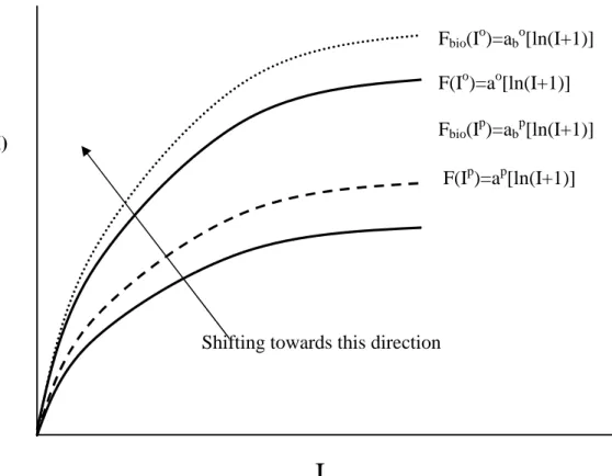
(6) Figures List. Figure 1.1 Framework of this dissertation ................................................................ 6 Figure 3.1 The relationship between production function and investment(homogeneous beliefs among investors) .............................18 Figure 3.2 The relationship between production function and investment(heterogeneous beliefs among investors) ............................21 Figure 3.3 The time line of event ............................................................................22 Figure 3.4 Thee nt r e p r e ne ur ’ sa l t e r na t i ve s ..............................................................23 Figure 3. 5Thee nt r e p r e ne ur ’ sp r i c i nga n dva l ua t i o nofd i ve r g e n ti nv e s t o r s (with unlimited wealth)...................................................................................24 Figure 3.6 Thee nt r e p r e ne ur ’ sp r i c i nga n dva l ua t i o nofd i ve r g e n ti nv e s t o r s (with limited wealth).......................................................................................27 Figure 4.1 The solution to the signaling equation...................................................31 Figure 4.2 The e vo l ut i o no faf i r m’ se a r ni n gss t r e a m(heterogeneous beliefs)........32 Figure 4.3 The relationship between earnings of a firm and cash dividend(homogeneous beliefs) ............................................................35 Figure 4.4 The relationship between earnings of a firm and cash dividend(heterogeneous beliefs) ...........................................................37 Figure. 4.5 The difference in cash dividend paid between MM and heterogeneous beliefs of investors.................................................................................38 Figure 4.6 The solution to heterogeneous beliefs ...................................................48 Figure 4.7 Shifted curve of a production function Fbio (I)=abi[ln(I+1)] as creating a new biotechnology ................................................................................51 Figure 4.8 The solution to heterogeneous beliefs as innovating a new medicine... 53. III.

(7) Chapter 1 Introduction 1.1 Motivation Dividend policy is one of the most important policies concerned with corporate finance for a firm, and it is a decision that balances the use of retained earnings be t we e nt hef i r m’ sr e i nve s t me nta ndt hepa y me ntt os ha r e hol de r s .I tde t e r mi ne s s ha r e h o l de r s ’c ur r e ntr e t ur na ndt hef i r m’ sf ut ur epr os pe c t ,a ndi ta l s oa f f e c t sbe ne f i t allocation between different groups of shareholders.. Therefore, dividend policy is an. important issue relating to the valuation of a firm. In many of the classic principle-agent relationships regarding dividend policy of a firm, asymmetric information is one of the most important frameworks such as the Miller and Rock (1985), and John and Williams (1985). to disagree.. However, they did not allow investors agree. On the basis of that there are heterogeneous beliefs existing among. divergent investors, the model constructed in this paper is not under asymmetric information but a heterogeneous framework.. I will determine and interpret optimal. di vi de ndpol i c yba s e donnotonl ybyma na ge r s ’ ,buta l s oi nve s t or s ’vi e wpoi nt s .. Classic literatures assume that investors have the same beliefs given the same information.. However, the common beliefs assumption is suitable for traditional and. matured industries because available information is rich and a large amount of experience has been accumulated.. Conversely, in this paper the common beliefs. assumption is not allowed even given the same information because people agree to disagree due to facing a completely new industry, i.e. biotechnology.. There have been some studies regarding diversity of opinions between different parties.. Manove and Padilla (1998) and DeMarzo et al. (1998) have ever considered. models where agents have different priors initially and updated in a Bayesian manner. However, in both cases agents are irrational in that they do not use all the information available to them in an optimal way.. In my analysis, all agents are fully rational.. 1.

(8) Allen and Gale (1999) argued that common priors assumption is appropriate when information is plentiful, a large amount of experience has been accumulated, and posterior beliefs have converged.. It can be argued that common priors. assumption is not appropriate when considering new industries such as biotechnology and new technologies such as personal computers.. They offered a model to compare. the effectiveness of financial markets and financial intermediaries in financing new industries and technologies in the presence of diversity of opinions.. The results. showed that financial markets tend to be superior when there is significant diversity of opinions.. However, it is complex and too many parameters were used to be practical.. In our model, heterogeneous beliefs of investors are directly given.. A simple, clear,. and general production/investment function is utilized to directly express real estimation on the future earnings of a firm. heterogeneity deeper.. This function will help to explore. More concrete results are therefore obtained.. The common priors assumption is not appropriate when considering new industries.. Harris and Raviv (1993) proposed a model allowing for differences in. prior beliefs.. Kandel and Pearson (1995) provided empirical evidence that trading. around earnings announcements is due to differences in priors.. However, their. models could not illustrate a concrete industry or a new technology.. In this paper, we. will take biotechnology as an example.. When a new medicine is innovated, there. will be heterogeneous beliefs on its future prospect given the same investment. Investors agree to disagree because the amount of data available based on actual experience with this new product is nonexistent or small.. Chen (2003) proposed a mathematical model to study dividend policy.. She. focused on how differences of opinions create incentives for the investors to trade. From the viewpoint of risk, she concluded that an optimistic investor perceives more risk and hence behaves like trend chasers.. Although she has ever found that high. dividend payout ratio mitigates the divergence in opinions among traders, how the optimal dividend policy is determined and changed according to heterogeneous beliefs is not yet discussed.. In this paper, not only does heterogeneous beliefs to result in. changing optimal dividend policy be studied but the degree of diversity of opinions be. 2.

(9) also considered.. Grullon et al. (2002) proposed maturity hypothesis to examine the relation between dividend changes and risk changes.. As firms mature, their investment. opportunities set shrinks, resulting in a decline in their future profitability.. The. decline in investment opportunities generates an increase in free cash flows, leading to an increase in dividends.. In our model, an increase or decrease in dividend is. according to the ratio of pessimistic to optimistic investors and heterogeneous beliefs of investors.. Bhattacharya (1979), Miller and Rock (1985), and John and Williams (1985) proposed that firms adjust dividends to signal their prospects.. A rise in dividend. typically signals that the firm will do better, and a decrease suggests that it will do worse.. In this research, however, dividend policy i snotde t e r mi ne dbyaf i r m’ s. c ha r a c t e rbuti nve s t or s ’vi e wpoi nt s . Ast hebe l i e f sofi nve s t or si nc l udi ng bot h opt i mi s t i ca ndpe s s i mi s t i cone sc ha ng e ,af i r m’ sopt i ma ldi vi de ndpol i c ywi l lbehe nc e adjusted.. Low dividend policy is appropriate as in invest or s ’ be l i e f sa r e. simultaneously increased.. We interpret this novel result not based on the traditional. signaling theories, but on heterogeneity.. Specifically, the ratio of pessimistic to. optimistic investors and the degree of divergent beliefs could change the optimal dividend policy.. This research may provide a useful reference for researchers attempting to develop a theoretical model regarding optimal dividend policy under a framework classified by heterogeneous beliefs of investors.. In addition, dividend policy in a. new industry such as biotechnology will be also illustrated to enrich this study.. 3.

(10) 1.2 Research objectives This paper is to derive a model regarding optimal dividend policy with heterogeneous beliefs of divergent investors.. Different from typical framework. based on information asymmetry, this paper is under full information. heterogeneous. beliefs. by divergent. investors. is. introduced. to. Concept of form. the. pr oduc t i on/ i nve s t me ntf unc t i on a nd f ur t he r mor ei nf l ue nc eaf i r m’ sva l ue ,he nc e changing dividend policy.. This paper is to derive a model regarding optimal. dividend policy with heterogeneous beliefs of divergent investors.. To summarize, the purpose of this paper is to derive the optimal dividend policy with heterogeneous beliefs of divergent investors.. Framework and concept of. heterogeneous beliefs among divergent investors are introduced.. Heterogeneous. beliefs on future earnings of a firm is emphasized and formulated in this research.. 4.

(11) 1.3 Dissertation framework This dissertation is segmented into five chapters with each one synopsized below: Literature review is introduced in Chapter 2.. Dividend policy with heterogeneous. beliefs - the full information model is formulated in Chapter 3.. Dividend policy with. heterogeneous beliefs - the asymmetric information model is given in Chapter 4. Conclusions and suggestions are arranged in Chapter 5.. 5.

(12) Motivation and objectives. Literature review. Dividend policy-one period, full information model. Homogeneous beliefs among the investors. Dividend policy-two period, asymmetric information model. Heterogeneous beliefs among the investors. Optimistic investors with limited wealth. Homogeneous beliefs among the investors. Optimistic investors with unlimited wealth. Conclusion and suggestion. Figure 1.1 Framework of this dissertation. 6. Heterogeneous beliefs among the investors. Comparative static analysis.

(13) Chapter 2. Literature review. 2.1 Dividend policy There have been many theoretical studies on dividend policy.. Miller and. Modigliani (1961) had a seminal contribution to research on dividend policy.. Prior. to this, most researchers believed that the more dividends a firm paid, the more valuable the firm would be.. This view was derived from an extension of the. discounted dividends approach to firm valuation, which says that the value V0 of the firm at date 0, if the first dividends are paid one period from now at date 1, is given by  D the formula V0=  t t , where Dt is the divided paid by the firm at the end of t 1 (1 rt ). period t, and rt i st hei nve s t or s ’oppor t uni t yc os tofc a pi t a lf orpe r i odt . Gor do n( 1 9 5 9 ) a r g ue dt ha ti nve s t or s ’r e qui r e dr a t eofr e t ur nr t would increase with retaining of earnings and increased investment.. Although the future dividend stream would. presumably be larger as a result of the increase in investment (i.e., Dt would grows faster), Gordon felt that higher rt would overshadow this effect.. The reason for the. increase in rt would be the greater uncertainty associated with the increased investment relative to the safety of the dividend.. Miller and Modigliani pointed out that this view of dividend policy incomplete and they developed a rigorous framework for analyzing payout policy.. They showed. t ha twha tr e a l l yc ount si st hef i r m’ si nve s t me ntpo l i c y . Asl onga si nve s t me ntpol i c y doe s n’ tc ha nge ,a l t e r i ngt hemi xofr e t a i ne de a r ni ng sa ndpa y outwi l lnota f f e c tt he f i r m’ sva l ue . Thef r a me wor kh a sf or me dt hef ounda t i onofs ubs e que ntwork on dividends and payout policy in general.. It is important to note that their framework. is rich enough to encompass both dividends and repurchases, as the only determinant ofaf i r m’ sva l uei si t si nve s t me ntpol i c y .. The dividend literature that followed the Miller and Modigliani article attempted to reconcile the indisputable logic of their dividend irrelevance theorem with the. 7.

(14) notion that both managers and markets care about payouts, and dividends in particular. The theoretical work on this issue suggests five possible imperfections that management should consider when it determines dividend policy.. They are taxes,. asymmetric information, an incomplete contract, institutional constraints and transaction costs.. First, if dividends are taxed more heavily than capital gains, and investors cannot use dynamic trading strategies to avoid this higher taxation, then minimizing dividends is optimal.. Second, if managers know more about the true worth of their. firm, dividends can be used to convey the information to the market, despite the costs associated with paying those dividends.. Third, if contracts are incomplete or are not. fully enforceable, equityholders may use dividends to discipline managers or to expropriate wealth from debtholders.. Fourth, if various institutions avoid investing. in non-or-low-dividend-paying stocks because of legal restrictions, management may find that it is optimal to pay dividends despite the tax burden it imposes on individual investors.. Fifth, if dividends payments minimize transaction costs to shareholders,. then positive dividend payout may be optimal.. The best known literature of asymmetric information are those of Bhattacharya (1979), Miller and Rock (1985), and John and Williams (1985).. The basic idea in all. these models is that the firms adjust dividends to signal their prospects.. A rise in. dividend typically signals that the firm will do better, and a decrease suggests that it will do worse.. These theories may explain why firms pay out so much of their. earnings as dividends.. Bhattacharya has the feature that dividends and repurchase. are perfect substitutes for one another.. It does not matter whether the good firm. signals its value through repurchasing shares or paying dividends, because the end result will be the same.. Therefore, one of the implications of these models is that. dividends and repurchases are perfect substitutes.. Miller and Rock (1985) also constructed a two-period model.. In their model, at. time zero firms invest in a project, the profitability of which cannot be observed by investors.. At time 1, the project produces earnings and the firm uses these to finance. 8.

(15) its dividend payment and its new investment. earnings or the new investment.. Investors cannot observe either. An important assumption in their model is that. some shareholders want to sell their holdings in the firm at time 1, and that this factor e nt e rma na g e r ’ si nve s t me nta ndpa y outde c i s i ons . Att i me2,t hef i r m’ si nve s t me nt again produces earnings.. A critical assumption of the model ist ha tt hef i r m’ s. earnings are correlated through time.. This setting implies that the firm has an. incentive to make shareholders believe that the earnings at time 1 are high so that the shareholders who sell will receive a high price.. Since both earnings and investment. are unobservable, a bad firm can pretend to have high earnings by cutting its investment and paying out high dividends.. A good firm must pay a level of. dividends that is sufficiently high to make it unattractive for bad firms to reduce their investment enough to achieve the same level. number of attractive features.. The Miller and Rock theory has a. The basic story that firms shave investment to make. dividends higher and signal high earnings is entirely plausible.. Unlike the. Bhattacharya model, the Miller and Rock theory does not rely on assumptions that are difficult to interpret, such as firms being able to commit to a dividend level. J ohna ndWi l l i a m’ ss t a r t i ngpoi nti st hea s s umpt i ont ha ts ha r e hol de r si naf i r m have liquidity needs tha tt he ymus tme e tbys e l l i ngs omeoft he i rs ha r e s . Thef i r m’ s managers act in the interest of the original shareholders and know the true value of the firm.. Outside investors do not.. If the firm is undervalued when the shareholders. must meet their liquidity needs, then these shareholders would be selling at a price below the true value.. However, suppose the firm pays a dividend, which is taxed.. If outside investors take this as a good signal, then the share price will rise. Shareholders will have to sell less equity to meet their liquidity needs and will ma i nt a i nahi g he rpr opor t i ona t es ha r ei nt hef i r m. J ohna ndWi l l i a m’ smode la voi d the objection to most signaling theories of dividends.. Firms do not repurchase shares. to avoid taxes, because it is precisely the cost of the taxes that makes dividends desirable.. This is clearly an important innovation.. After the Miller and Rock (1985) and John and Williams (1985) papers, a number of other theories with multiple signals were developed.. 9. Ambarish, John, and.

(16) Williams (1987) constructed a single-period model with dividends, investment, and stock repurchases.. Williams (1988) developed a multi-period model with these. elements and showed that in the efficient signaling equilibrium, firm typically pay dividends, choose their investments in risky assets to maximize net present value, and issue new stock.. Constantinides and Grundy (1989) focused on the interaction. between investment decisions and shares repurchase and financing decisions in a signaling equilibrium.. Brenheim (1991) also provided a theory of dividend in which signaling occurs because dividends are taxed more heavily than repurchases.. In this model, the firm. controls the amount paid by varying the proportion of the total payout that is in the form of dividends, rather than repurchases. amount of taxes to provide the signal.. A good firm can choose the optimal. As with the John and Williams model,. Br e nhe i m’ smode ldoe snotpr ovi deag oode xpl a na t i onofdi vi de nds moot hi ng .. Allen, Bernardo, and Welch (2000) took a different approach to dividend signaling. As in the previous models, dividends are a signal of good news.. However, in their. model firms pay dividends because they are interested in attracting a better-informed clientele.. Untaxed institutions are the primary holders of dividend-paying stocks. because they are a tax-disadvantaged payout method for other potential stockholders. Another reason why good firms like institutions to hold their stock is that these stockholders are better informed and have a relative advantage in detecting high quality firm.. Low-quality firms do not have the incentive to mimic, since they do. not wish their true worth to be revealed.. Paying dividends increases the chance that. institutions will detect the f i r m’ squa l i t y . Kumar (1988) provided a theory of dividend smoothing.. In his model, the. managers who make the investment decision know the true productivity type of the firm but the outside investors do not.. Managers will try to achieve lower investment. by unde r r e por t i ng t hef i r m’ spr oduc t i vi t yt y pe . Gr ul l on e ta l .( 2002 )pr opos e d maturity hypothesis to say about the relation between dividend changes and risk changes.. They proposed that there are several elements that contribute to firms. becoming mature.. Thus, a dividend increase indicates that a firm has matured.. 10.

(17) 2.2 Heterogeneous beliefs Heterogeneous beliefs on a firm’ s prospects, i.e., on the distribution of the firm’ s future cash flows, may stem from asymmetric information.. However, Bigus (2003). argued such beliefs are possible even in the case of symmetric information. When they share the same information, people have heterogeneous beliefs just because they evaluate the same information differently.. First of all, there is empirical evidence. that human beings may not use all the information available to them and instead select data that is available to their consciousness. to their judgments.. Second, people tend to stick too closely. Third, people make mistakes when they calculate with. probabilities and, thus, may end up with different density functions on future returns. Fourth, even if we discount “ bounded rationality”issues, we find that people may evaluate (new) information differently when they have different “ message services” , for instance, when they have different experiences or when they use differing theories and ideas.. Fifth, in situations of uncertainty with no concrete probabilities, to derive. a density function on future returns people are often required to transform the information available into probabilities. They may consider some level of uncertainty differently, depending on how much they dislike uncertainty.. Garmaise (2001) proposed when people share the same information, they could have heterogeneous beliefs just because they evaluate the information differently. Wang (1998) developed a multi-period trading model in which traders face both asymmetric information and heterogeneous prior beliefs. Heterogeneity arises because traders agree to disagree on the precision of an informed trader’ s private signal. In equilibrium, the informed trader smooths out her trading on asymmetric information gradually over time, but concentrates her entire trading on heterogeneous beliefs toward the last few periods.. There is a long tradition in economics of allowing for differences in prior beliefs. For example, the Arrow-Debrew-Mackenzie (ADM) model and the fundamental theorems of welfare economics allow for different priors.. The well-known model of. stock market resource allocation developed by Diamond (1967) has this feature.. 11. A.

(18) number of important finance papers such as Linter (1965) and Ross (1976) have also allowed for differences in prior beliefs.. Kandel and Pearson (1995) provide. empirical evidence that trading around earnings announcements is due to differences in priors.. The common prior assumption is appropriate when information is plentiful, a large amount of experience has been accumulated. This is the type of situation to which standard finance models apply.. However, it can be argued that the common. prior assumption is not appropriate since the amount of data available based on actual experience with new products or technologies are nonexistent or small (Allen and Gale, 1999).. When considering new industries such as biotechnology, differences in. views would appear.. Causal empiricism suggests that there is a wide variation in. view on the effectiveness and value of an innovation immediately after the innovation has occurred.. In this study, there is diversity of opinion and people agree to disagree.. 12.

(19) 2.3 Dividend policy with heterogeneous beliefs among the investors In many of the classic principle-agent relationships regarding dividend policy of a firm, asymmetric information is one of the most important frameworks such as the Miller and Rock (1985), and John and Williams (1985). investors agree to disagree.. However, they did not allow. On the basis of that there are heterogeneous beliefs. existing among divergent investors, the model constructed in this paper is not under asymmetric information but a heterogeneous framework.. I determine and interpret. opt i ma ldi vi de nd pol i c y ba s e d on notonl y by ma na g e r s ’ ,buta l s oi nve s t or s ’ viewpoints.. Classic literatures assume that investors have the same beliefs given the same information.. However, the common beliefs assumption is suitable for traditional and. matured industries because available information is rich and a large amount of experience has been accumulated.. Conversely, in this study the common beliefs. assumption is not allowed even given the same information because people agree to disagree due to facing a completely new industry, i.e. biotechnology.. There have been some studies regarding diversity of opinions between different parties.. Manove and Padilla (1998) and DeMarzo et al. (1998) have ever considered. models where agents have different priors initially and updated in a Bayesian manner. However, in both cases agents are irrational in that they do not use all the information available to them in an optimal way.. In our analysis, all agents are fully rational.. Allen and Gale (1999) argued that common priors assumption is appropriate when information is plentiful, a large amount of experience has been accumulated, and posterior beliefs have converged.. It can be argued that common priors. assumption is not appropriate when considering new industries such as biotechnology and new technologies such as personal computers.. They offered a model to compare. the effectiveness of financial markets and financial intermediaries in financing new industries and technologies in the presence of diversity of opinions.. The results. showed that financial markets tend to be superior when there is significant diversity of. 13.

(20) opinions.. However, it is complex and too many parameters were used to be practical.. In our model, heterogeneous beliefs of investors are directly given.. A simple, clear,. and general production/investment function is utilized to directly express real estimation on the future earnings of a firm. heterogeneity deeper.. This function helps us to explore. More concrete results are therefore obtained.. The common prior assumption is not appropriate when considering new industries.. Harris and Raviv (1993) proposed a model allowing for differences in. prior beliefs.. Kandel and Pearson (1995) provided empirical evidence that trading. around earnings announcements is due to differences in priors.. However, their. models could not illustrate a concrete industry or a new technology.. In this paper, we. will take biotechnology as an example.. When a new medicine is innovated, there. will be diversity of opinions on its future prospect given the same investment. Investors agree to disagree because the amount of data available based on actual experience with this new product is nonexistent or small.. Chen (2003) proposed a mathematical model to study dividend policy.. She. focused on how differences of opinions create incentives for the investors to trade. From the viewpoint of risk, she concluded that an optimistic investor perceives more risk and hence behaves like trend chasers.. Although she has ever found that high. dividend payout ratio mitigates the divergence in opinions among traders, how the optimal dividend policy is determined and changed according to heterogeneous beliefs is not yet discussed.. In this paper, not only does heterogeneous beliefs to result in. changing optimal dividend policy be studied but the degree of diversity of opinions be also considered.. Grullon et al. (2002) proposed maturity hypothesis to examine the relation between dividend changes and risk changes.. As firms mature, their investment. opportunities set shrinks, resulting in a decline in their future profitability.. The. decline in investment opportunities generates an increase in free cash flows, leading to an increase in dividends.. In our model, an increase or decrease in dividend is. according to the ratio of pessimistic to optimistic investors and heterogeneous beliefs. 14.

(21) of investors.. Bhattacharya (1979), Miller and Rock (1985), and John and Williams (1985) proposed that firms adjust dividends to signal their prospects.. A rise in dividend. typically signals that the firm will do better, and a decrease suggests that it will do worse.. In this study, however, dividend policy is not determine d by af i r m’ s. c ha r a c t e r i s t i cbuti nve s t or s ’vi e wpoi nt s . Ast hebe l i e f sofi nve s t or si nc l udi ngbot h opt i mi s t i ca ndpe s s i mi s t i cone sc ha ng e ,af i r m’ sopt i ma ldi vi de ndpol i c ywi l lbehe nc e a dj us t e d. Low di vi de nd pol i c yi sa ppr opr i a t ea si ni nve s t or s ’ be l i e fs are simultaneously increased.. We interpret this result not based on the traditional. signaling theories, but on heterogeneity.. Different from the typical theoretical work regarding dividend policy of a firm, we will focus on studying the effect of investors with heterogeneous beliefs on changing investment/dividend policy. introduced.. The concept of agreeing to disagree will be. Differences in views would appear to be due to differences in priors.. There is diversity of opinions on a firm’ s future prospect.. The framework of the. model under the conventional framework-homogeneous beliefs among investors and another framework - heterogeneous beliefs among investors will be compared.. Then, we will explore the optimal dividend policy of a firm with heterogeneous beliefs-the asymmetric information model. We will first review the Miller and Rock (1985) model regarding dividend policy under asymmetric information.. Next, we. will propose a two-period model to conduct dividend policy with heterogeneous beliefs among the investors.. Last, heterogeneous beliefs on future earnings of a firm. is emphasized and formulated in our model.. Specifically, the ratio of pessimistic to. optimistic investors and the degree of divergent beliefs may change the optimal dividend policy will be studied.. 15.

(22) Chapter 3. Investment/dividend policy with heterogeneous beliefs-the full information model. This chapter explores the investment/dividend policy of a firm with heterogeneous beliefs among investor.. Different from the typical theoretical work. regarding dividend policy of a firm, I focus on studying the effect of investors with heterogeneous beliefs on changing investment/dividend policy. sections included in this chapter.. There are three. Section 3.1 describes the framework of the model. under the conventional framework-homogeneous beliefs among investors.. Section. 3.2 introduces another framework - heterogeneous beliefs among investors. Differences in views would appear to be due to differences in priors. diversity of opinions on a firm’ s future prospect.. There is. Section 3.3 is the modeling of. heterogeneous beliefs among investors and how to affect a firm’ s investment/dividend policy.. 16.

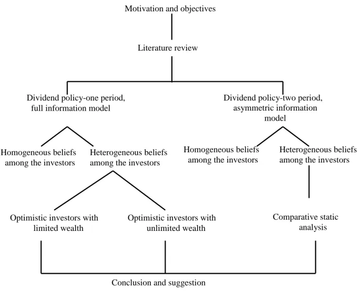
(23) 3.1 Homogeneous beliefs among the investors The common prior assumption is appropriate when information is rich and a large amount of experience has been accumulated. which standard finance models apply.. This is the type of situation to. It is appropriate to the traditional industries. since the amount of data available with old products or technologies is rich.. 3.1.1 Homogeneous beliefs In typical finance model, it is assumed that investors have common information, and hence the same prior probability beliefs. homogeneous beliefs.. Investors are assumed to have. Given a set of common information, all investors agree that. firm’ s future earnings are the same.. This means that all investors will agree about. an asset’ s expected cash flows.. 3.1.2 Homogeneous beliefs in the production/investment function The production/investment function F(I) is assumed to have the following  properties: F C ∞ ; F(I)≧0; F ＞0; and F  ＜0.. The production function is. described by the following equation: F(I)=a[ln(I+1)]; a>0. (3.1). where I is the investment; a is a constant and the same estimated by all of the investors.. That is, beliefs on earnings among investors are homogeneous.. The. first-order partial derivate of Equation (3.1) is F (I ) =. a I 1. (3.2). where F  (I ) is strictly increasing in I and must be larger than zero because a and I are larger than zero according to the assumption.. This means that the slope of. production/investment function F(I) against investment I is strictly positive.. The. second-order partial derivate of F(I) is derived by  F (I ) =-. a ( I 1) 2. (3.3). 17.

(24)  where F  (I ) is strictly decreasing in I and must be negative because a and I are. positive.. This means that the production/investment function F(I) is a concave. function.. The relationship between production F(I) and investment I is depicted in. Figure 3.1.. Slope=. a I 1. F(I)= a[ln(I+1)]. F(I). I Figure 3.1 The relationship between production function and investment (homogeneous beliefs among investors). As shown in Figure 3.1, the production function F(I) increases as the investment I increases.. F(0) is assumed to be zero and the slope,. because a and I are positive.. a , is strictly positive I 1.  The second-order partial derivate, F  (I ) =-. a , ( I 1) 2. derived from Equation (3.3) is always negative because both a and I are positive.. It. indicates that the production function concaves in investment, that is, the slope decreases as the investment increases.. 18.

(25) 3.2 Heterogeneous beliefs among the investors 3.2.1 Heterogeneous beliefs The common priors assumption is appropriate when information is rich and a large amount of experience has been accumulated. which stand finance models apply.. This is the type of situation to. However, it is not appropriate when considering. new industries such as biotechnology.. Since the amount of data available with new. products or technologies is nonexistent or small, such differences in view would appear to be due to differences in priors.. In this study, there is diversity of opinions. and people agree to disagree.. Relaxing the preceding assumption, investors have common information but agree to disagree about the future earnings of a firm.. Divergent investors receive. common information, but differ in the way in which they interpret this information. We assume that there are two types of investors including the optimistic and pessimistic ones.. Each type of investor’ s information is independent of the other. type of investors, and of the common information.. Investors have heterogeneous beliefs in the future earning of a firm since they have different prior beliefs, will interpret information differently.. That is, they have. common information but agree to disagree about the future earnings. conditions to constitute such heterogeneity.. There are three. People who respect each other’ s. opinions and nevertheless disagree about subject probabilities is the first possibility. Second, heterogeneity of beliefs does not come from asymmetric information but rather from intrinsic differences in how to view the world.. People agree to disagree,. which implies that the investors do not generate Bayesian updating of individual beliefs.. Third, as Harris and Raviv (1993) argued, investors share common prior. beliefs and receive common information but differ in the way in which they interpret this information.. Some investors will become pessimistic, others will interpret the. same information as grounds for optimism.. There are two groups of investors called. optimists and pessimists, agreeing to disagree about the parameter a.. 19.

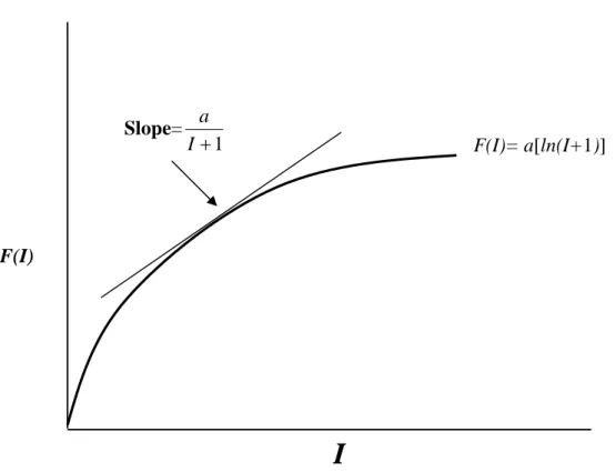
(26) 3.2.2 Heterogeneous beliefs on Production/investment function The production/investment function is not the same as that of Equation (3.1).. It. is described by the following equation: F(I)=ai[ln(I+1)]; i o,p. (3.4). where ai is not a constant the same as that of homogeneous case. future earnings among investors are heterogeneous.. The beliefs on the. The first-order partial derivate. of (3.4) is given by F (I ) =. ai >0 I 1. (3.5). where F  (I ) is strictly increasing in I and must be larger than zero because both ai and I are positive according to the assumption.. This means that the slope of. production function F(I) against investment I is strictly positive.. The second-order. partial derivate of Equation (3.4) is derived by  F (I ) =-. ai <0 ( I 1) 2. (3.6).  where F  (I ) is strictly decreasing in I and must be smaller than zero because both ai. and I are positive. concave function.. This means that the production/investment function F(I) is a The relationship between F(I) and I is depicted in Figure 3.2.. As shown in Figure 3.2, there are three curves of production functions including the optimistic and pessimistic investors plus the homogeneous case respectively. Viewed by the optimistic investors, production function, F(Io)=aoln(I+1), is always largest at each point.. Conversely, production function viewed by pessimistic investors,. F(Io) =aoln(I+1), is always smallest.. Production function F(I) viewed by all of the. investors increases as the investment I increases. positive because both ai and I are positive.  F (I ) =-. The slope,. ai , I 1. is strictly. The second-order partial derivate,. ai , derived from Equation (3.6) is always negative. ( I 1) 2. It indicates that. production/investment function concaves in investment, that is, the slope decreases as investment increases.. 20.

(27) F(I)=aln(I+1). F(Io) F(I). Slope=. ao I 1. Slope=. a I 1. Slope=. F(Io)=aoln(I+1). F(Ip)=apln(I+1). ap I 1. F(I) F(Ip). I. Figure 3.2 The relationship between production function and investment (heterogeneous beliefs among investors). 21.

(28) 3.3 Description of the model We consider an economy that there are no transaction costs or taxes.. A firm is. initially owned by an entrepreneur, who wants to find the value-maximizing investment expenditure I and cash dividend D before selling his shares to public investors and leaving the market.. At T=0, the firm is endowed with cash earnings. X0>0 and production function F(I)=ai[ln(I+1)].. There are two groups of investors. called optimists and pessimists, agreeing to disagree about the parameter ai.. The. optimists believe that ai =ao and the pessimists believe that ai =ap, where ao > ap≧1. The total wealth of the optimists is W>0.. Figure 3.3 shows the time line of event.. A firm endowed with cash earnings. F(I)=ai[ln(I+1)]. X0. Entrepreneur sells his. Entrepreneur prices the stock, invests. shares to the investors. I and decides cash dividend.. and leaves the market.. T=0. T=1. Figure 3.3 The time line of event. As shown in Figure 3.3, the entrepreneur decides dividend policy D and invests I in a production process.. 3.3.1 The entrepreneur’ s decision problem For the entrepreneur, there are two important decisions when he wants to ma xi mi z et hef i r m’ sva l ue . The first decision is pricing the stock at some value, the other one is determining the dividend/investment.. Divergent types of investors with. heterogeneous beliefs will affect the decisions, and thus result in changing the dividend/investment policy.. 22.

(29) Investors with unlimited wealth sell only to the optimistic investors Entrepreneur. Investors with limited wealth. sell to both the optimistic and pessimistic investors. Figure 3.4 The entrepreneur’ s alternatives. Figure 3.4 shows the entrepreneur’ s decision alternatives.. The entrepreneur has. two alternatives: he can sell the shares only to the optimistic investors, or he can sell some shares to the pessimists upon seeing the valuation by different types of investors and the wealth of the optimists.. If the type-o investors have no wealth limit, the. entrepreneur will implement the first alternative-selling only to the optimists. Conversely, the entrepreneur will choose to implement the second alternative-selling to both the optimists and pessimists.. The key point is divergent types of investors.. 3.3.2 With unlimited wealth for the optimistic investors Due to with unlimited wealth limit, the entrepreneur will implement the first alternative-selling the stock only to the optimistic investors.. If the entrepreneur. chooses to sell all the shares only to the type-o investors, under linear pricing he will price the stock at P= X0-I+ao[ln(I+1)]. (3.7). The price is the same as the valuation of type-o investors so as that there is no incentive to attractive type-p investors to buy any share because the price is much higher than that of the valuation they estimate.. Hence, all the shares are to be sold to. the optimistic investors. The entrepreneur gains the most profit. Definition 3.1 Cash dividend paid by a firm is defined as high dividend if D> X0-a+1;. 23.

(30) as low dividend if D< X0-a+1. Proposition 3.1 A low dividend policy is appropriate with cash dividend D= X0-ao+1 as the shares are sold only to the type-o investors. Proof. The optimists’valuations for the firm are described as Vo= X0-I+ao[ln(I+1)]. (3.8). The pessimists’valuations for the firm are Vp= X0-I+ap[ln(I+1)]. (3.9). The entrepreneur maximizes his profit by pricing the stock at the highest valuation estimated by different types of investors.. Due to without limited endowment for the. optimistic investors, all the shares will be sold to the optimistic investors.. The price. of the stock is P= X0-I+ao[ln(I+1)]. Entrepreneur’ s pricing:. (3.10). Valuation of Type-o investors:. o. Vo=X0-I+ao[ln(I+1)]. P=X0-I+a [ln(I+1)]. Valuation of Type-p investors: Vp=X0-I+ap [ln(I+1)]. Figure 3.5 The entrepreneur’ s pricing and valuation of divergent investors (with unlimited endowment). As shown in Figure 3.5, the price is the same as the valuation of type-o investors.. There is no incentive to attract type-p investors to buy any shares because. the price is higher than that of the valuation they estimate. endowment limit assumption for the optimistic investors.. Also, there is no Therefore, all the shares. are to be sold to type-o investors.. To find the optimal investment expenditure and dividend policy, we take the first-order partial differentiation to Equation (3.10).. 24. The first-order condition of.

(31) (3.10) requires  P =0  I. =-1+. ao I 1. (3.11). Equating the preceding equation, we have the optimal investment expenditure I*= ao-1. (3.12). Substituting Equation (3.12) into (3.10), we get the equilibrium price P*=X0- ao+1+aoln(ao). (3.13). Optimal dividend policy is then derived D*= X0- I* = X0- ao+1. (3.14). Because ao is larger than a and ap according to the previous assumption, therefore D*= X0- ao+1 < X0- a+1 <X0- aP+1. (3.15). According to Equation (3.15) and Definition 3.1, we can conclude that a low dividend policy is appropriate with cash dividend D= X0- ao+1 is optimal as the shares are sold only to type-o investors.. The entrepreneur will fail to issue the stock to the market if he still prices the stock at the same as implementing alternative 1 when the wealth of optimists is less than X0-ao+1+aoln(ao).. If the entrepreneur still prices the stock at P=X0-I+aoln(I+1). which is the same as implementing alternative 1.. Based on (3.12), (3.13) and (3.14),. in equilibrium the optimal investment expenditure will be I*= ao-1 And pricing the stock at P=X0-ao+1+aoln(ao) If the wealth of the optimists is less than this value, they will not have enough money to buy the shares.. That is, if W<P(=X0-ao +1+ ao ln(ao)). 25.

(32) As a consequence, the entrepreneur will fail to issue the stock pricing at P=X0-ao+1+aoln(ao) because there is not any investor willing to buy. 3.3.3 With limited wealth for the optimistic investors In order to focus on exploring the effect of heterogeneous beliefs on changing the optimal dividend policy of a firm, a stronger assumption must be made to make sure at least one pessimistic investor gets to hold some share.. We assume the wealth of. optimistic investors W is limited so as that they have not enough money to buy all the shares, and at least one pessimistic investor will buy some shares.. The entrepreneur. must consider selling the shares to both optimistic and pessimistic investors.. If the. entrepreneur still prices the stock at P=X0-I+aoln[(I+1)] which is the same as implementing alternative 1, there will be not any one to buy the stock because the optimistic investors have not enough money due to wealth constraint.. The following. proposition is to derive another investment/dividend policy as the wealth of optimistic investors is limited. Proposition 3.2 A high dividend policy is appropriate with limited wealth for the optimistic investors as the stock are sold not only to type-o investors, but also to at least one type-p investor. Proof. The entrepreneur wants to maximize his profit by pricing the stock at the highest valuation estimated by different types of investors.. If the entrepreneur still. prices the stock at P=X0-I+aoln[(I+1)] the same as that of proposition 3.1, there will be not anyone to buy the stock. strategy.. Therefore, the entrepreneur has to change the. Implementing alternative 2 as shown in Figure 3.6, the entrepreneur will. price the stock at P=X0-I+apln(I +1). (3.16). Assume that the wealth of the optimistic investors W is less than the valuation for the firm by them.. That is, W<X0+1- aP+apln(aP). 26. (3.17).

(33) Valuation of Type-o investors: Vo=X-I+aoln(I+1). Valuation of Type-p investors:. Entrepreneur’ s pricing:. Vp=X-I+apln(I+1). P= X-I+apln(I+1). Figure 3.6 Thee nt r e pr e ne ur ’ spr i c i nga ndva l ua t i onofdi ve r g e nti nve s t or s (with limited wealth). As shown in Figure 3.6, the pricing is the same as the valuation of type-p investors. In equilibrium, both type-o and –p investors will hold some shares. The first-order condition of Equation (3.16) requires  P =0  I. =-1+. ap I 1. (3.18). Equating the preceding equation, we have the optimal investment expenditure I*= ap-1. (3.19). Substituting (3.19) into (3.16), we get the equilibrium price P*=X0-ap+1+apln(ap). (3.20). Optimal dividend policy is then derived D*= X0- I* = X0- ap +1. (3.21). Based on the previous assumption, ap <a< ao. (3.22). We can derive D*= X0- ap+1 > X0- a+1. 27.

(34) > X0- ao +1. (3.23). Consequently, a high dividend policy is appropriate as the stocks are sold not only to type-o, but also at least one type-p investor holding some shares.. 28.

(35) Chapter 4. Dividend policy with heterogeneous. beliefs-the asymmetric information model Chapter 3 describes optimal dividend policy with heterogeneous beliefs of investors when an entrepreneur wants to maximize a firm’ s value.. Different from. Chapter 3, this chapter explores the optimal dividend policy of a firm with heterogeneous beliefs-the asymmetric information model.. I focus on studying the. effect of divergent types of investors on changing the optimal dividend policy. are four sections included in this chapter.. Section 4.1 reviews the Miller and Rock. (1985) model regarding dividend policy under asymmetric information. is the description of the model.. There. Section 4.2. In section 4.2, I propose a two-period model to. conduct dividend policy with heterogeneous beliefs among the investors. is the entrepreneur’ s decision problem. analysis.. 29. Section 4.3. Section 4.4 is the comparative static.

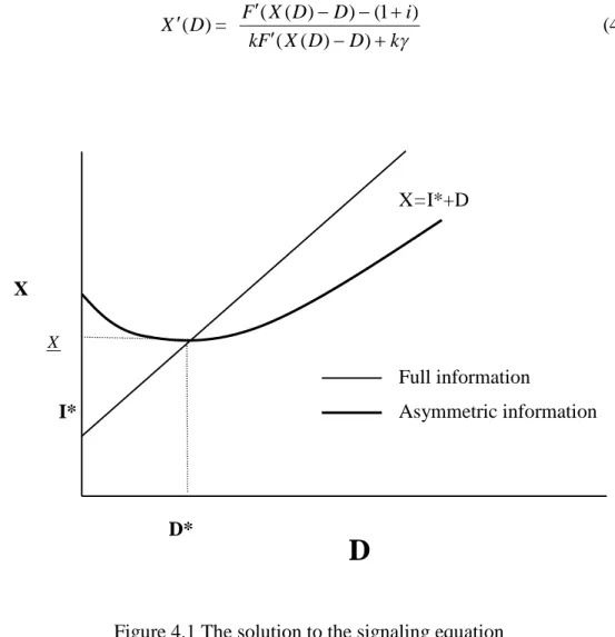
(36) 4.1 The Miller and Rock model Miller and Rock (1985) proposed a model to study dividend policy under asymmetric information.. In their model, managers have more information of a firm. than outside investors regarding the true state of the firm’ s current earnings.. They. show that a consistent signaling equilibrium exists under asymmetric information and the trading of shares that restores the time consistency of investment policy, but leads in general to lower levels of investment than the optimum achievable under full information.. More dividend paid is to signal a good firm.. Asymmetry of information in the Miller and Rock model means differences in information about earnings lead in differences in the perceived value of the firm. Viewed by the managers and directors (insider), the value of a firm is described as V1d =D1+. 1 ~] [F(I1)+γ  1 1 i. (4.1). For the market outsider, the value of the firm is given by V1m =D1+. 1 ~ ｜φm] [ E1m F(I1)+γ  1 1 i. (4.2). One objective function for the firm compatible with that requirement is a function in which the firm’ s managers attach weights to the interest of each group proportional to the values of their holdings.. The manager’ s problem can then be written as. m d Max W1=k V1 +(1-k) V1 D1 ,I1. = k { D1+. 1 ~ ｜φm]} [ E1m F(I1)+γ  1 1 i. +(1-k) {D1+. 1 ~ ]} [F(I1)+γ  1 1 i. (4.3). Subject to D1+I1=X1 where k is the fraction of the shares owned by the selling stockholders.. The. first-order condition for a maximum of (4.3) with respect to D1 for given X1 requires  V1  Vp +(1-k) =0  D  D m. k. 30. (4.4).

(37) The solution is described as X (D ) =. F ( X ( D) D) (1 i ) kF  ( X ( D) D) k. (4.5). X=I*+D. X X. Full information Asymmetric information. I*. D*. D. Figure 4.1 The solution to the signaling equation (Miller and Rock, 1985 Journal of Finance p.1044). Figure 4.1 shows the solution of Equation (4.5). if X  (D ) is positive.. A maximum occurs if and only. That is, the firm always chooses a dividend lying along the. increasing portion of X(D).. Thus, only dividend exceed D* are optimal.. The larger. a firm’ s earnings, the larger its dividend, beginning with lowest firm which pays D*. X(D) is an increasing function over the domain of observed dividends.. Based on. Equation (4.5), X(D)-D must be less than the Fisherian optimum level of investment.. 31.

(38) 4.2 Description of the model Following the Miller and Rock (1985) model, a two-period model is assumed that there are no transaction costs or taxes.. The stock is issued by an entrepreneur at. T=0 to the public investors, and the manager can commit to any dividend policy. ~ The evolution of firm’ s earnings stream, X t , is described by the following equations: ~ ~ X 1 =F(I0)+  1. (4.6). ~ ~ X 2 =F(I1)+  2 ~ ~ = F( X 1 -D1)+  2. (4.7). At T=0 (the past), the firm invested I0 in a production process whose output at the end of the period is F(I0) plus a random increment. the firm’ s earnings.. The sum of the two constitutes. At the start of period 1 (the present), those earnings are dividend. payment D1 and invest I1.. The investment I1 yields an end-of-period output of F(I1) ~ plus another random increment. The total earnings, X 2 , are distributed to the stock holders at the start of period 2 (the future) and the firm is disbanded.. Firm invested I0. T=0. Fi r m’ se a r ni ng s ~ ~ X 1 =F(Io)+  1 Type-O and Type-P receive common information but interpret differently Firm invests I1 Pays D1. T=1. Fi r m’ searnings ~ ~ X 2 =F(I1)+  2. T=2. Figure 4.2 The evolution of a firm’ s earnings stream (heterogeneous beliefs). 32.

(39) Figure 4.2 shows the evolution of a firm’ s earnings stream.. Different from the. Miller and Rock (1985) theory, there are two types of investors including the optimistic and pessimistic involved in this model.. The investors are assumed to be. risk averse and short-sale constraints to ensure stock trading equilibrium as Allen and Gale (1994) and Harris and Raviv (1993) argued. irrational and does not know the true earnings.. 33. The manager is assumed to be.

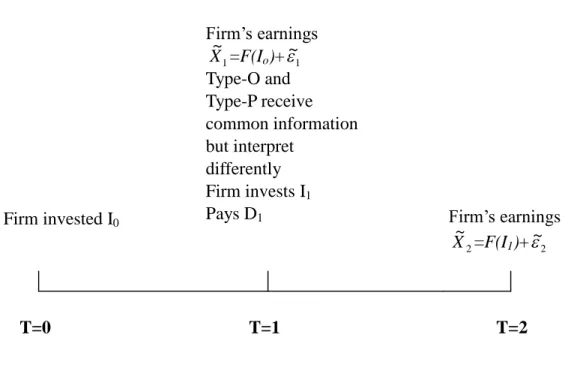
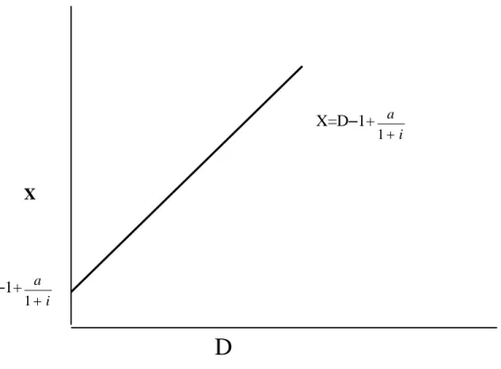
(40) 4.3 The Entrepreneur’ s Decision Problem Following the Miller and Rock (1985) theory, I consider an economy that consists of two time periods.. At the start of period 1, after the earnings and the. dividend/investment/financing decisions have been announced, the cum-dividend value of the shares held by the original owners will be V1=D1+. 1 ~ E( X 2 ) 1 i. = D1+. 1 [F(I1)+γε1] 1 i. (4.8). where i is the appropriately risk-adjusted discount rate for the firm’ s expected earnings; γ is an assumed coefficient of persistence.. Under the standard perfect market/full. information assumptions, a firm operating in the best interest of its current shareholders will choose values of D1, I1 to maximize V1. Different from the Miller and Rock model, this research introduced a general production/investment function to explore the dividend policy and can help to analyze this problem deeper.. Replacing F(I1) with a[ln(I1+1)] and X1-I1 with D1 to rewrite. Equation (4.8), the value of a firm can be expressed as V1=X1-I1+ =D1+. 1 [F(I1)+γε1] 1 i. 1 {aln[(X1-D1+1)]+γε1} 1 i. (4.9) (4.10). 4.3.1 Homogeneous beliefs in the production/investment function We replace V1, D1, X1 with V, D, X, in Equation (4.10). V=D+. 1 {aln[(X-D+1)]+γε} 1 i. (4.11). In order to derive the relationship between X and D for reference (benchmark), we take the first-order derivate to Equating (4.11) and get X＝D－1＋ a. (4.12). 1 i. 34.

(41) Given the MM proposition on dividends, the problem of maximizing the value reduces to decide the optimal investment. I*＝－1＋ a. (4.13). 1 i. The solution is depicted graphically in Figure 4.3.. X=D–1+ a. 1 i. X. –1+ a. 1 i. D Figure 4.3 The relationship between earnings of a firm and cash dividend (homogeneous beliefs). 4.3.2 Heterogeneous beliefs on earning Relaxing the preceding assumption, investors have common information but agree to disagree about the future earnings of a firm.. Divergent investors receive. common information, but differ in the way in which they interpret this information. We assume that there are two types of investors including the optimistic and pessimistic ones.. Each type of investor’ s information is independent of the other. type of investors, and of the common information.. 35.

(42) Investors have heterogeneous beliefs in the future earning of the firm because the investors have different priors, they will interpret information differently. common information, but agree to disagree about X.. They have. The reasons are as follows: a.. People who respect each other’ s opinions and nevertheless disagree about subject probabilities as Aumann (1976) proposed. b. As Gollier (2003) argued, heterogeneity of beliefs does not come from asymmetric information but rather from intrinsic differences in how to view the world.. People agree to disagree, which implies that. prices and observed behaviors of other market participants do not generate any Bayesian updating of individual beliefs. c. Investors share common prior beliefs and receive common information but differ in the way in which they interpret this information.. According to previous assumption, investors receive common information, but differ in the way in which they interpret this information.. The different information. about earnings lead in turn to differences in the perceived value of the firm.. To. model the differences of opinion, we assume that there are two classes (types) of investors agreeing to disagree about the future earnings, with the population of class-i investors being πi ＞0, i=1,2, π 1+π 2=1.. More specifically, class i=o,p.. Recalling. Equation (4.2) V1m =D1+. 1 ~ ｜φm] [ E1m F(I1)+γ  1 1 i. To better understand the effect of heterogeneous beliefs of investors, we sort the market outsider into two types of investors based on V1m. Viewed by optimistic investors, the value of a firm is given by Vo =D+. 1 {ao[ln(X-D+1)]+γε} 1 i. (4.14). For pessimistic investors, the value of a firm is given by Vp =D+. 1 {ap[ln(X-D+1)]+γε} 1 i. (4.15). Equation (4.14) and (4.15) state that the value of a firm is estimated differently by divergent types of investors. assumed to be nonnegative.. The parameter ao estimated by type-o investors is As shown in Figure 4.4, the solution is away from that. 36.

(43) of MM dividend invariance theorem.. The real line depicts the relationship between. earnings X and cash dividend D without considering heterogeneous beliefs of investors; the dotted line is with considering heterogeneous beliefs.. o X=D–1+ a. 1 i X=D–1+ a 1 i. X The MM theorem Heterogeneous beliefs o –1+ a. 1 i –1+ a 1 i. D Figure 4.4 The relationship between earnings of a firm and cash dividend (heterogeneous beliefs). In this case, the firm’ s investment expenditure is increased from (-1+ a ) to 1 i. o (-1+ a ).. 1 i. o (X- a +1).. 1 i. For a given X, the dividend is hence decreased from (X- a +1) to 1 i. The cash dividend paid in difference between the MM theorem and this. case is given by o ΔD=( X- a +1)-(X- a. 1 i. =. 1 i. 1 (ao-a) 1 i. 37. +1).

(44) Where ΔD is the reduction in dividend caused by the heterogeneous beliefs of the optimists, and proportional to the magnitude of ao. of MM dividend invariance theorem.. The result is different from that. Although the slope remains the same, the. intercept is changed. That is, the cash dividend is not a constant but depends on the value of ao.. X X The MM theorem ΔD. ao X+1 1 i. Heterogeneous beliefs. X-. a +1 1 i. D Figure. 4.5 The difference in cash dividend paid between MM and heterogeneous beliefs of investors. To furthermore explore the effect of dividend policy on a firm’ s value, a stronger assumption is made.. We assume that the function of V(D) is concave.. The. following proposition is to derive the relationship between dividend and valuation by different type of investors. Proposition 4.1 The sign of.  Vo  Vp is opposite to that of .  D  D. 38.

(45) Proof. One objective function for the firm compatible with that requirement is a function in which the firm’ s managers attach weights to the interest of each group proportional to the values of their holdings.. The manager’ s problem can then be. written as o p Max V=π 1V +π 2V D. The first-order condition for a maximum with respect to D requires π1.  Vo  Vp +π =0 2  D  D. Re-arranging the preceding equation, we have  Vo  D =- 2  Vp 1  D. (4.16). Because both π1 and π2 are larger than 0 according to the previous assumption, the  Vo  Vp sign of must be opposite to that of .  D  D. Equation (4.16) means as dividend. paid increases, the value of a firm viewed by the optimistic investors increases but decreases by the pessimistic ones. Proposition 4.2 Optimal dividend policy with heterogeneous beliefs of investors is different from that of homogeneous case. Proof.. For the optimistic investors, the value of a firm is given by Vo=D+. 1 {aoln[(X-D+1)]+γε} 1 i. For the pessimistic, the value is given by Vp=D+. 1 {apln[(X-D+1)]+γε} 1 i. The manager’ s problem is described as o p Max V=π 1V +π 2V D. =π1{D+. 1 o a ln[(X-D+1)]+γε} 1 i. +π2{D+. 1 p a ln[(X-D+1)]+γε} 1 i. 39. (4.17).

(46) Taking the first-order partial derivate with respect to D.. Assuming that ao, ap are. independent of D, we have π1{1+[. ao  X ( D) ][ ]} (1 i )( X D 1)  D  D. +π2{1+[. ap  X ( D) ][ ]}=0 (1 i )( X D 1)  D  D. (4.18). Re-arranging the preceding equation, we have π1+π1. ao ao  X -π1 (1 i )( X D 1)  D (1 i )( X D 1). ap ap  X =-π2-π2 +π2 (1 i )( X D 1)  D (1 i )( X D 1) In order to compare dividend policy with heterogeneous beliefs to that of homogeneous one, we collect terms of.  X  D. to the left-hand side of Equation (4.18). and have. ao ap  X [π1 +π2 ]  D (1 i )( X D 1) (1 i )( X D 1) =-π2+π2. ap ao -π1+π1 (1 i )( X D 1) (1 i )( X D 1). Furthermore, we get ao ap 1 2 1 2  X (1 i )( X D 1) (1 i )( X D 1) =  D ao ap 1 2 (1 i )( X D 1) (1 i )( X D 1). 1 2. =1-. 1. ao ap 2 (1 i )( X D 1) (1 i )( X D 1). As known previously, π1+π2=1, the preceding Equation is then reduced to  X =1 D. 1 o. a ap 1 2 (1 i )( X D 1) (1 i )( X D 1). 40. (4.19).

(47) ao ap  X Because π1, π1, and are all positive, must (1 i )( X D 1) (1 i )( X D 1)  D be smaller than 1.. In other words, the slope of the earnings X against dividend D is. not linear the same as that of homogeneous case.. The differences between. heterogeneous and homogeneous case depend on the magnitude of the following term, 1. 1. o. a ap 2 (1 i )( X D 1) (1 i )( X D 1). It is a deviation from that of homogeneous beliefs.. Therefore, optimal dividend. policy with heterogeneous beliefs of divergent investors is different from that of homogeneous case.. Based on previous proposition, we furthermore study the. reasons why heterogeneous beliefs lead in diversity of opinions among investors on a firm’ s future earnings. Proposition 4.3 Optimal dividend policy is changed not only by the ratio of pessimistic to optimistic investors, but also divergent beliefs. Proof.. Based on Equation (4.19), we let F(Io)=. ao ao = (1 i )( X D 1) (1 i )( I 1). (4.20). F(Ip)=. ap ap = (1 i )( X D 1) (1 i )( I 1). (4.21). Divided by (4.20), Equation (4.21) is then reduced to ap F(I )= o F(Io) a p. (4.22). Substituting Equation (4.20) ,(4.21) and (4.22) into the preceding Equation, we have 1+ F(Io) [ =-. 2  X {1+ F(Ip) [ -1]} 1  D. =-. Collecting terms of.  X  D.  X -1]  D. 2 2   X - F(Ip) + 2 F(Ip) 1 1  D 1. to the left hand-side in Equation, we have. 41.

(48) 2 [ F ( I p ) 1] F ( I o ) 1   X = 1   D F (I o )  2 F (I p ) 1 To replace F(Ip) with F(Io), we substitute Equation (4.22) into the preceding one and get. 2 a p [ o F ( I o ) 1] F ( I o ) 1  X  a = 1 2 a p  D o F (I )  F (I o ) o 1 a 2 a p   1]  2 1 1 2 o 1 a 1 1 =1p  a  ap F ( I o )[1  2 o ] F ( I o )[1  2 o ] 1 a 1 a. F ( I o )[. =. Substituting (4.20) into the above Equation, we get  X =1 D.  1 2 1  ap ao (1  2 o ) (1 i )( I 1) 1 a. (4.23). To simply the equation furthermore, we let A=. ap ao. (4.24). C=. 2 1. (4.25). Substituting (4.24) and (4.25) into Equation (4.23), we have  X (1 C ) =1 D F ( I o )(1 CA). (4.26). The result shows that.  X  D. to the optimistic C (=. 2 ap ), but also the beliefs A(= o ). This completes the proof. 1 a. is affected not only by the ratio of pessimistic investors. Then, we check the degree how the ratio of pessimistic to optimistic investors impacts on dividend policy.. 42.

(49) Proposition 4.4 An increase in the ratio of pessimistic to optimistic investors. 2 , 1. that is, pessimistic investors increases will result in a higher dividend. Proof. In order to check the impact of. 2  X (=C) on , we take first-order partial 1  D. derivate with respect to C in Equation (4.26), other things equal, we get  X2  (1 C ) = [1]  D C  C F ( I o )(1 CA) Holding A constant, we take first-order partial derivate with respect to C and have  X 1 = D C F (I o ) 2. (1 CA). =-. 1 (1 CA) A(1 C ) [ ] o F (I ) (1 CA) 2. =-. 1 (1 A) [ ] o F ( I ) (1 CA) 2. There are three conditions of A to influence This case does not exist because assumption..   (1 C ) (1 C ) (1 CA)  C  C (1 CA) 2.  X2 .  D C. (4.27). The first one is that A(=. ap )>1. ao. ap >1 is not reasonable according to the previous ao. Second, when A<1, Substituting into Equation (4.27)  X2 1 (1 A) =[ ] o  D C F ( I ) (1 CA) 2. <0. (4.28).  X2 Because F(I ), A and C are all positive, must be smaller than zero. This means  D C o. that an increase in C(=. 2  X ) will lead in a decrease in . That is, when pessimistic 1  D. investors increase, i.e. a depression in economy occurs, the slope of earnings on dividend.  X becomes flatter than that of normal condition.  D. dividend policy is appropriate to a depression. ap Third, when A(= o )=1 a. 43. We infer that high.

(50)  X2 1 (1 A) =[ ]=0 o  D C F ( I ) (1 CA) 2 The result is the same as that of homogeneous case..  X2  X =0 means that  D C  D. is. not affected by the ratio of the pessimistic investors to the optimistic ones. To summarize, an increase in the ratio of pessimistic to optimistic investors pessimistic investors increases will result in a higher dividend.. 44. 2 , that is, 1.

(51) 4.4 Comparative static analysis Based on proposition 4.2 and 4.3, we furthermore explore the factors to influence the slope of earnings on dividend.  X , and hence to change optimal dividend policy.  D. The results of proposition 4.2 state that optimal dividend policy is different from that of.  X  X =1 because  D  D. is represented by 1. 1-. 1. o. a ap 2 (1 i )( X D 1) (1 i )( X D 1). When existing heterogeneous beliefs among investors,.  X  D. That is, the slope is flatter than that of homogeneous case. is always smaller than 1.  X =1.  D. The degree of. deviation depends on two terms:. ao 1 (1 i )( X D 1) and. 2. ap (1 i )( X D 1). These two terms respectively represent the ratio of optimistic investors to pessimistic ones, and earnings of a firm viewed by theses two divergent investors.. Unlike to. previous research such as Miller and Rock (1985), John and Williams (1987), optimal dividend policy is changed not because of information asymmetry but heterogeneous beliefs.. In addition, optimal dividend policy is changed when considering. heterogeneity among investors not only by the ratio of pessimistic to the optimistic investors. 2 , but also divergent beliefs, ao and ap. This finding has pushed one 1. stage deeper in this topic regarding optimal dividend policy with diversity of opinions. According to proposition 4.4, an increase in ratio of pessimistic to optimistic. 45.

(52) investors will result in a higher dividend.. This is easy to explain.. For a firm’ s. manager, he will shave investment and pay more dividends when a depression occurs. On the other hand, in investors’viewpoints they become more conservative and lead in asking more cash in the form of dividend.. Accordingly, a high dividend is paid. out. This finding is the same as that of previous research work.. However, the. interpretations we propose are very different from the Miller and Rock theory. interpreted a higher dividend policy as a signaling.. They. A good firm must pay a level of. dividends that is sufficiently high to make it unattractive for bad firms to reduce their investment enough to achieve the same level. dividends higher and signal high earnings.. Firms shave investment to make. However, they have not considered the. investors’divergent beliefs.. In order to better understand the impact of the ratio of pessimistic to optimistic investors on.  X  X2 , that is, , we use one example to illustrate.  D  D C. conditions including. Three. 2 2 2  0, =1 and   will be considered as 1 1 1. follows. Condition 1.. 2  0, the investors are 1. When the ratio approaches to zero. almost optimistic. According to Equation (4.23), we get  X =1 D.  1 2 1  ap ao (1  2 o ) (1 i )( I 1) 1 a. 1-. 1 F (I o ). (4.29). Condition 2. When the ratio approaches to 1. are the same as that of pessimistic ones.. 2  0, the optimistic investors 1. Substituting. we have. 46. 2 =1 into Equation (4.23), 1.

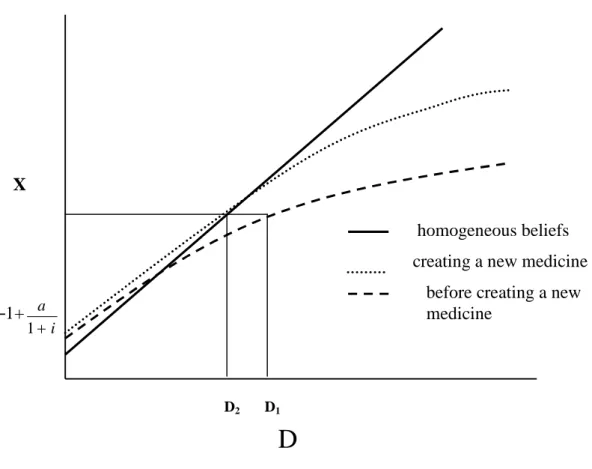
(53)  X =1 D.  1 2 1  ap ao (1  2 o ) (1 i )( I 1) 1 a 1 1. 1-. ap F ( I o )(1  o ) a 2 F ( I ) F ( I p ). =1-. Condition 3. When the ratio approaches to infinite,. almost pessimistic. Substituting. (4.30). o. 2  , the investors are 1. 2   into Equation (4.25), we have 1.  X (1 C ) =1 D F ( I o )(1 CA) 1-. C CAF ( I o ). =1-. 1 F (I p ). (4.31). Comparing Equation (4.29), (4.30) and (4.31), we get 1-. 1 1 1 >1>1o o p F (I ) F ( I ) F ( I ) F (I p ) 2. This means that as the ratio. 2  X approaches to 0, the slope is the largest 1  D. (closest to 1) regardless of what values F(Io) and F(Ip) are. when. Conversely,. 2  X approaches to infinite, is the smallest. To summarize, as pessimistic 1  D. investors increases, i.e. a depression occurs, the slop of earnings on dividends  X becomes flatter than that of homogeneous condition.  D appropriate.. A high dividend policy is. On the contrary, when optimistic investors increase, the slop of earnings. 47.

(54) on dividend becomes steeper.. A low dividend policy is appropriate.. the preceding results graphically in Figure 4.6.. We represent. As shown in the figure, the solution. of heterogeneous beliefs is below the homogeneous beliefs case because.  X  D. must. be smaller than 1.. X. Homogeneous beliefs Heterogeneous beliefs. D0. D1. D Figure 4.6 The solution to heterogeneous beliefs. For a given earnings X, dividend paid out are D0, D1, corresponding to homogeneous and heterogeneous beliefs, respectively.. Apparently, we could find. once a deviation from homogeneous beliefs the firm’ s dividend policy is changed towards higher dividend policy given the same earnings X. the ratio of pessimistic to optimistic investors. towards the right-down direction.. The degree depends on. As the ratio increases, the curve shifts. In managers’viewpoints, more cash is paid out. because there are no investment projects good enough when a depression occurs. This will result in an increase in dividend.. 48. In investors’viewpoints, high dividend is.