行政院國家科學委員會專題研究計畫 期中進度報告
子計畫六:針對先進晶片設計的熱點驗證之完整熱模型與高
效能熱分析(1/3)
計畫類別: 整合型計畫 計畫編號: NSC94-2220-E-009-044- 執行期間: 94 年 08 月 01 日至 95 年 07 月 31 日 執行單位: 國立交通大學電信工程學系(所) 計畫主持人: 李育民 計畫參與人員: 黃至鴻、黃培育、吳佳鴻、林志康、蘇炳熏、簡正忠、于斯安 報告類型: 完整報告 處理方式: 本計畫可公開查詢中 華 民 國 95 年 6 月 1 日
單晶片系統驗證之核心技術開發
子計畫六:針對先進晶片設計的熱點驗證之完整熱模型與高效能熱分析(1/3) Compact Thermal Modeling and Efficient Thermal Simulation
for Hot Spots Verifications of Modern IC Designs
計畫編號:
NSC 94-2220-E009-044
執行期間:94 年 8 月 1 日 至 95 年 7 月 31 日 計畫主持人:李育民 一、中文摘要 當 CMOS 製程技術進步到 100 奈米以下時,隨著元件的密度、操作頻率以及功率消耗 的增加將導致晶片設計上的熱傳問題受到矚目。尤其在先進的系統晶片(SOC)技術及系 統封裝(SIP)中將因為數眾多的熱源積聚於窄小區域內而使的熱傳問題更趨嚴重;此熱 散逸問題在堆疊式封裝(stacked-die package)上尤其明顯。在晶粒疊接(stacked-die) 的幾何架構中,不同的晶片組共用相同的散熱路徑。因此,在晶粒疊接上的累積熱量會 是單晶片(mono-die)上的數倍。如此原本在單晶片上的局部高溫區域極有可能成為熱點 (hotspots)。所以,在最先進的積體電路設計上,有效預測溫度剖面(temperature profile) 的能力將於時序分析、漏電電流抑制、功率估計、熱點避免以及可靠度考量上,扮演一個 十分重要的角色。本計劃的第一年,我們利用一般化的積分轉換(generalized integral transforms)技術針對 設計自動化流程前端發展出一套有效率的熱分析工具。這個分析方法主要是尋找與原系統 方程相容的正交基底(orthogonal bases);當找到這組基底之後,使用葛勒金投影(Galerkin projection)可以將原系統方程轉換成一組無互耦(decoupled)的一維常微分方程式。因為葛勒 金投影只需要積分的運算,此方程式可被很有效率的解決。此方法的執行複雜度與模組的 個數呈線性關係而非格林函數法(Green function)的二次方關係。 關鍵詞:一般化的積分轉換;熱模型;熱分析;熱耦合;溫度剖面;熱點;系統封 裝(SIP);堆疊晶粒 二、英文摘要
As CMOS technology scaled into the sub-100nm region, the increasing component density, operation speed, and power dissipation lead to dramatic thermal problems on chip designs. Furthermore, two of the most advanced chip integration techniques, system-on-chip (SOC) and system-in-package (SIP), will exacerbate the thermal problems because of the accumulation of multiple heat dissipation sources in a small area, and the problems become worse in stacked-die package. In the die stacking geometry, chips are stacked up sharing similar heat dissipation paths as a single die. Thus, the accumulated heat energy in stacked-die is several times than the single chip. The local high temperature region in single chip might become hot spot when the dies are stacked. Therefore, the capability of predicting the temperature profile is critically important for
circuit timing estimation, leakage reduction, power estimation, hotspot avoidance, and reliability concerns during modern IC designs.
In the first year, we develop a generalized integral transforms method to solve the transient and steady temperature distribution for the thermal placement stage. The proposed method first constructs a set of system-compatible orthogonal bases to reduce the variables of original government equation. After those orthogonal bases being constructed, Galerkin projection is utilized to project the original system equations onto a set of reduced-variables equations. Since the Galerkin projection procedure only requires to perform the integral operator through the orthogonal bases and power density of blocks, the computation cost is linearly proportional to the number of blocks.
Keywords:Generalized Integral Transforms, Thermal Model, Thermal Analysis, Thermal Coupling, Temperature Profile, Hotspot, System-in-Package (SIP), Stacked-die
三、研究計畫之背景及目的
As CMOS technology scaled into the sub-100nm region, the increasing component density, operation speed, and power dissipation lead to dramatic thermal problems on chip. For example, chip performance is greatly affected by temperature variation for timing failure - a single inverter is about 35% slower at 110°C than at 60°C; also, chip reliability should be concerned for IR-drop and leakage power – a 30°C change in the temperature will affect the leakage by 30% [1] [2]. Furthermore, hotspots and temperature variations account for over 50% of electronic failures [3]. Therefore, the capability to predict the temperature profile is critically important for circuit timing estimation, leakage reduction, power estimation, and hotspot avoidance. Also, the
temperature-aware design to reduce the performance degradation, such as the thermal placement, is greatly dependent upon thermal simulation [4]-[8]. Therefore, the full chip thermal simulation is necessary for modern VLSI designs.
Several approaches based on numerical or analytical methods have been developed for the thermal analysis. The numerical framework utilizes the finite difference or finite element methods to discretize the heat equation and map the continuous partial differential equation into a large algebra system. With this construction, the heat equation is modeled as a corresponding RC network and the temperature distribution can be computed by MNA (Modified Nodal Analysis) method. Based on the above approach, many numerical simulators are proposed to increase the analyzing efficiency and save the memory usage. The ADI (Alternating Direction Implicit) method is utilized to decompose the equivalent RC kind network into three alternating directions and perform explicit methods at each direction in [9]. Then, the iterative methods are performed for solving the final solution. The IEKS (Improved Extended Krylov Subspace) method is utilized to project the original system into a small system [10]. Hence, the efficiency of simulation can be improved. The hierarchical multi-grid iterative method is proposed to speed up the convergent rate of the basic iterative method [11].
The major advantage of numerical based methods is the flexibility for dealing with the non-homogeneous materials, and this advantage makes the numerical based methods to be the main stream framework at the back-end stage of design flow. However, at the front-end stage, such as the placement stage, due to the lack of the detail information, the chip structure is assumed to be homogeneous [4] [12]. However, even if the homogeneous material of chip is assumed during the thermal placement, the numerical based methods still need to deal with a system with large size. The expensive matrix computation and storage degrade the efficiency and the memory usage of thermal placements. In contrast to the numerical framework, the analytical based framework gains the innate advantage from the homogeneous material assumption. When the material is homogeneous, the approximated response surface of temperature distribution by using the analytical based framework can be calculated without dealing with the equivalent RC network system, and the solution can be explicitly computed. This advantage enhances the efficiency and memory usage during the thermal placement stage.
The Green’s function based analytical simulator for the steady state analysis of the thermal placementhas been proposed in [13] [14]. With the pre-calculated Green’s function, the response surface of temperature distribution can be computed by performing the convolution of Green’s function and power density distribution. Based on the Green’s function formulation, the large lumped system is avoided, and the efficiency and memory usage are enhanced. However, due to the innate property of Green’s function based formulation, i.e. Green’s function is the impulse response respect to the spatial domain, the convolution operator is necessary to find the solution. This factor drops the advantage of the analytical based solver. Furthermore, as dealing with the transient responds of the temperature distribution, the closed form of Green’s function may not easy to be found, and this factor drops the extended potential of Green’s function based formulation. To avoid the convolution operator and extend the analytical based framework to the transient simulation, we proposed a generalized integral transforms method which can efficiently solve the transient and steady temperature distribution at the thermal placement stage.
四、研究方法
The solution flow of the proposed generalized integral transforms based method can be summarized as follows.
‧ System-compatible auxiliary problem construction: At this step, a suitable system-compatible auxiliary problem is utilized to construct the system-compatible orthogonal bases for reducing the number of variables in the original heat equation. Once the system-compatible auxiliary problem is found, the system-compatible orthogonal bases can be pre-calculated.
‧Galerkin projection: After the system-compatible orthogonal bases being constructed, Galerkin projection is utilized to transform the original government equation into a reduced-variable system. Since the Galerkin projection procedure only requires to perform the integral operator through the orthogonal bases and the power density functions of blocks. The computational cost of this step is linearly proportional to the number of blocks.
‧Reduced-variable system computation: Use the numerical based methods to solve the reduced-variable system, and the solution can be constructed by the orthogonal bases and the solution of reduced-variable system. The reduced-variable system is a decoupled system and usually only involves timing variable, and the cost of time step approximation is proportional to the number of system-compatible orthogonal bases.
The rest of this section is organized as follows. In Subsection A, the thermal model of chip die with packaging at the thermal placement stage is introduced, and the algorithm flow of generalized integral transforms method is summarized in Subsection B. Finally, the derivation of computational formula of the whole chip analysis is presented, and the simulation result is presented to demonstrate the accuracy and efficiency in Subsection C.
A. Problem Formulation of the Single Active Layer
(a) … Heat sink Heat spreader Substrate … … Modules Chip die (b)
Lx
Ly
Packaging
z
x
y
Chip die
Z=0
Z=-L
ZModules
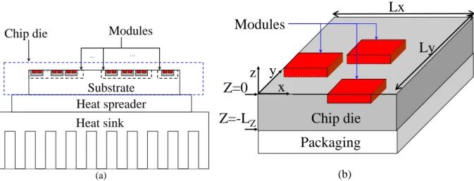
Fig. 1. The schematic structure of VLSI chip with packaging. (a) The cross-section view of chip, heat spreader, and heat sink. (b) The simplified model of the chip.
The structure of VLSI chip and package which consists of modules distributing around the top surface of chip die, and the heat sink and spreader as cooling devices is shown in Fig. 1.a. Because the heat at the bottom surface of chip die can be uniformly distributed by the heat spreader, the packaging can be modeled as an equivalent single package layer with a constant thermal conductivity [15]. Hence, the schematic structure of VLSI chip with packaging can be modeled as Fig. 1.b, and the temperature distribution of chip die with homogeneous material [4] [12] [14] can be governed by the heat diffusion equation as follows.
( )
( )
(
T T r t,)
g r t( )
,( )
T T r t( )
t κ σ ∂ , , ∇ ⋅ ∇ + = ∂ (1)where r=(x, y, z), T(r, t) is temperature ( ) distribution inside the chip at time t, σ(T) is the product
K
(
(
J / m3⋅ K))
of the mass density and the specific heat of chip die, g(r, t) is the power density(
3)
/ m
the chip die. Since the top of chip die is usually covered by a thick and low conductivity oxide layer, the boundary condition at the top surface is assumed to be adiabatic [13]. Due to the chip and package structure, the area of vertical surface is much smaller than the area of horizontal surface, and the conductivity of air is much less than the equivalent package layer. It is reasonable to assume that the boundary condition of vertical surface is adiabatic [13] [14]. If the boundary conditions of the vertical surface of chip die are set to be convective types, our generalized integral transforms method can still work. The initial temperature of chip die is assumed to be the ambient temperature. These boundary conditions and initial condition can be written as
( )
0, ; 0, ; 0 , x y x L y L z T r t n = = = ∂ 0, = ∂ (2)( )
, 0 a, T r =T (3)where Ta is the ambient temperature and
( )
n
∂ ⋅
∂ denotes the partial derivative on the normal direction n of the boundary surface, n is the normal vector of the boundary surface of chip die, Lx
and Ly are the maximum values of the x and y axes of chip die, respectively.
Furthermore, the boundary condition of the bottom surface of chip die can be modeled as a convective type boundary condition with an equivalent convective coefficient h [13]-[15]. It can be written as
( )
,(
( )
,)
z z a z L z L T r t h T r t T z κ =− =− ∂ = ∂ − , (4)where -Lz is the position of the interface between the chip die and packaging with respect to z
B. The Solution Flow of Generalized Integral Transforms ( ) ( )
(
k r)
( ) t ∂ ∇ ⋅ ∇ • + • ∂ System operator Transient analysis Auxiliary problem ( ){
}
N1 i r i φ = Solution representationBy using the normalized spatial bases, the temperature can be written as
( )
, N1 ˆ( ) ( )
i i
i
T r t =
∑
= φ r ψ tThe selected bases by the auxiliary problem
Galerkin projection
…
A small linear system respect to the coefficients
Find solution f Projector g v fgdv ∫ 2( )r φ 1( )r φ φN( )r
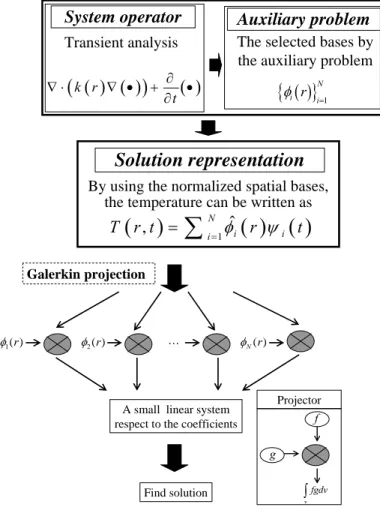
Fig. 2. The flow chart of the generalized integral transforms computation procedure
The computational procedure of generalized integral transforms method is illustrated in Fig. 2. Given the government equation, the system-compatible auxiliary problem is required for generating the appropriate bases. A suitable auxiliary problem needs to contain several features. Firstly, the auxiliary problem should extract as much information as possible from the original problem [16]-[18]. Secondly, the orthogonal bases generated by the auxiliary problem are required to guarantee the convergence in mean property of the approximation of temperature distribution. Furthermore, the orthogonal bases can also effectively simplify the reduced-variables system. Finally, the generated orthogonal bases should be time independent for the efficiency consideration.
After constructing the set of orthogonal bases, the temperature distribution can be expanded by the bases with time varying coefficients. Then, the Galerkin projection is utilized to transform the original four-dimensional (x, y, z, t) problem to one-dimensional (t) problem. Finally, the time step approximation, such as backward Euler and trapezoidal methods, can be used to solve the reduced time variables system. The applications of this technique for IC thermal simulation will be detail discussed in the following subsections.
C. Thermal Simulation of Single Active Layer Chip
The derivation of the computational formula
With assuming the thermal conductivity to be constant and shifting the reference temperature to be zero (T r tˆ
( )
, =T r t( )
, −Ta ), the government Equations (1)-(4) can be transformed to a set of similar thermal equations with homogeneous boundary conditions.( )
( )
( )
2ˆ ˆ , , , T r t g r t T r t t κ∇ + =σ ∂ ∂ , (5.a) 0, ; 0, ; 0 ˆ( , ) 0, x Lx y L zy T r t n = = = ∂ = ∂ (5.b) ˆ( , ) ˆ( , ) , z z z L z L T r t hT r t z κ =− =− ∂ = ∂ (5.c) ˆ( ,0) 0, T r = (5.d)where the notations of Equations (5.a)-(5.d) are the same as the notations in Equations (1)-(4). Because the thermal property of chip material is not time varying during the transient analysis with constant κ assumption, a time independent auxiliary problem can be selected to generate the bases only with respect to spatial dimensions. Hence, the constructed orthogonal bases can be reused during the transient simulation. The construction procedure of auxiliary problem is stated as follows.
Given a set of orthonormal bases
{
φˆ1( ) ( )
r ,φˆ2 r ,...,φˆi( )
r ,...}
with respect to spatial dimensions,the Galerkin projection is performed by multiplying the each basis φˆi
( )
r on both sides of Equation (5.a) and integrating them over the chip die.( )
2( )
( ) ( )
( )
( )
v v v ˆ ˆ , ˆ , ˆ ˆ i r T r t dv i r g r t dv i r T r t dv t φ κ∇ + φ = φ σ ∂ , , ∂∫
∫
∫
v (6) where dv = dxdydz. To include the boundary conditions, the following procedure is required to incorporate the boundary conditions into the transformed problem. By applying Green’s theorem and divergence theorem to(
( ) ( )
)
, andv ˆ ˆ , i r T r t d κφ ∇ • ∇
∫
(
( )
( )
)
v ˆ ˆ i T r r dv κ φ ∇ • ∇∫
, we obtain( ) ( )
(
)
( )
( )
( )
( )
( )
( )
v s 2 v v ˆ ˆ , ˆ ˆ , , ˆ ˆ , ˆ , ˆ i i i i r T r t dv r T r t ds n r T r t dv T r t r dv κφ φ κ φ κ κ φ ∂ ∇ ⋅ ∇ = ∂ = ∇ + ∇ ⋅∇∫
∫
∫
∫
(7)(
( )
( )
)
( )
( )
( )
( )
( )
( )
v s 2 v v ˆ ˆ ˆ , ˆ , , ˆ ˆ ˆ , ˆ , i i i i T r t r dv T r t r ds n T r t r dv T r t r dv κ φ κ φ κ φ κ φ ∂ ∇ • ∇ = ∂ = ∇ + ∇ ⋅∇∫
∫
∫
∫
(8)where
( )
is the surface integration on the boundary surface of simplified chip model.s ⋅ ds
∫
By combining Equations (7) and (8), the first term at the left hand side of Equation (6) is equal to the following form which contains the information of boundary conditions.
( )
2( )
( )
2( )
( )
( )
( )
( )
v v s ˆ ˆ , ˆ , ˆ ˆ ˆ , ˆ , i r T r t dv T r t i r dv i r T r t T r t r ds n n φ κ∇ = κ φ∇ + κ φ ∂ − ∂ φ ∂ ∂ ⎛ ⎞ ⎜ ⎟ ⎝ ⎠∫
∫
∫
ˆ i (9)Since the completed orthogonal property of bases, the solution of Equation (5.a) can be expanded by these bases with time varying coefficients as follows [16] [19].
( ) ( )
1 ˆ ˆ( , ) j j j T r t ∞ φ r ψ t = =∑
(10)Combining Equations (9) and (10) and then substituting them into Equation (6), the transformed problem can be reorganized as follows.
( )
( ) ( )
( ) ( )
( )
( ) ( )
( )
( )
( )
( )
s 2 v v 1 1 ˆ ˆ , ˆ , ˆ ˆ ˆ , ˆ ˆ ˆ , i i j j j j j i i j j r T r t T r t r ds n n r r r t dv r t r dv r g r t κ φ φ φ σ ∞ φ ψ κ ∞ φ ψ φ φ = = ∂ ∂ − ∂ ∂ ⎛ ⎞ ⎛ ⎞ ∂ = ∇ + ⎜ ⎟ ⎜ ⎟ ∂ ⎝ ⎠ ⎝ ⎠ ⎛ ⎞ − ⎜ ⎟ ⎝ ⎠∫
∑
∑
∫
∫
∫
v t dv)
(11)The representation of in Equation (10) doesn’t involve the surface integration since the term of the surface integration in Equation (11) can be eliminated by chosen appropriate bases (
(
ˆ , T r t( )
ˆ i rφ ’s). By observing Equation (11), if the bases satisfy the following property, Equation (11) can be further reduced.
2ˆ 2 ˆ ( ) ( ) 0 i r i i r φ λ σφ ∇ + = (12.a) (12.b) v 1 ; ˆ( ) ( )ˆ 0 ; i j i j r r dv i j φ φ = ⎨⎧ = ≠ ⎩
∫
0, ; 0, ; 0 ˆ ( ) 0 x y i x L y L z r nφ = = = ∂ = ∂ (12.c) ˆ( ) ˆ( ) z z i i z L z L r h r z κ φ φ =− =− ∂ = ∂ (12.d)According to Equations (12.a) and (12.b), each must be the eigenfunction of the Laplacian operator and λ
ˆ ( )i r
φ
i be the corresponding eigenvalue, and the bases are orthonormal. With
applying Equations (12.a) and (12.b) to Equation (11), the first term at the right hand side of Equation (11) is equal to (13)
( ) ( )
2( )
( )
v 1 ˆ ˆ . j j i i i j r t r dv k t κ ∞ φ ψ φ λ ψ = ⎛ ⎞ ∇ = − ⎜ ⎟ ⎝∑
⎠∫
2The left hand side of Equation (11) can be decoupled by using Equation (12.b) as follows.
( )
( ) ( )
( )
v 1 ˆ ˆ , j j j j r r r t dv t t φ σ ∞ φ ψ σ ψ = ⎛ ⎞ ∂ = ⎜ ⎟ ∂ ⎝∑
⎠ ∂∫
i t ∂ (14)Furthermore, the surface integration in Equation (11) can be eliminated from Equations (12.c) and (12.d). The verification is stated as following.
Multiplying Equation (5.c) by φˆ ( )i r and Equation (12.d) by T r tˆ
( )
, , respectively, we can obtain the following equations.( )
( )
( ) ( )
ˆ ˆ , ˆ ˆ , z z i i z L z L r T r t h r T r t n κ φ φ =− =− ∂ = ∂ (15.a)( )
ˆ( )
ˆ( ) ( )
ˆ , ˆ , z z i i z L z L T r t r h r T r t n κ φ φ =− =− ∂ = ∂ (15.b)Subtracting Equation (15.a) from Equation (15.b), we have
( )
( )
( )
( )
ˆ ˆ , ˆ , z z i z L z L r T r t T r t r n n κ φ φ =− =− ⎛ ∂ ∂ ⎞ − ⎜⎜ ∂ ∂ ⎝ ⎠ ˆ 0 i ⎟⎟= = (16)Therefore, the surface integration in Equation (11) can be eliminated. Finally, the initial condition of Equation (5.a) can be represented as
(17)
( )
( ) ( )
1 ˆ , 0 0 0 j j j T r ∞ φ r ψ = =∑
With multiplying Equation (17) by and integrating it over the chip die, we can get the initial condition of i
ˆ ( )i r
φ th
time varying coefficient. Hence, the original system can be simplified to a decoupled and reduced-variable system with respect to time varying coefficients.
( )
( ) ( )
( )
2 v ˆ , i i i i k t r g r t dv t t λ ψ φ σ ψ∂ , i − + = ∀ ∂∫
(18.a)The initial condition of Equation (18.a) can be computed as
( )
0 0,i i
ψ = ∀ . (18.b)
Since ψi(t) is independent of other ψj(t)’s as shown in Equations (18.a) and (18.b), each ψi(t) can
be solved independently, and this kind of system is called decoupled system. Since this decoupled system only involves the time varying variables, the numerical method can be utilized to solve it efficiently. The bases satisfying Equations (12.a)-(12.d) are the solutions of the first class of Strum-Liouville problem, and the solving procedure can be found in [9]. After constructing the general form of reduced-variable system, a real case application of thermal simulation is given in the next subsection.
Real Case Thermal Simulation
Fig. 3. Topology of DEC Alpha 21264 chip [20].
In this section, we use the DEC Alpha 21264 chip [20] as the test case and compare the simulated temperature distribution with the widely used industrial tool, ANSYS, for verifying the accuracy. The topology of DEC Alpha 21264 chip is shown in Fig. 3. Each block indicates a module accompanied with a given power density. Our proposed thermal solver is used to obtain the temperature distribution of this chip. Based on the literature [16], we can find bases satisfying the Equations (12.a)-(12.d) as follows.
( )
, ,(
)
1( )
2
1
ˆ ˆ , , cos cos cos ,
i n m l l x y i m x n y r x y z L L N π π φ =φ = ⎛⎜ ⎞⎟ ⎛⎜⎜ ⎞⎟⎟ η ⎝ ⎠ ⎝ ⎠ z (19) where
(
)
(
)
(
)
2 2 2 2 2 2 1 sin ; 0, 0 2 1 sin ; 0, 0 0, 0 , 4 1 sin ; 0, 0 8 x y z z l l z i x y z z l l z x y z z l l z L L L L L if m n h h N L L L L L if m n or m n h h L L L L L if m n h h κ κ η η κ κ η η κ κ η η ⎧ ⎛ ⎛ ⎞ ⎞ + + = = ⎪ ⎜⎜ ⎜ ⎟ ⎟⎟ ⎝ ⎠ ⎪ ⎝ ⎠ ⎪ ⎛ ⎞ ⎪ ⎛ ⎞ =⎨ ⎜⎜ + + ⎜⎝ ⎟⎠ ⎟⎟ = ≠ ≠ ⎪ ⎝ ⎠ ⎪ ⎛ ⎞ ⎛ ⎞ ⎪ ⎜ + + ⎟ ≠ ≠ ⎜ ⎟ ⎪ ⎜⎝ ⎝ ⎠ ⎟⎠ ⎩ = (20)(
cot . l lLz)
h κ η = η (21)The m, n, l are integers, and ηl can be obtained by using the Newton-Raphson method [21]. Each
eigenvalue, λi, is equal to 2 2 2 2 , , . i m n l l x y m n L L π π 2 λ =λ =⎛⎜ ⎞⎟ +⎛⎜⎜ ⎞⎟⎟ + ⎝ ⎠ ⎝ ⎠ η (22)
We then compute the bases with respect to the average power density integration of each module in Equations (18.a)-(18.b). Due to the observation that the integration of average power density of each module is only a function of time, we re-define the basis of average power density
integration of each module as .
( )
( ) ( )
(23) v ˆ , i i g t ≡∫
φ r g r t dvBy using the assumption that the average power density of each module is uniform but different [13] [14], we can rewrite the Equation (23) and integrate over each module as follows.
( )
(
)
(
)(
)
( )
, ,
1 1
( ) bR bu bt avg cos cos cos ,
bL bd bb R L u d t b B x y z b i i m n l x y z l b b b b b b b x y i P t m x n y g t z dzdydx x x y y z z L L N π π η ← = ≡ − − − ⎛ ⎞ ⎛ ⎞ ⎜ ⎟ ⎜ ⎟ ⎝ ⎠ ⎝ ⎠
∑∫ ∫ ∫
(24)where b is the index of each module, |B| is the number of module, and are the maximum
and minimum value of the b
R b x L b x th
module in x-axis, respectively, and are the maximum
and minimum value of the b
R b y L b y th
module in y-axis ,respectively, and are the maximum
and minimum value of the b
R b y L b y th
module in z-axis, respectively, and
( )
avgb
P t is the average power
of bth module. The definition of each parameter is shown in Fig. 4.
Substrate L b x R b x d b y u b y t b z b b z The active region of modulesbth
Fig. 4. The geometrical illustration of bth module. After computation, Equation (24) can be rewritten as
( )
( )
(
)
(
)
( )
(
)
(
)
(
)
(
)
( )
(
) (
)
(
)
(
)
( )
(
)
(
)
1 1 , , 1 , 1 ; 0, 0 , , 1 ; 0, 0 , , 1 ; 0, 0 , , 1 avg t b t b avg R L t b R L t b avg R d t b R L t b avg R L R d B b l b b b l b b B x b m b b l b b b l b b b b m n l B y b n b b l b b b l b b b b x y b m b b n b b i i i i P t S z z m n z z L P t S x x S z z m n m x x z z g t L P t S y y S z z m n n y y z z L L P t S x x S y yN
N
N
N
η η π η π = = = = = − ≠ = − − = = ≠ − −∑
∑
∑
(
)
(
)(
)(
)
2 1 , , ; 0, 0 t b R L R L t b B l b b b l b b b b b b S z z m n mn x x y y z z η π = ⎧ ⎪ ⎪ ⎪ ⎪ ⎪ ⎪⎪ ⎨ ⎪ ⎪ ⎪ ⎪ ⎪ ≠ ≠ ⎪ − − − ⎪⎩∑
(25.a) where(
,)
sin( )
sin( )
(25.b) t b t b l b b l b l b S z z =⎡⎣ ηz − ηz ⎤⎦ ,(
,)
sin R sin R L b m b b x x m x m x S x x L L π π ⎡ ⎛ ⎞ ⎛ ⎤ =⎢ ⎜ ⎟− ⎜ ⎢ ⎝ ⎠ ⎝ ⎥ ⎣ ⎦, L b ⎞ ⎥ ⎟ ⎠ (25.c)(
,)
sin R sin d R d b b n b b y y n y n y S y y L L π π ⎡ ⎛ ⎞ ⎛ ⎤ =⎢ ⎜⎜ ⎟⎟− ⎜⎜ ⎢ ⎝ ⎠ ⎝ ⎥ ⎣ ⎦ . ⎞ ⎥ ⎟⎟ ⎠ (25.d)After obtaining the value of
( ) ( )
v
ˆ ,
i r g r t dv
φ
∫
by using the above computation, the trapezoidal approximation can be utilized to obtain ψi(t) in Equations (18.a)-(18.b). The computationprocedure is presented as follows. Equation (18.a) can be rewritten as
(
2 2 2 2 1 , 2 2 t i t h t i i i i i h g g h h σ λ κ t h)
i ψ ψ σ λ κ σ λ κ − − = + + + − + (26)where h is the sampling time step, ψ and it ψit−h are the time variables of ith basis
corresponding to time step t and t-h, g~it and g~it−h are the ith basis corresponding to the average power density integration at time step t and t-h. By using Equations (10), (19)-(22) and (26), the temperature distribution of the chip die can be expressed as
( )
( ) ( )
(27) 1 ˆ ˆ( , ) ˆ , M , M j j T r t T r t φ r ψ t = ≅ =∑
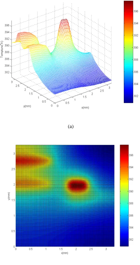
j(a)
(b)
Fig. 6. Steady state temperature distribution. (a) The cross curve of temperature distribution at the top surface of test chip. (b) The contour of temperature distribution at the top surface of test chip.
algorithm. For the transient simulation, we perform 1000 time step analysis by using Equation (26). The maximum error is about 1% compared with the result of Ansys at each time step, and the truncated number of bases is 1600. The run time for computing the steady state temperature distribution is 0.3 second, and the memory usage is less then one mega bytes. The computed steady state temperature distribution of the test chip is shown in Fig. 6. The computation efficiency is hundreds of times better than the finite-element based commercial tool Ansys.
五、結論與討論
In this report, we have developed a general integral transforms based method to analyze the thermal distribution of the full chip. The result shows that the proposed method is very efficient and accurate. We will extend this method to deal with the chip structure with multi-substrate layers (3-dimensonal ICs).
At the end of this report, let’s discuss the issues as we implement Equations (19)-(27) and how to overcome them. We illustrate the problems first, and then deal with them to speed up the convergent rate.
If the desired approximation number of bases, M, is 64, the maximum error at each time step is about 2% compared with the result of Ansys. However, the maximum error is slightly reduced to 1% even if M reaches 1000.
This observation shows that increasing the number of bases only slightly reduces the error. To find why it occurs, we analyze the relation of convergent rate between error and the number of bases. By subtracting Equation (10) from Equation (27), squaring the subtracting result and integrating over the whole chip, we have
(
( )
( )
)
2( )
( )
v ˆ , ˆ , ˆ , ˆ , M v T r t −T r t dv≡ T r t −T r t∫
2 . N (28)Then, by comparing it with Equation (10), the error can be obtained as follows.
( )
( )
( )
2 2 , , . , N v v T r t T r t Error T r t − = (29)( )
( )
( )
( )
( )
( )( )
( )
( )( )
( )
( )( )
( )
( )( )
( )
( )
( )( )
2 2 2 2 2 2 2 2 2 0 1 2 0 1 2 0 i= +1 2 0 i=1 0 i= +1 , , , ˆ ˆ ˆ ˆ ˆ ; ˆ i i i i i i N v v t t i i i M v t t i i i v t t i v i M i j t t i v i t t i M t i T r t T r t Error T r t r g e d r g e d r g e d r r r g e d g e d g e λ τ λ τ λ τ λ τ λ τ λ φ τ τ φ τ τ φ τ τ φ φ φ τ τ τ τ τ ∞ − − = + ∞ − − = ∞ − − ∞ − − ∞ − − − − − = = = ⊥ =∑
∫
∑
∫
∑
∫
∑
∫
∑ ∫
∵ ( )( )
(
)
(
( ))
( )
(
)
(
( ))
( )
(
)
( )
(
)
( )
2 2 0 i=1 1 1 2 2 2 2 0 0 i=M+1 1 1 2 2 2 2 0 0 i=1 1 1 2 2 2 0 i=M+1 1 1 2 2 2 0 i=1 2 2 2 , , ; by Cauchy-Swaiz inequality i i t t t t i t t t i t i i t i i m n l l l x y d g d e d g d e d g d g d m n g t L L τ λ τ λ τ τ τ τ τ τ τ τ λ τ τ λ τ τ π π η ∞ ∞ − − ∞ − − ∞ ∞ ≤ ≤ ⎛ ⎞ ⎛ ⎞ +⎜ ⎟ + ⎜ ⎟ ⎜ ⎟ ⎝ ⎠ ⎝ ⎠ =∑∫
∑ ∫
∫
∑ ∫
∫
∑
∫
∑
∫
( )
1 1 1 2 2 2 . . 1 1 1 . m i n j k m n l l m n l x y m n g t L L π π η ∞ ∞ ∞ = + = + = + ∞ ∞ ∞ = = = ⎛ ⎞ ⎛ ⎞ +⎜ ⎟ + ⎜ ⎟ ⎜ ⎟ ⎝ ⎠ ⎝ ⎠∑ ∑ ∑
∑∑∑
(30)From Equation (30), we find that the error is related to the power of the interception of bases. The reason why the error doesn’t be significantly reduced as we use large number of bases is resulted from the discontinuous of power density distribution.
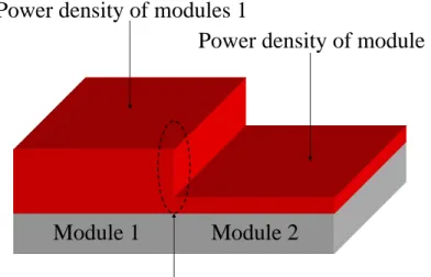
Module 1
Module 2
Power density of modules 1
Power density of module 2
The discontinue junction of power density
Fig. 5. Power density distribution of two modules
The power densities of two modules are shown in Fig. 5. Obviously, the power density is discontinuous at the interface of two modules. Because Equations (25.a)-(25.d) are the projections of power density of each module on each basis, and each basis is a sinusoidal form, the so-call Gibb’s phenomenon at discontinuous site can result in significant error. To solve this problem, we plan to use Bell’s function in the wavelet theory [22]-[24] to smooth the discontinuity at the interface, and then use the smooth local wavelet bases to span Bell’s function. After performing this procedure, the projection of Equations (25.a) to (25.d) will be continuous. Due to the continuous relation, the Gibb’s phenomenon will be eliminated. Therefore, the error will be reduced and the convergent rate will be improved. This technique is still under construction. Although with the influence of Gibb’s phenomenon, our original solver, without using the wavelet theory, still provides good accuracy with comparison to the industrial software, Ansys, and the computationalefficiency is hundreds of times better than Ansys.
六、成果
[1] Pei-Yu Huang, Yu-Min Lee, Jeng-Liang Tsai, and Charlie Chung-Ping Chen,
‘‘Simultaneous Area Minimization and Decaps Insertion for Power Delivery Network Using Adjoint Sensitivity Analysis with IEKS Method”, IEEE International Symposium
on Circuits and Systems (ISCAS), May 2006.
[2] Yih-Lang Lin, Pei-Yu Huang, and Yu-Min Lee, ‘‘Performance- and Congestion-Driven Multilevel Router”, The 13th Workshop on Synthesis and System Integration of Mixed
Information Technologies (SASIMI), April 2006.
[3] Pei-Yu Huang, Chih-Kang Lin, Jia-Hong Wu, and Yu-Min Lee, ‘‘IC Thermal Analysis via Generalized Integral Transforms”, will be submitted to Asia South Pacific Design
Automation Conference (ASP-DAC) 2007. (will be submitted)
七、參考文獻
[1] Ajami A. H., and Banerjee K., “Analysis of IR-drop Scaling with Implications for Deep Submicron P/G Network Designs”, International Symposium on Quality Electronic
Design (ISQED), pp. 35-40, 2003.
[2] Haihua Su et. al., “Full Chip Leakage Estimation Considering Power Supply and Temperature Variations”, International Symposium on Low Power Electronics and
Design (ISLPED), pp. 78-83, 2003.
[3] L. T. Yeh, and R. C. Chu., “Thermal Management of Microelectronic Equipment: Heat Transfer Theory, Analysis Methods and Design Practices”, ASME Press, New York, NY, 2002.
[4] Ching-Han Tsai, and Sung-Mo Kang, “Cell-level Placement for Improving Substrate Thermal Distribution”, IEEE Transactions on Computer-Aided Design of Integrated
Circuits and Systems (TCAD), vol. 19, no. 2, pp. 253 – 266, 2000.
[5] Ching-Han Tsai, and Sung-Mo Kang, “Standard Cell Placement for Even On-chip Thermal Distribution”, International Symposium on Physical Design (ISPD), 1999. [6] Obermeier, B., and Johannes F.M., “Temperature-aware Global Placement”, Asia
and South Pacific Design Automation Conference (ASP-DAC), pp. 143 – 148, 2004.
[7] Guoqiang Chen, and Sachin Sapatnekar, “Partition Driven Standard Cell Thermal Placement”, ACM International Symposium on Physical Design (ISPD), 2003.
[8] Chris C. N. Chu, and D. F. Wong, “A Matrix Synthesis Approach to Thermal Placement”, IEEE Transactions on Computer-Aided Design of Integrated Circuits and
Systems (TCAD), vol. 17, no. 11, 1998.
[9] Ting-Yuan Wang and Charlie Chung-Ping Chen, ”Thermal-ADI:A Linear-Time Chip-Level Thermal Simulation Algorithm Based on Alternating-Direction Implicit (ADI) Method”, in IEEE Trans. on Very Large Scale Integration Systems (TVLSI), Vol. 11, No. 4, pp. 691-700, Aug. 2003.
[10] Ting-Yuan Wang and Charlie Chung-Ping Chen, ”SPICE-Compatible Thermal Simulation with Lumped Circuit Modeling for Thermal Reliability Analysis based on Model Reduction”, in 5th International Symposium on Quality Electronic Design
(ISQED), 2004.
[11] Peng Li, L. T. Pileggi, M. Asheghi, and R. Chandra, ”Efficient Full-Chip Thermal Modeling and Analysis”, in International Conference of Computer-Aided
[12] B. Goplen and S. S. Sapatnekar, ”Efficient Thermal Placement of Standard Cells in 3D ICs Using a Force Directed Approach”, in International Conference on
Computer-Aided Design(ICCAD), pp. 86-89, 2003.
[13] Y. Zhan and S. S. Sapatnekar, ”A High Efficiency Full-Chip Thermal Simulation Algorithm,” in Proc. of the IEEE/ACM International Conference on Computer-Aided
Design(ICCAD), pp. 634-637,2005.
[14] Y. Zhan and S. S. Sapatnekar, ”Fast Computation of Temperature Distribution in VLSI Chips Using the Discrete Cosine Transform and Table Look-up”, in Proc .of Asia
and South Pacific Design Automation Conference(ASPDAC), pp. 87-92, Jan. 2005
[15] Y. K. Cheng, P. Raha, C. C. Teng, E. Rosenbaum, and S. M. Kang, ”ILLIADST: An Electro-thermal Timing Simulator for Temperature Sensitive Reliability Diagnosis of CMOS VLSI Chips”, in IEEE Trans. Computer-Aided Design Integr. Circuits
Syst.(TCAD), vol. 17, no. 8, pp. 668-681, Aug. 1998.
[16] M. D. Mikhailov and M. N. Ozisik, Unified Analysis and Solutions of Heat and Mass Diffusion. N.Y.: John Wiley & Sons Inc., 1983.
[17] R. M. Cotta, Integral Transforms in Computational Heat and Fluid Flow. Florida:
CRC Press Inc., 1993.
[18] R. M. Cotta, M. D. Mikhailov and M. D. Mikhailov, Heat Conduction: Lumped Analysis, Integral Transforms, Symbolic Computation. N.Y.: John Wiley & Sons Inc., 1997.
[19] Chi Y. Lo, ”Boundary VALUE PROBLEM”, World Scientific Publishing Co. Pte.
Ltd, 2000.
[20] W. Liao, L. He, and K. Lepak, “Temperature-Aware Performance and Power Modeling”, Tech. Report UCLA Engr., 04-250, UCLA, CA, 2004.
[21] W.H. Press, S. A. Teukolsky, W. T. Vetterling, and B. P. Flannery, “Numerical Recipes in C++”, Cambridge Unvi. press, 2002.
[22] C. K. Chui, “An Introduction to Wavelet”, Academic Press, 1992.
[23] G. String and T. Nguyen, ”Wavelets and Filter Banks”,Wellesley- Cambridge, 1996. [24] G. W. Pan, Y. V. Tretiakov, and B. Gilbert, “Smooth Local Cosine Based Galerkin
Method for Scattering Problem”, in IEEE Trans. Antennas and Propagation, vol. 51, no. 6, June 2003.
![Fig. 3. Topology of DEC Alpha 21264 chip [20].](https://thumb-ap.123doks.com/thumbv2/9libinfo/8368336.177341/11.892.293.574.108.373/fig-topology-dec-alpha-chip.webp)