結構健康診斷及控制研究--大型結構實驗驗証---子計畫：應用類神經網路技術於房屋結構之非線性系統識別、損壞診斷以及健康監測(I)

行政院國家科學委員會補助專題研究計畫

█ 成 果 報 告

□期中進度報告

結構健康診斷及控制研究:大型結構實驗驗証--子計畫：應用類神經網路技

術於房屋結構之非線性系統識別、損壞診斷以及健康監測(I)

計畫類別：□ 個別型計畫 █ 整合型計畫

計畫編號：NSC

93-2625-Z-009-005-

執行期間： 2004 年 8 月 1 日 至 2005 年 12 月 31 日

計畫主持人：

洪士林

共同主持人：

計畫參與人員：林子軒、林宏宇

成果報告類型(依經費核定清單規定繳交)：□精簡報告 █完整報告

本成果報告包括以下應繳交之附件：

□赴國外出差或研習心得報告一份

□赴大陸地區出差或研習心得報告一份

█出席國際學術會議心得報告及發表之論文各一份

□國際合作研究計畫國外研究報告書一份

處理方式：除產學合作研究計畫、提升產業技術及人才培育研究計畫、列

管計畫及下列情形者外，得立即公開查詢

□涉及專利或其他智慧財產權，□一年□二年後可公開查詢

執行單位：

國立交通大學土木工程學系

中 華 民 國 九十五 年 三 月 三十一 日

中文摘要

以往結構耐震設計之觀念已逐漸由韌性設計慢慢轉變為功能設計（performance design）， 而對結構之功能要求也逐漸朝向智慧型結構（intelligent structure）來發展。結構健康監測系 統（structural health monitoring system）為掌握智慧型結構之生命週期中結構安全性的重要關 鍵，因此近二十年來，關於此議題的研究逐漸的被地震工程研究人員所重視並蓬勃地進行。 在一完善的結構健康監測系統之中，破壞檢測系統（damage detection system）主宰了結構體 之安全與維護之功能，當結構體因材料之退化或是因強大外力之作用下而產生破壞時，良好 的結構破壞檢測系統能夠根據適當的量測資料適時發出破壞發生之警訊，同時提供破壞之位 置並評估破壞的程度等訊息，以供維修人員對該結構進行適當之處置。 此外，台灣地處板塊交接處且島內分佈多條地震發生頻繁的斷層帶，每年發生的大小地 震不勝枚舉，當較大的地震發生時，結構系統便可能會產生非線性的行為。而結構系統之非 線性行為往往主宰了結構系統的安全問題，因此，若能經由對結構非線性行為模式之識別， 便能更準確的分析與預期結構的非線性行為，也就愈能掌握結構在較大地震中的動態反應而 達到降低結構不安全的疑慮。 因此，本研究配合台大羅俊雄 教授向國科會永續會所提之整合型計畫－「結構健康診斷 及控制研究：大型實驗驗證」，將研究之重點著重在房屋結構破壞檢測系統之開發，以及結 構系統非線性行為之識別兩個方面，以期透過這兩個研究主題，建立結構體安全監測系統之 架構。本計畫將以人工智慧中應用相當成功的類神經網路，作為發展結構非線性系統識別模 型、結構之損壞診斷、狀況評估的工具。本研究配合國科會永續會之整合型計畫之分年研究 重點，預計以三年的時間進行相關研究工作，本計畫為第一年度之研究案。所需之試體結構 為國家地震工程研究中心（NCRE ）設計之Benchmark Model ，該Benchmark Model 將於中 心之地震模擬振動臺上進行相關之動力實驗。

ABSTRACT

The concept of the structural seismic design has gradually been changed from ductility design to performance design. And the desire for the intelligent structures is progressively growing. The structural health monitoring system is the key to maintain the safety and reliability of the structure in the structural life cycle. Therefore, during the recent two decades, more attentions are focus on the structural health monitoring related studies by the seismic engineering researchers. In an ideal structural health monitoring system, the damage detection subsystem dominates the safety and maintenance functions of the structure. When a structure is damaged because of the degradation of material or the excitation impact, a well-organized structural damage detection system is capable of making a warning when damage(s) occurred according to the measured information on the structure. Besides, the system can identify the damage location(s) and evaluate the extent(s) of the damage(s). The information from the damage detection system is the basis for the maintenance workers to make the appropriate treatments to the structure.

Taiwan is located on the fault area where the earthquakes are frequently occurred. The earthquake events that happened to this island usually exceed hundreds in every year. When an earthquake with higher intensity excites a structure, the structure may have nonlinear behavior. The nonlinear behavior of a structure system is usually the key point to the safety of the structure. With more accurate identification of the nonlinear structure system, the response of the nonlinear system can be more accurately analyzed and predicted to reduce the misgivings of structural safety when the structure suffers a larger excitation.

Consequently, cooperating with the integrated project of NCSD that is originated by Prof. Loh, a three-year subproject that is drafted by the author will focus efforts on two major topics: the development of the structural damage detection system; and the identification of the nonlinear behavior of the structure system. With the studies in two topics, a frame of the structural health monitoring system is anticipant to be established. The ANN is used as a tool to develop the nonlinear SI model, damage detection approach, and condition assessment method in this subproject. This proposal is the description about the first year study of the

three-year subproject.

Keywords：intelligent structure, health monitoring, damage detection, system identification, structural nonlinear response, artificial neural networks

壹、前 言

結構動力學發展至今雖已相當完備，然而由於近年來結構物加裝了一些隔減振的裝置加 上施工的不確定導致結構物震動的行為更加複雜難分析，這樣將導致結構物之理論分析與實 際結果之間有相當的差異。複雜結構的實際行為，一般不易由理論分析而獲得。因此，為能 瞭解實際結構之真實特性，吾人常利用強迫振動等方式進行結構模態試驗，以瞭解結構的動 力特性。 結構材料之退化或是強烈外力如大地震之侵襲後，便有可能使結構物遭受到損壞。而傳 統上，對於結構物之評估多藉由目測診斷。然此法較不符合經濟之效益。近年來，許多創新 的感應器技術陸續地被發展出來，並應用在建築或土木結構之監測上。藉由感應器適當的布 置，測量結構在震動下的結構反應資料，吾人便可依據這些量測的資料的分析結果，評估結 構是否發生破壞，或更進一步地瞭解這些破壞的一些特性。

1.1、文獻回顧

系統識別若依其所用模式，可概分為： 1. 參數識別法：即利用一有限維數之參數向量，描述輸出與輸入之關係，ARX、ARMAX、狀 態空間模式、以及本文所提識別程序。 2. 非參數識別法：假設對於系統的輸出和輸入，可以用一組相關函數表示之間的關連，函 數的係數即是要識別的。如一般之識別頻率響應函數[1]。 若依分析方法，約可分為頻率域與時間域分析兩大類。頻率域分析[2]發展較早也較為方 便，但是較不適用於非線性及時變系統，且對於高阻尼與模態干擾較嚴重之線性非時變系統 的識別能力較差。若依量測數據之處理程序，則系統識別技巧亦可概分成兩類：（1）線上模 式（on-line model）及（2）離線模式（off-line model）。線上模式乃於數據進來一筆；即 進行系統識別一次，其分析技巧架構於遞迴公式（recursive formula）[3]。而離線模式， 則於所有數據集錄完成，再進行系統識別。線上分析模式，雖有減少數據儲存時間、計算快 速及可分析時變系統之優點，但於分析線性非時變系統，則其精度一般不如離線分析模式。 另外，線上分析模式於決定模式階數不若離線分析模式方便。本文所用分析方法，即為離線 者。 在同時利用系統輸入及輸出量測數據下，ARX 與 ARMAX 時間序列模式即為常被應用之時 間域分析法。在許多教科書[1, 3, 4~5]及論文[6~13]，描述各種估算 ARX 與 ARMAX 模式係數

之方法。但是，卻少有應用於土木工程。鑑於近幾年土木工程監測之必要性逐漸被重視，此 些方法已成功地應用於土木工程[14~18]，由於估算方法之多樣性，有些專家學者即針對各種 方法進行比較，如 Yun 和 Shinozuka [19]則針對傳統最小平方差法、工具變數法、最大可能 機率法(maximum likelihood algorithm)和有限訊息最大可能機率法(limited information maximum likelihood method)應用於多重輸入╱輸出系統建立 ARX 模式之比較。Ghanem 和 Shinozuka [16、20]亦對推廣卡氏過濾法(entended Kalmen filter algorithm)、最大可能 機率法、遞迴最小平方差法(recursive least square method)、和遞迴工具變數法應用於多 重輸入╱輸出系統建立 ARX 模式比較。Saridis [21]針對線上分析法之互相關法（cross correlation algorithm ）、 一 階 隨 機 近 似 法 （ first order stochastic approximation algorithm）、二階隨機近似法(second order stochastic approximation algorithm)、最大 可能機率法、最大事後機率法（maximum posteriori probability algorithm）、推廣卡氏過 濾法應用於線性單一輸入╱輸出系統(SISO)之比較。

在過去的二十年間，類神經網路（ANN）逐漸地發展成熟並應用在許多的領域之中。由於 類神經網路強大的學習能力，及其對於部分不精確資料的高容錯性，使其無論在模式識別 （pattern recognition）、訊號處理（signal processing）、控制、以及複雜的映射（mapping） 等問題上，成為了一種強有力的應用工具。而最近幾年，類神經網路更進一步地被應用在結 構的破壞評估上。Wu 等人[22]以一系列三層樓鋼構架之數值模擬資料，利用倒傳遞神經網路 （back-propagation neural network, BPN）來描述該結構的破壞狀態。該研究以加速度反 應富氏譜以及桿件勁度，分別作為其 BPN 之輸入及輸出變數。而 Elkordy 等人[23]則以模態 作為其 BPN 之輸入變數，以偵測模擬的結構破壞。Szewczyk 與 Hajela [24]則應用反傳遞神 經網路（counter-propagation neural network, CPN），以剛架之靜定位移來估算桿件勁度 的折減情形。Pandey 與 Barai [25]應用多層感知器（multilayer perceptron），以數值模擬 資料偵測桁架橋之破壞。Zhao 等人[26]以靜定位移、自然頻率、以及模態，應用 CPN 來分別 偵測梁和剛架的破壞位置。Masri 等人[27]根據非線性系統識別，建立了一套破壞偵測的方 法。其方法裡採用了實驗中所量測到的位移、速度、加速度反應，以及輸入外力等資料，作 為網路訓練之用。

1.2、研究方法

本研究僅使用加速度反應以及輸入地表加速度資料作為網路訓練之用。本報告中，提出 了一套從已訓練網路的權植，來估算系統之動力特性如自然頻率、振態阻尼比、以及模態的

系統識別程序。 本研究將首先以數種型式的 Benchmark 模型於振動台上量測的反應作為案例，來驗證所 提出之系統識別程序。以多種不同強度下的地震力有線性與非線性的測試作為震動台輸入力 源，進而量測其各樓層之結構反應。程序驗證的步驟概述如下： 1. 利用 Benchmark 實驗資料訓練類神經網路。 2. 根據網路收斂情形，就其網路架構做適當的修正。 3. 由訓練完成的網路權重矩陣估算結構之模態參數。 4. 將實際數據與分析結果做比較，以驗證所提方法之可行性。

貳、類神經網路

2.1、倒傳遞類神經網路

類神經網路（Artificial Neural Networks, ANNs）是由生物神經網路得到靈感的一種 系統，它由一些互相連結在一起的簡單處理單元（結點）所組成。連結的權值（weights）代 表儲存在系統的資訊並用來表示連結的強度，這些權值掌握了使類神經網路產生功能的關 鍵。在各種不同的類神經網路模式中，使用誤差倒傳遞演算法之向前饋入、多層、監督式的 神經網路，即所謂的倒傳遞網路（Back-Propagation Network, BPN）[28]，由於它的簡單性， 是目前應用最普遍的類神經網路學習模式。一個類神經網路在可以應用之前，必須先訓練或 從一個已經存在具有一對輸入值及輸出值案例的資料庫來訓練。 如圖 2.1 所示，BPN的網路架構包含了一層的輸入層、一或多層的隱藏層以及一層的輸出 層。而每一層之節點皆與其鄰層的節點相連接。通常隱藏層之結點數目越多收斂越慢，但可 達到更小的系統誤差值，當超過一定數目後，再增加則對降低系統誤差幾乎沒有幫助，只是 徒然增加執行之時間。另外值得一提的是，Hecht-Nielsen [29]在其研究中證明，一層的隱 藏層已足夠解決大部分實際應用上的問題。因此，於本報告中之各個神經網路將只使用一層 的隱藏層。在一類神經網路能夠使用之前，它必須先經過訓練的過程。利用BP學習演算法的 訓練過程，一般包含了三個階段。第一階段稱之為資料向前饋入（data feedforward）。輸出 層中第i個節點的計算輸出值yi定義如下（可參照圖 2.1）： )) ) ( ( ( 1 1 wi j k N k jk N j ij i g w g v x y i h θ θ_ν + + =

∑

∑

= = , i=1 ,2 ,_LN_o, (2.1) 其中wij為隱藏層及輸出層節點之間的連接權植；vjk為輸入層及隱藏層節點之間的連接權值； wi θ 與θ_vj為轉換函數g之門檻值；xk為輸入層第k個節點的輸入值。而Ni、Nh、及No則分別為輸 入層、隱藏層、及輸出層的節點數目。而轉換函數之採用可取線性或非線性。 第二階段稱之為誤差向後推導（error back-propagation）。在訓練的過程中，以一系統 誤差函數來監測網路的學習表現。而此函數通常定義如下： T p p p P p p P E (~ )(~ ) 2 1 ) ( 1 Y Y Y Y W =

∑

− − = , (2.2) 其中P為學習的案例數。~ (~ ~ ~ y~ )； o 2 1 y yi N y _{L L} = Y ( _{1 2} y ) o N i y y y _{L L} = Y ，~ 為輸出節點y_i i之 期望值，而 v v _Lv_jkLv_{N N L N} w w _Lw_ijL h i h 1 2 11 12 12 11 ( θ_ν θ_ν θ_ν = W ) 2 1 o h oN w w wN N w θ θ _Lθ 。

訓練的最後階段為權值的修正。標準 BP 演算法係基於最陡梯度法（gradient descent method）並使用固定的搜尋步幅（step length）或學習速率（learning ratio） 來訓練網 路。其權值的修正如下： ) ( ) ( ) 1 (k _W k _W k W + = +∆ (2.3) ) ( ) ( k k E W W ∂ ∂ − = ∆ η (2.4) 其中η 為學習率，一般介於 0~1 之間。上標(k)表示迭代第k次，亦即網路經過k次的學習。 BP 演算法中最小化搜尋方向是由負的誤差函數梯度決定，這種搜尋方向上的搜尋步幅由固定 的學習速率決定，因此常常導致學習之系統誤差不穩定以及學習速度緩慢之困擾。

2.2、L-BFGS 類神經網路

由於BP神經網路通常需要大量的學習時間，而且其網路收斂速度非常倚靠學習率的選 擇 。 因 此 ， 本 報 告 中 ， 將 採 用 另 外 一 種 基 於 最 小 記 憶 體 之 BFGS （Broyden-Fletcher-Goldfarb-Shanno）[30]假牛頓二階（Quasi Newton second-order）法， 且結合非精確的線搜尋演算法（inexact line search algorithm），所發展的可調式L-BFGS 學習演算法[31]，來使得學習的過程更具有效率。在傳統的BFGS法中，誤差函數E的Hessian 反矩陣Hk+1可經由下式而逼近。 T k k k k k T k T k k k T k k k k T k k k k s s ρ V H V s s ρ s y ρ I H y s ρ I H + ≡ + − − = +1 ( ) ( ) (2.5) 其中 k T k k y s ρ =1/ (2.6) T k k k k I ρ y s V = − (2.7) k k k W W s = ₊₁− (2.8) k k k g g y = ₊₁− (2.9) W g ∂ ∂ = E k (2.10) 在本法中，僅需儲存sk及yk向量，而不像在BFGS方法中需建立矩陣Hk。首先先將這些向量定義 好，然後從最近幾次迭代的資料中，動態地（dynamically）更新近似Hessian矩陣之反矩陣。 其優點為簡化計算與減少儲存空間。因此，最後一個步驟之權值調整修正如下： k k k k _{W d} W( +1) = ( )+α _(2.11) 其中α_k為搜尋步幅；而dk為搜尋方向，其定義如下

1 − + − = _{k k k k} k H g d d β (2.12) 其中 ) 1 ( ) 1 ( ) 1 ( ) 1 ( ) 1 ( − − − − − = k T k k k T k k d y g H y β (2.13) L-BFGS 學習演算法在學習的過程中非精確線搜尋演算法來調整搜尋步幅，而不使用固定 之學習速率[31]。非精確線搜尋演算法是基於下列三個連續的步驟：建立區間（Bracketing）， 分割（Sectioning），及內插（Interpolation）。因此，搜尋步幅α_k在每一次迭代過程中需 要滿足下列條件[31]： 0 ) 1 , 0 ( ) ) ( ( ) ( ) ( ( ) _{+ ≤} ( ) _{+ ∇} ( ) _{∈ >} k k T k k k k k k and E E E W α d W βα W d β α (2.14) 0 ) 1 , ( ) ( ( ) ( ( ) _{+ ≥ ∇} ( ) _{∈ >} ∇ k T _{k k} k T k k k and E E W α d d θ W d θ β α (2.15) 0 ) ( ( 1) ) ( _{+ <} ∇ T _k+ k k k E W α d d (2.16) 所以，可調式的 L-BFGS 學習演算法可解決標準 BP 演算法裡以試誤法選擇學習速率的問題。

參、類神經網路系統識別架構

3.1、線性系統之類神經網路架構

在一般之地震反應監測系統中，通常所量測的為結構加速度反應，而其速度或位移反應 適不被監測的。因此，只有這些量測的加速度資料可被用來訓練類神經網路，待該網路測試 收斂至穩定時，將其學習完畢之權值，拿到系統識別的程序之中，便可輕易的得到系統的動 態特性。 本報告中所採用的類神經網路架構如圖 3.1 所示。其中 ) (t i f_l − , i=0 ,1,2,_Ln (3.1) 表示在(t-i)時刻下，第l個輸入自由度之地表加速度。而 ) (t j x&&_k − , j =0 ,1,2,_Lm (3.2) 表示在(t-j)時刻下，第k個自由度的加速度觀測量。因此，由網路架構圖可知，本報告中採 用了三層的倒傳遞網路架構，輸入層取地震前(t-i)個時刻的外力輸入與前(t-j)個時刻的觀 測自由度加速度反應值，作為網路輸入變數，輸出層則取 t 時刻各觀測自由度的加速度反應 值，作為網路的輸出變數，而隱藏層為一層。學習演算法則採用了前面所述的 L-BFGS 學習法 則。另外，本報告所採用的轉換函數如下式所示： ⎪ ⎩ ⎪ ⎨ ⎧ − < − ≤ ≤ − > = 1 1 1 1 1 1 ) ( y if y if y y if y g (3.3) 值得一提的是，於訓練網路前，通常會將訓練數據加以正規化。因此，在整個網路運算 過程中，|y|值很少會大於1。 確立類神經網路架構為本模式之重點所在。首先，吾人必須收集地震反應資料作為訓練 範例，加以各種合理之網路架構測試。在這過程之中，吾人需決定的重要因素有幾個地方： 1. 時間延滯的採用：所謂「時間延滯」，即式(3.1)與(3.2)中採用之m與n值。其在類神經網 路收斂與系統識別之準確度上有極重要之關係。一般而言，m與n若取的越大，對本模式 效果會越佳；但是相對的，網路訓練之時間將消耗越久，識別所得之準確度提昇亦不大 。 2. 隱藏層結點數的選擇：節點數之選擇依據問題而定，需以試誤法為之。在誤差容許的範 圍下，盡量減少其數目，以降低網路學習之時間。 3. 訓練資料數目的多寡：對類神經網路而言，資料之多寡即訓練案例數目之增減。一旦有

著較充足之資訊作分析，類神經網路可以在搜尋的空間中穩定地找到較佳解。然而數目 的多寡同樣主宰了網路學習的時間。一般情況下，常取資料中較具代表性之訓練案例即 可，如此既可不造成資料失真，亦可減少訓練的時間。 於是，根據類神經網路架構的程序，利用量測資料加以訓練之，以獲得適當的網路架構 與節點連接權值。而系統的動態特徵便可由這些連接權值以系統識別程序求得[32][33]。

3.2、模態參數估算程序

當謹慎地完成網路的訓練之後，網路的輸出輸入關係便可描述該系統的動力行為。依據 本報告之網路架構（圖 3.1），網路輸出與輸入之關係可近似地表示成如下：

{ }

([ ]{ } { }) ] ][ [ } {Y = W V X + W θ_v + θ_w (3.4) 其中

{ }

T k t x t x t x

Y =(&&₁( ),&&₂( ),_L, && ( )) ；

{ }

T

X =( FX ) (3.5)(3.6) 又 )), ( ) ( ) ( ) 2 ( ) 2 ( ) 2 ( ) 1 ( ) 1 ( ) 1 ( ( 2 1 2 1 2 1 m t x m t x m t x t x t x t x t x t x t x k k k − − − − − − − − − = && L && && L && L && && && L && && X (3.7) )) ( ) ( ) ( ) 1 ( ) 1 ( ) 1 ( ) ( ) ( ) ( ( 2 1 2 1 2 1 n t f n t f n t f t f t f t f t f t f t f l l l − − − − − − = L L L L F (3.8) 而矩陣

[

W

]

與

[

V

]

內之元素為w_ij與v_jk。向量

{ }

θ_w 與

{ }

θ_v 內之元素為θ_wi與θ_vj。將式(3.4)加 以展開，可得

{ }

) ( ) ( ) ( ˆ ) ( ) ( ) ( ˆ ) ( ) ( ) ( 2 1 0 ) ( 2 2 1 1 ) ( 1 2 1 C j t f j t f j t f i t x i t x i t x t x t x t x l n j j k m i i k + ⎪ ⎪ ⎭ ⎪ ⎪ ⎬ ⎫ ⎪ ⎪ ⎩ ⎪ ⎪ ⎨ ⎧ − − − + ⎪ ⎪ ⎭ ⎪ ⎪ ⎬ ⎫ ⎪ ⎪ ⎩ ⎪ ⎪ ⎨ ⎧ − − − = ⎪ ⎪ ⎭ ⎪ ⎪ ⎬ ⎫ ⎪ ⎪ ⎩ ⎪ ⎪ ⎨ ⎧

∑

∑

= = M && M && && && M && && W W (3.9) 其中 ⎥=

[ ][

W V (3.10) ⎦ ⎤ ⎢ ⎣ ⎡ 2 1 W Wˆ ˆ

]

{ }

C =

[ ]

W

{ } { }

θv + θw (3.11) ] ˆ ˆ ˆ [ ˆ ( ) 1 ) 2 ( 1 ) 1 ( 1 1 n W W W W = _L (3.12) ] ˆ ˆ ˆ [ ˆ ( ) 2 ) 1 ( 2 ) 0 ( 2 2 m W W W W = _L (3.13) 式(3.9)與時間序列模式之 ARX 相似，而 ARX 可對等於結構系統的運動方程式。因此，結構之 動力特徵便可由 AR 之係數矩陣而求得[32]。根據網路之權值矩陣建立以下矩陣：

⎥ ⎥ ⎥ ⎥ ⎥ ⎥ ⎦ ⎤ ⎢ ⎢ ⎢ ⎢ ⎢ ⎢ ⎣ ⎡ = − (1) 1 ) 2 ( 1 ) 1 ( 1 ) ( 1 ˆ ˆ ˆ ˆ 0 0 0 0 0 0 0 0 0 0 0 0 ] [ W W W W I I I L M M M M M n n G (3.14) 於是從

[

G

]

矩陣之特徵值與特徵向量，便可計算出系統之模態參數[33]。今假設λ_k與

{ }

ψ_k 分 別表示

[

G

]

的第k個特徵值與特徵向量。而λ_k通常為複數，可表示為ak+ibk。則相對應的自然 頻率與振態阻尼比可經由下列式子計算之。 2 2 ~ k k k σ γ γ = + (3.15) k k k σ γ ξ =− /~ (3.16) 其中γ~ 為擬自然振動頻率，而_k ξ_k為振態阻尼比。γ_k與σ_k則根據下列式子決定。 ) ( tan 1 1 k k k a b t − ∆ = γ (3.17) ) ln( 2 1 _{2 2} k k k a b t + ∆ = σ (3.18) 其中 t ∆ 1 _{為測量時的採樣頻率。} 由於

[ ]

G 矩陣本身之特殊結構，使得其特徵向量之間有以下的關係：

{ } { }

{ }

{ }

{ }

T T k n T k T k k T k k ( , , k ,..., k 1) 1 1 2 1 1 Ψ Ψ Ψ Ψ = Ψ _{λ λ λ} − _(3.19) 其中

{

Ψ_k

}

₁為相對於自然頻率γ~ 之複數模態。 _k 以上的推導過程中，乃基於類神經網路僅一層的隱藏層。然而，吾人只要將式(3.9)中 、 、及 的定義稍作修正，即可很容易的將上列公式推展至多層隱藏層的情況。 ) ( 1 ˆ i W Wˆ ₂(j) {C} 於不同大小的地震下，所集錄之結構的反應資料，皆可根據圖 3.1 之架構建立各自的神 經網路。於是，在不同地震下的結構模態參數便可利用上面所敘述之程序來加以求得。若相 對於不同網路所得到的模態參數有了明顯的變化，便可指出在不同地震下，結構的特性已有 所改變。 當結構系統在外力作用下仍為線性，且其模態參數無明顯改變時，吾人可以預期，一個 依線性結構系統所建立的類神經網路，能夠準確地根據前幾段時刻所測量的反應及輸入，預 測目前的結構反應。然而，若此時結構系統有所破壞或是退化的情形發生，則結構系統便會 呈現出非線性的行為。若以一健康、線性結構所建立的網路來預測此時的結構反應，便會導 致有較大的預測誤差。

肆、系統識別程序驗證

4.1、結構系統概述

為驗證本研究所提識別程序之正確性，本節擬以本研究所提程序處理振動台試驗之反 應，並與其他方法比較。本節所用之數據為國家地震工程研究中心所提供。如圖 4.1 所示之 Benchmark 模型為 3 公尺長、2 公尺寬的三層鋼構架共分為 A、B、C1、C2、C3、C4 及 D 等型 態。其中 Benchmark A 模型在結構長向（3m 之方向）為材料強度較強的方向，其餘的模型結 構長向為材料強度較弱的方向；而在振動台上的試驗僅有 A、B 及 D 等型態的模型有實施非線 性的測試其餘的模型只作線性測試；Benchmark D 模型的測試上另外將第一層左端的柱改為 構造如圖 4.2 的脆弱桿件作測試。試驗時以不同強度的地震作為於振動台試驗之輸入地表加 速度，並記錄其位移、速度、加速度反應歷時。在振動台上測試時所架設的感應器配置如圖 4.3 所示，實驗時的採樣頻率為 1000 Hz，並且記錄時採用 50 Hz 的低通濾波器擷取所需的訊 號。

4.2、類神經網路訓練

本研究用來作為類神經網路學習案例的試驗項目如表 4.1～表 4.8 所示。而結構加速度 反應資料取相對於地表的結果。對照圖 3.1 所示的網路架構圖，本例中採用各樓層的量測資 料，在經測試後取結構反應及地震輸入之時間延遲為 15，亦即式(3.1)及(3.2)中的k=6，l=1， m=n=15。而隱藏層的節點數目為 10 個時，有較佳的收斂情形。網路的訓練如圖 4.4 所示在經 過了 2000 次的學習後誤差約可降至10-4以下，若訓練提升至 10000 次則誤差可降至10-5左右。 顯示了這樣的類神經網路架構已有相當不錯的學習效果。

4.3、模態參數估算

將上節中已訓練網路之權值矩陣取出，並透過系統識別程序求取該結構系統的模態參 數。接著和經由快速傅立葉轉換（FFT）至頻率域的分析結果比較，如圖 4.5 為 Benchmark A 模型試驗編號 A1 轉換至頻率域的分析結果。所有比較的結果如表 4.9～表 4.21 所列，可以 發現頻率域分析圖中的尖峰處所對應的頻率和由類神經學習結果識別後得到的自然頻率和阻 尼頻率相當接近。而且大部分的網路識別結果和頻率域分析結果極為吻合。但是由圖 4.6～

圖 4.11 和表 4.20 對照我們可以發現當 Benchmark D 的模型將一樓左端的柱換成脆弱桿件後 網路識別結果會有一些的尖峰處的頻率沒有被識別出來，有可能是結構部分的桿件已經達到 降伏或接近降伏。而此透過類神經學習的系統識別程序對於結構在非線性階段識別還有不足 之處，仍有待進一步探討。

4.4、程序驗證之經驗

根據程序驗證過程中所獲得之經驗，以下針對一些重要因素之影響進行簡單的探討，並 做經驗上之分享。在識別程序操作過程中的影響因素大致可分成以下三類： 1. 量測資料筆數的影響 在本研究中，吾人若減少網路訓練之資料筆數，則識別之效果會有較差的情況，反之則 會有不錯的表現。換句話說，資料量之減少，對類神經網路學習而言乃是訓練案例之降低， 其結果可能發生資訊不足之虞。根據研究之經驗，資料筆數在 1500~2000（即約採用 7.5~10 秒的歷時資料），且採用歷時反應中震幅較大部分的資料作分析時，可獲得不錯的成果。 2. 時間延滯（m及n值）的影響 時間延滯之選擇，對於類神經網路收斂與系統識別之準確度上有極大之關係。若m及n取 的越大，一般對本模式而言，識別之效果會越佳；但是相對地，網路訓練之時間將消耗越久 ，而對識別之準確度提昇亦有限，同時有可能造成識別不穩定的情況。若m及n取的太小，則 將無法有效的識別出系統之模態參數。另外，時間延遲越多，對於網路之學習效果越佳，然 必須考量學習時間之消耗。藉由同時考量系統識別結果和網路收斂情形，可選擇出適當的m 及n值。 3. 訓練資料學習之方式 網路對於資料的學習有兩種方式，一種為每次學習所有的訓練資料，亦即 patch learning；另一種則是每次學習一筆訓練資料，亦即 per-example learning。根據本研究測 試結果發現，per-example learning 之效果並不如 patch learning 好。因此，往後陸續有 關網路訓練資料的學習方式將以 patch learning 為之。

伍、結 論

本文提出了一套系統識別模式，透過以類神經網路強大的學習能力，學習結構受震時的 動力反應，接著取出已訓練的網路權值，經過系統識別程序後，獲得系統之模態參數如自然 頻率、阻尼比、以及振動模態。由前面試別結果的比較中顯示了這樣的類神經網路系統識別 架構在結構線性階段的識別已有相當不錯的識別能力。但是對於結構進入非性階段後的識別 能力，還需要作進一步的探討及改進。也可以藉由以上對於結構在線性階段及非線性階段不 同的特性比較不同事件下的識別結果，以及網路預測時的表現，來判斷結構整體是否發生改 變。作為結構是否發生破壞的初步診斷方法。因此類神經網路系統識別之結果除可作為有限 元素分析模型的修正參考之外，亦可作為結構健康診斷之依據。

參考文獻

1. Ljung, L., System Identification: Theory for the user. Prentice-Hall, Inc., Englewood cliffs, New Jersey, (1987).

2. Bendat, J.S. and Piersol, A.G., Engineering Application of Correlation and Spectral Analysis. John Wiley & Sons, Inc, New York.

3. Ljung, L. and Stoica, T., Theory and Practice of Recursive Identification. Asco. Trade Typesetting Ltd., Hong Kong. (1983).

4. Young, P., Recursive estimation and Time-series Analysis: An Introduction. Springer-Verlag, Berlin, Germany, (1984).

5. Pandit, S.M. and Wu, S.M., Time Series and System Analysis with Application. John Wiley, New York, (1983).

6. Caravani, P., Waston, M.L. and Thomson, T.W., “Recursive least-square time domain identification of structure parameter.” Journal of Applied Mechanics, 44, 135-140, (1997).

7. Spliid, H., “A Fast Estimation Method for the Vector Autoregressive Moving Average Modal With Exogenous Variables.” Journal of the American Statistical Association, 78, 843-849, (1983)

8. Park, B.H. and Kin, K.J., “Vector ARMAX Modeling Approach In Multi-Input Modal Analysis.” Mechanical System and Signal Processing, 3(4), 373-387, (1989).

9. Young, P.C., “An instrumental variable method for real time identification of a noisy process.”

Automatica, 6, 271-287, (1970).

10. Kashyap, R.L., “Maximum likelihood identification of stochastic linear systems.” IEEE

Transaction on Automatic Control, 15(1), 25-34, (1970).

11. Kashyap, R.L. and Nasburg, R.E., “Parameter estimation in multivariate stochastic difference equations.” IEEE Transaction on Automatica Control, 19, 784-797, (1974).

12. Kalman, R.E. and Bucy, R.S., “New results in linear filtering and prediction theory.” ASME.

Journal of Basic Engineering, 83, 98-108, (1971).

13. Kozin, F. and Natke, H.G., “System identification techniques.” Structure Safety, 3(3-4), 263-316, (1986).

14. Yong, L.P. and Mickleborough, N.C., “Modal identification of a vibrating structure in the time domain.” Computers and Structures, 3295, 1105-1115, (1989).

15. Safak, E. and Celebi, M., “Seismic response of Transamerica building Π: system identification.”

Journal of Structural Engineering, ASCE, 117, 2405-2425, (1991).

16. Shinizuka, M. and Ghanem, R., “Structural system identification Π: experimental verification.”

Journal of Engineering Mechanics, ASCE, 121(2), 265-273, (1995).

response data.” Soil Dynamics and Earthquake Engineering, 15, 465-483, (1996).

18. Saito, T. and Yokota, H., “Evaluation of dynamics characteristics of high-rise buildings using system identification techniques,” Journal of Wind Engineering and Industrial Aerodynamics, 59, 299-307, (1996).

19. Yun, C.B. and Shinozuka, M., “Program LINEARID for identification of linear structural dynamic systems.” technical report NCEER-90-0011, National Center for Earthquake Engineering Research, Buffalo, N.Y., (1990).

20. Ghanem, R. and Shinozuka, M., “Structural-system identification Ι: theory.” Journal of

Engineering Mechanics, ASCE, 121(2), 255-264, (1995).

21. Saridis, G.N., “Comparison of six on-line identification algorithm.” Automatica, 10, 69-79, (1974).

22. X. Wu, J. Ghaboussi, and J. H. Garrett, “Use of neural networks in detection of structural damage,” Computers and Structures, 42(4), 649-659 (1992).

23. M. F. Elkordy, K. C. Chang, and G. C. Lee, “Neural networks trained by analytically simulated damage states,” Journal of Computing in Civil Engineering, ASCE, 7(2), 130-145 (1993).

24. Z. P. Szewczyk and P. Hajela, “Damage detection in structures based on feature-sensitive neural network,” Journal of Computing in Civil Engineering, ASCE, 8(2), 163-178 (1994).

25. P. C. Pandey and S. V. Barai, “Multilayer perceptron in damage detection of bridge structures,”

Computers and Structures, 54(4), 597-608 (1995).

26. J. Zhao, J. N. Ivan, and J. T. DeWolf, “Structural damage detection using artificial neural networks,” Journal of Infrastructure Systems, ASCE, 4(3), 93-101 (1998).

27. S. F. Masri, A.W. Smyth, A. G. Chassiakos, T. K. Caughey, and N. F. Hunter, “Application of neural networks for detection of changes in nonlinear systems,” Journal of Engineering

Mechanics, ASCE, 126(7), 666-676 (2000).

28. D. E. Rumelhart, G. E. Hinton, and R. J. Williams, “Learning international representation by error propagation,” in Parallel Distributed Processing, D. E. Rumelhart et al., Eds, The MIT Press, Cambridge, MA, 318-362 (1986).

29. R. Hecht-Nielsen, “Theory of the back propagation neural network,” Proceedings of

International Joint Conference on Neural Networks, IEEE, 1, 593-605 (1989).

30. J. Nocedal, “Updating Quasi-Newton Matrix with Limited Storage.” Math. Compuation, 35, 20-33 (1980).

31. S. L. Hung and Y. L. Lin, “Application of an L-BFGS Neural Network Learning Algorithm in Engineering Analysis and Design.” Proc., The 2nd National Conf. on Struct. Engrg., Chinese Soc. of Struct. Eng., Taiwan, R.O.C. 1994. (in Chinese).

multivariate AR model,” Journal of Sound and Vibration, 241(3), 337-359 (2001).

33. C. S. Huang, “A study on techniques for analyzing ambient vibration measurement (II)-time series methods,” Report No. NCREE-99-018, National Center for Research on Earthquake

Engineering, R. O. C. 1999. (in Chinese).

34. R. L. Allemang, and D. L. Brown, “A correlation coefficient for modal vector analysis,”

Proceeding of the first International Model Analysis Conference, Bethel, Connecticut, U.S.A.,

110-116 (1983).

35. D. Trifunac, “Comparisons between ambient and forced vibration experiments,” Earthquake

Engineering and Structural Dynamics, 1, 133-150 (1972).

36. S. C. Yeh, C. P. Cheng and C. H. Loh, “Shaking table tests on scaled down five-story steel structures,” NCREE Report No. NCREE-99-002, National Center for Research on Earthquake

Engineering, R.O.C., 1999. (in Chinese)

37. C. S. Huang and H. L. Lin, “Modal identification of structures from ambient vibration, free vibration, and seismic response data via a subspace approach,” Earthquake Engineering and

Structural Dynamics (2001).

38. K. Baba, et al., “Explicit representation of knowledge acquired from plant historical data using neural network,” IJCNN-91, III, 155-160 (1991).

表 4.1 Benchmark A 模型的線性試驗項目 Test

No. Excitation case PGA (ideal) Direction Output File Name A1 Random 50 X-dir. / Strong Dir. Random-S-50_X.txt A2 Random 100 X-dir. / Strong Dir. Random-S-100_X.txt A3 El Centro NS 100 X-dir. / Strong Dir. ELC-S-100_X.txt A4 El Centro NS 200 X-dir. / Strong Dir. ELC-S-200_X.txt A5 ChiChi/TCU076/NS 50 X-dir. / Strong Dir. TCU076-S-50_X.txt A6 ChiChi/TCU076/NS 100 X-dir. / Strong Dir. TCU076-S-100_X.txt A7 ChiChi/TCU082/NS 50 X-dir. / Strong Dir. TCU082-S-50_X.txt A8 ChiChi/TCU082/NS 100 X-dir. / Strong Dir. TCU082-S-100_X.txt A9 Random 50 Y-dir. / Weak Dir. Random-W-50_Y.txt A10 Random 100 Y-dir. / Weak Dir. Random-W-100_Y.txt A11 El Centro NS 50 Y-dir. / Weak Dir. ELC-W-50_Y.txt A12 El Centro NS 100 Y-dir. / Weak Dir. ELC-W-100_Y.txt A13 ChiChi/TCU076/NS 50 Y-dir. / Weak Dir. TCU076-W-50_Y.txt A14 ChiChi/TCU076/NS 100 Y-dir. / Weak Dir. TCU076-W-100_Y.txt A15 ChiChi/TCU082/NS 50 Y-dir. / Weak Dir. TCU082-W-50_Y.txt A16 ChiChi/TCU082/NS 100 Y-dir. / Weak Dir. TCU082-W-100_Y.txt

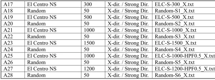
表 4.2 Benchmark A 模型的非線性試驗項目

A17 El Centro NS 300 X-dir. / Strong Dir. ELC-S-300_X.txt A18 Random 50 X-dir. / Strong Dir. Random-S1_X.txt A19 El Centro NS 500 X-dir. / Strong Dir. ELC-S-500_X.txt A20 Random 50 X-dir. / Strong Dir. Random-S2_X.txt A21 El Centro NS 1000 X-dir. / Strong Dir. ELC-S-1000_X.txt A22 Random 50 X-dir. / Strong Dir. Random-S3_X.txt A23 El Centro NS 1500 X-dir. / Strong Dir. ELC-S-1500_X.txt A24 Random 50 X-dir. / Strong Dir. Random-S4_X.txt

A25 El Centro NS 1000 X-dir. / Strong Dir. ELC-S-1000-HPF0.5_X.txt A26 Random 50 X-dir. / Strong Dir. Random-S5_X.txt

A27 El Centro NS 1200 X-dir. / Strong Dir. ELC-S-1200-HPF0.5_X.txt A28 Random 50 X-dir. / Strong Dir. Random-S6_X.txt

表 4.3 Benchmark B 模型的線性試驗項目 Test

No.

Excitation case PGA (ideal)

Direction Output File Name B1 Random 50 X-dir. / Weak Dir. Random-X-50_X.txt B2 Random 100 X-dir. / Weak Dir. Random-X-100_X.txt B3 El Centro NS 50 X-dir. / Weak Dir. ELC-X-50_X.txt B4 El Centro NS 100 X-dir. / Weak Dir. ELC-X-100_X.txt B5 ChiChi/TCU076/NS 50 X-dir. / Weak Dir. TCU076-X-50_X.txt B6 ChiChi/TCU076/NS 100 X-dir. / Weak Dir. TCU076-X-100_X.txt B7 ChiChi/TCU082/NS 50 X-dir. / Weak Dir. TCU082-X-50_X.txt B8 ChiChi/TCU082/NS 100 X-dir. / Weak Dir. TCU082-X-100_X.txt B9 Random 50 Y-dir. / Strong Dir. Random-Y-50_Y.txt B10 Random 100 Y-dir. / Strong Dir. Random-Y-100_Y.txt B11 El Centro NS 50 Y-dir. / Strong Dir. ELC-Y-50_Y.txt B12 El Centro NS 100 Y-dir. / Strong Dir. ELC-Y-100_Y.txt B13 ChiChi/TCU076/NS 50 Y-dir. / Strong Dir. TCU076-Y-50_Y.txt B14 ChiChi/TCU076/NS 100 Y-dir. / Strong Dir. TCU076-Y-100_Y.txt B15 ChiChi/TCU082/NS 50 Y-dir. / Strong Dir. TCU082-Y-50_Y.txt B16 ChiChi/TCU082/NS 100 Y-dir. / Strong Dir. TCU082-Y-100_Y.txt

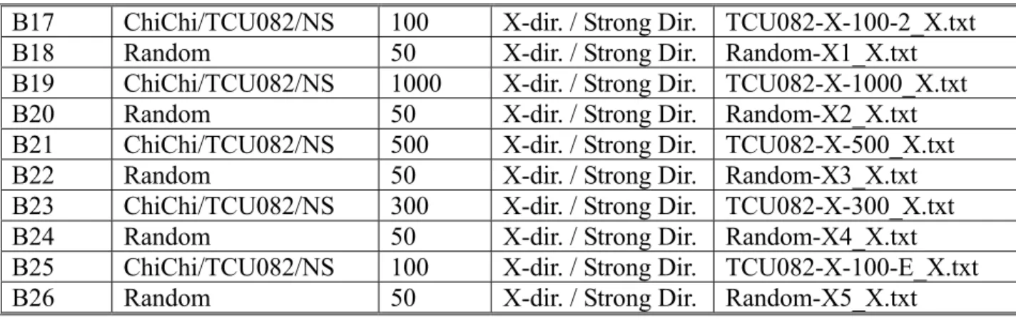
表 4.4 Benchmark B 模型的非線性試驗項目

B17 ChiChi/TCU082/NS 100 X-dir. / Strong Dir. TCU082-X-100-2_X.txt B18 Random 50 X-dir. / Strong Dir. Random-X1_X.txt B19 ChiChi/TCU082/NS 1000 X-dir. / Strong Dir. TCU082-X-1000_X.txt B20 Random 50 X-dir. / Strong Dir. Random-X2_X.txt B21 ChiChi/TCU082/NS 500 X-dir. / Strong Dir. TCU082-X-500_X.txt B22 Random 50 X-dir. / Strong Dir. Random-X3_X.txt B23 ChiChi/TCU082/NS 300 X-dir. / Strong Dir. TCU082-X-300_X.txt B24 Random 50 X-dir. / Strong Dir. Random-X4_X.txt B25 ChiChi/TCU082/NS 100 X-dir. / Strong Dir. TCU082-X-100-E_X.txt B26 Random 50 X-dir. / Strong Dir. Random-X5_X.txt

表 4.5 Benchmark C1 模型的線性試驗項目 Test

No.

Excitation case PGA (ideal)

Direction Output File Name C1 Random 50 X-dir. / Weak Dir. Random_X_50_X.txt C2 Random 100 X-dir. / Weak Dir. Random_X_100_X.txt C3 El Centro NS 50 X-dir. / Weak Dir. ELC_X_50X.txt C4 El Centro NS 100 X-dir. / Weak Dir. ELC_X100_X.txt C5 ChiChi/TCU076/NS 50 X-dir. / Weak Dir. TCU076_X_50_X.txt C6 ChiChi/TCU076/NS 100 X-dir. / Weak Dir. TCU076_X_100_X.txt C7 ChiChi/TCU082/NS 50 X-dir. / Weak Dir. TCU082_X_50_X.txt C8 ChiChi/TCU082/NS 100 X-dir. / Weak Dir. TCU082_X_100_X.txt C9 Random 50 Y-dir. / Strong Dir. Random_Y_50_Y.txt C10 Random 100 Y-dir. / Strong Dir. Random_Y_100_Y.txt C11 El Centro NS 50 Y-dir. / Strong Dir. ELC_Y_50_Y.txt C12 El Centro NS 100 Y-dir. / Strong Dir. ELC_Y_100_Y.txt C13 ChiChi/TCU076/NS 50 Y-dir. / Strong Dir. TCU076_Y_50_Y.txt C14 ChiChi/TCU076/NS 100 Y-dir. / Strong Dir. TCU076_Y_100_Y.txt C15 ChiChi/TCU082/NS 50 Y-dir. / Strong Dir. TCU082_Y_50_Y.txt C16 ChiChi/TCU082/NS 100 Y-dir. / Strong Dir. TCU082_Y_100_Y.txt

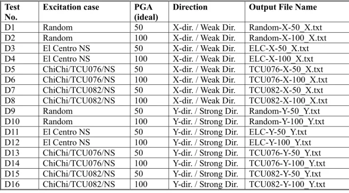
表 4.6 Benchmark D 模型（原結構）的線性試驗項目 Test

No.

Excitation case PGA (ideal)

Direction Output File Name D1 Random 50 X-dir. / Weak Dir. Random-X-50_X.txt D2 Random 100 X-dir. / Weak Dir. Random-X-100_X.txt D3 El Centro NS 50 X-dir. / Weak Dir. ELC-X-50_X.txt D4 El Centro NS 100 X-dir. / Weak Dir. ELC-X-100_X.txt D5 ChiChi/TCU076/NS 50 X-dir. / Weak Dir. TCU076-X-50_X.txt D6 ChiChi/TCU076/NS 100 X-dir. / Weak Dir. TCU076-X-100_X.txt D7 ChiChi/TCU082/NS 50 X-dir. / Weak Dir. TCU082-X-50_X.txt D8 ChiChi/TCU082/NS 100 X-dir. / Weak Dir. TCU082-X-100_X.txt D9 Random 50 Y-dir. / Strong Dir. Random-Y-50_Y.txt D10 Random 100 Y-dir. / Strong Dir. Random-Y-100_Y.txt D11 El Centro NS 50 Y-dir. / Strong Dir. ELC-Y-50_Y.txt D12 El Centro NS 100 Y-dir. / Strong Dir. ELC-Y-100_Y.txt D13 ChiChi/TCU076/NS 50 Y-dir. / Strong Dir. TCU076-Y-50_Y.txt D14 ChiChi/TCU076/NS 100 Y-dir. / Strong Dir. TCU076-Y-100_Y.txt D15 ChiChi/TCU082/NS 50 Y-dir. / Strong Dir. TCU082-Y-50_Y.txt D16 ChiChi/TCU082/NS 100 Y-dir. / Strong Dir. TCU082-Y-100_Y.txt

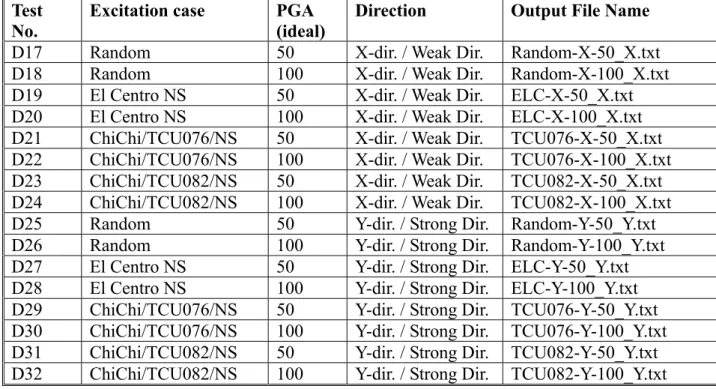
表 4.7 Benchmark D 模型（加入脆弱桿件）的線性試驗項目 Test

No.

Excitation case PGA (ideal)

Direction Output File Name D17 Random 50 X-dir. / Weak Dir. Random-X-50_X.txt D18 Random 100 X-dir. / Weak Dir. Random-X-100_X.txt D19 El Centro NS 50 X-dir. / Weak Dir. ELC-X-50_X.txt D20 El Centro NS 100 X-dir. / Weak Dir. ELC-X-100_X.txt D21 ChiChi/TCU076/NS 50 X-dir. / Weak Dir. TCU076-X-50_X.txt D22 ChiChi/TCU076/NS 100 X-dir. / Weak Dir. TCU076-X-100_X.txt D23 ChiChi/TCU082/NS 50 X-dir. / Weak Dir. TCU082-X-50_X.txt D24 ChiChi/TCU082/NS 100 X-dir. / Weak Dir. TCU082-X-100_X.txt D25 Random 50 Y-dir. / Strong Dir. Random-Y-50_Y.txt D26 Random 100 Y-dir. / Strong Dir. Random-Y-100_Y.txt D27 El Centro NS 50 Y-dir. / Strong Dir. ELC-Y-50_Y.txt D28 El Centro NS 100 Y-dir. / Strong Dir. ELC-Y-100_Y.txt D29 ChiChi/TCU076/NS 50 Y-dir. / Strong Dir. TCU076-Y-50_Y.txt D30 ChiChi/TCU076/NS 100 Y-dir. / Strong Dir. TCU076-Y-100_Y.txt D31 ChiChi/TCU082/NS 50 Y-dir. / Strong Dir. TCU082-Y-50_Y.txt D32 ChiChi/TCU082/NS 100 Y-dir. / Strong Dir. TCU082-Y-100_Y.txt

表 4.8 Benchmark D 模型（加入脆弱桿件）的非線性試驗項目

D33 ChiChi/TCU082/NS 100 X-dir. / Strong Dir. TCU082-X-100-2_X.txt D34 Random 50 X-dir. / Strong Dir. Random-X1_X.txt D35 ChiChi/TCU082/NS 1000 X-dir. / Strong Dir. TCU082-X-1000_X.txt D36 Random 50 X-dir. / Strong Dir. Random-X2_X.txt D37 ChiChi/TCU082/NS 500 X-dir. / Strong Dir. TCU082-X-500_X.txt D38 Random 50 X-dir. / Strong Dir. Random-X3_X.txt D39 ChiChi/TCU082/NS 300 X-dir. / Strong Dir. TCU082-X-300_X.txt D40 Random 50 X-dir. / Strong Dir. Random-X4_X.txt D41 ChiChi/TCU082/NS 100 X-dir. / Strong Dir. TCU082-X-100-E_X.txt D42 Random 50 X-dir. / Strong Dir. Random-X5_X.txt Note: Nonlinear test (with weak element at the bottom of 1F)

表 4.9 Benchmark A 經類神經網路分析所得之頻率和阻尼（線性，震動方向為 X 向） 試驗編號 阻尼頻率 阻尼比 自然頻率 備註 8.0577 0.0019 8.0578 6.4015 0.0305 6.4045 實際上不存在 4.5022 0.0018 4.5022 A1 1.3480 0.0181 1.3482 8.0560 0.0019 8.0560 6.4464 0.0144 6.4470 實際上不存在 4.5006 0.0018 4.5006 A2 1.3458 0.0193 1.3461 8.0574 0.0018 8.0574 6.3960 0.0067 6.3961 實際上不存在 4.5016 0.0018 4.5016 A5 1.3498 0.0238 1.3502 8.0533 0.0019 8.0533 6.3755 0.0044 6.3756 實際上不存在 4.4967 0.0017 4.4967 1.3466 0.0243 1.3470 A6 2.0646 0.0339 2.0658 實際上不存在 8.0532 0.0019 8.0532 6.3736 0.0136 6.3741 實際上不存在 4.4994 0.0019 4.4994 A7 1.3420 0.0225 1.3424 8.0474 0.0023 8.0474 6.2695 0.0063 6.2696 實際上不存在 4.4917 0.0024 4.4917 A8 1.3330 0.0242 1.3334

表 4.10 Benchmark A 經類神經網路分析所得之頻率和阻尼（線性，震動方向為 Y 向） 試驗編號 阻尼頻率 阻尼比 自然頻率 備註 A9 6.4219 0.0164 6.4227 實際上不存在 5.1420 0.0018 5.1420 3.3040 0.0018 3.3040 A10 1.0806 0.0155 1.0807 5.1406 0.0024 5.1406 3.3025 0.0019 3.3025 A13 1.0871 0.0251 1.0874 5.1387 0.0023 5.1387 3.2990 0.0021 3.2990 A14 1.0783 0.0200 1.0785 6.4121 0.0010 6.4121 實際上不存在 5.1419 0.0019 5.1419 3.3035 0.0019 3.3036 A15 1.0852 0.0197 1.0854 6.3868 0.0042 6.3868 實際上不存在 5.1389 0.0018 5.1389 3.3001 0.0019 3.3001 A16 1.0786 0.0177 1.0787

表 4.11 Benchmark A 經類神經網路分析所得之頻率和阻尼（非線性，震動方向為 X 向） 試驗編號 阻尼頻率 阻尼比 自然頻率 備註 8.0477 0.0019 8.0477 4.4911 0.0022 4.4911 A18 1.3420 0.0192 1.3422 1.3383 0.0195 1.3386 4.4851 0.0023 4.4851 A20 8.0415 0.0022 8.0415 1.3316 0.0194 1.3319 4.4745 0.0025 4.4745 8.0341 0.0021 8.0341 A22 6.2660 0.0322 6.2693 實際上不存在 8.0339 0.0022 8.0339 6.3978 0.0364 6.4020 實際上不存在 4.4750 0.0024 4.4750 A24 1.3304 0.0206 1.3306 8.0312 0.0021 8.0313 6.4265 0.0428 6.4324 實際上不存在 4.4725 0.0023 4.4725 A26 1.3293 0.0194 1.3296 8.0282 0.0022 8.0283 6.5218 0.0307 6.5249 實際上不存在 4.4700 0.0022 4.4700 A28 1.3277 0.0190 1.3279

表 4.12 Benchmark B 經類神經網路分析所得之頻率和阻尼（非線性，震動方向為 X 向） 試驗編號 阻尼頻率 阻尼比 自然頻率 備註 7.2910 0.0398 7.2967 實際上不存在 5.1167 0.0016 5.1167 3.2631 0.0016 3.2631 B1 1.0853 0.0336 1.0859 5.1112 0.0017 5.1112 3.2585 0.0018 3.2585 B2 1.0826 0.0328 1.0831 5.1175 0.0014 5.1175 3.2622 0.0015 3.2622 B5 1.0735 0.0242 1.0738 5.1146 0.0016 5.1146 3.2592 0.0017 3.2592 B6 1.0698 0.0223 1.0701 5.1158 0.0015 5.1158 3.2604 0.0015 3.2604 B7 1.0709 0.0220 1.0712 5.1150 0.0015 5.1150 3.2592 0.0016 3.2592 B8 1.0700 0.0234 1.0703

表 4.13 Benchmark B 經類神經網路分析所得之頻率和阻尼（線性，震動方向為 Y 向） 試驗編號 阻尼頻率 阻尼比 自然頻率 備註 8.1704 0.0017 8.1704 7.4651 0.0088 7.4654 實際上不存在 4.6779 0.0017 4.6780 B10 1.3975 0.0192 1.3977 8.1683 0.0017 8.1683 7.3932 0.0018 7.3932 4.6755 0.0016 4.6755 B13 1.3950 0.0177 1.3952 8.1602 0.0017 8.1602 7.4293 0.0016 7.4293 4.6689 0.0018 4.6689 B14 1.3887 0.0184 1.3890 8.1685 0.0018 8.1686 7.4446 0.0008 7.4446 4.6766 0.0015 4.6766 B15 1.3913 0.0186 1.3915 8.1595 0.0019 8.1595 7.4320 0.0021 7.4320 4.6691 0.0018 4.6691 B16 1.3862 0.0188 1.3865

表 4.14 Benchmark B 經類神經網路分析所得之頻率和阻尼（非線性，震動方向為 X 向） 試驗編號 阻尼頻率 阻尼比 自然頻率 備註 7.2231 0.0249 7.2253 實際上不存在 5.1122 0.0017 5.1122 3.2572 0.0019 3.2572 B17 1.0715 0.0192 1.0717 7.4264 0.0082 7.4267 實際上不存在 5.1155 0.0015 5.1155 1.0734 0.0207 1.0737 B18 3.2602 0.0016 3.2602 7.4388 0.0060 7.4389 實際上不存在 5.1093 0.0014 5.1093 1.0611 0.0213 1.0613 2.3377 0.0295 2.3387 B20 3.2473 0.0016 3.2473 7.4401 0.0049 7.4402 實際上不存在 5.1092 0.0015 5.1092 2.3364 0.0348 2.3378 1.0598 0.0199 1.0600 B22 3.2466 0.0016 3.2466 7.4390 0.0054 7.4391 實際上不存在 5.1091 0.0014 5.1091 3.2462 0.0016 3.2462 2.3364 0.0402 2.3383 B24 1.0600 0.0199 1.0602 7.4489 0.0042 7.4490 實際上不存在 5.1092 0.0014 5.1092 1.0603 0.0196 1.0605 2.3474 0.0421 2.3495 B26 3.2464 0.0016 3.2464

表 4.15 Benchmark C1 經類神經網路分析所得之頻率和阻尼（線性，震動方向為 X 向） 試驗編號 阻尼頻率 阻尼比 自然頻率 備註 5.1411 0.0018 5.1411 3.2679 0.0020 3.2679 C1 1.0769 0.0227 1.0772 5.1379 0.0017 5.1379 3.2647 0.0020 3.2647 C2 1.0744 0.0205 1.0747 5.1366 0.0017 5.1366 3.2627 0.0020 3.2627 C5 1.0719 0.0197 1.0721 7.2969 0.0310 7.3004 實際上不存在 5.1341 0.0018 5.1341 3.2586 0.0021 3.2586 2.3171 0.0078 2.3172 C6 1.0669 0.0192 1.0671 7.3161 0.0201 7.3176 實際上不存在 5.1359 0.0017 5.1359 3.2624 0.0019 3.2624 C7 1.0725 0.0210 1.0727 7.2599 0.0152 7.2608 實際上不存在 5.1325 0.0018 5.1325 3.2591 0.0019 3.2591 2.3002 0.0392 2.3019 C8 1.0677 0.0204 1.0679

表 4.16 Benchmark C1 經類神經網路分析所得之頻率和阻尼（線性，震動方向為 Y 向） 試驗編號 阻尼頻率 阻尼比 自然頻率 備註 8.2122 0.0019 8.2122 7.3592 0.0082 7.3594 4.6607 0.0019 4.6607 2.3696 0.0366 2.3712 C10 1.4038 0.0187 1.4041 8.2082 0.0020 8.2082 7.3695 0.0047 7.3696 4.6569 0.0020 4.6569 C13 1.3984 0.0180 1.3986 8.2008 0.0020 8.2008 7.3284 0.0085 7.3287 4.6487 0.0021 4.6487 1.3914 0.0175 1.3916 C14 2.3854 0.0235 2.3860 8.2035 0.0019 8.2035 7.3468 0.0043 7.3469 4.6510 0.0017 4.6510 C15 1.3935 0.0170 1.3937 8.1914 0.0017 8.1915 7.3315 0.0054 7.3316 4.6389 0.0022 4.6389 2.5540 0.0472 2.5568 C16 1.3868 0.0179 1.3870

表 4.17 Benchmark D 經類神經網路分析所得之頻率和阻尼（D1~D8） 試驗編號 阻尼頻率 阻尼比 自然頻率 備註 7.3444 0.0116 7.3449 實際上不存在 5.1227 0.0013 5.1227 3.2444 0.0016 3.2444 D1 1.0575 0.0168 1.0576 1.0571 0.0166 1.0572 2.2892 0.0121 2.2894 3.2425 0.0015 3.2425 5.1207 0.0015 5.1207 D2 7.2227 0.0367 7.2276 實際上不存在 7.2907 0.0098 7.2911 實際上不存在 5.1184 0.0016 5.1184 3.2389 0.0016 3.2389 1.0573 0.0182 1.0575 D5 2.2709 0.0341 2.2723 實際上不存在 7.3554 0.0220 7.3572 實際上不存在 5.1150 0.0019 5.1151 3.2346 0.0018 3.2346 2.2597 0.0147 2.2600 D6 1.0568 0.0220 1.0570 7.3278 0.0153 7.3286 實際上不存在 5.1168 0.0016 5.1168 3.2371 0.0018 3.2371 2.2590 0.0342 2.2603 D7 1.0568 0.0164 1.0569 7.2599 0.0152 7.2608 實際上不存在 5.1325 0.0018 5.1325 3.2591 0.0019 3.2591 2.3002 0.0392 2.3019 D8 1.0677 0.0204 1.0679

表 4.18 Benchmark D 經類神經網路分析所得之頻率和阻尼（D9~D16） 試驗編號 阻尼頻率 阻尼比 自然頻率 備註 8.1407 0.0016 8.1407 7.3211 0.0080 7.3213 4.6137 0.0017 4.6137 D10 1.3807 0.0181 1.3809 1.3710 0.0166 1.3712 4.6030 0.0016 4.6030 7.2574 0.0091 7.2577 D13 8.1316 0.0018 8.1316 8.1244 0.0022 8.1244 7.1938 0.0119 7.1943 4.5979 0.0020 4.5979 2.2755 0.0119 2.2756 D14 1.3660 0.0164 1.3662 8.1263 0.0024 8.1263 7.3195 0.0007 7.3195 4.6004 0.0017 4.6004 2.2782 0.0098 2.2783 D15 1.3686 0.0145 1.3688 8.1138 0.0025 8.1138 7.3100 0.0016 7.3100 4.5896 0.0025 4.5897 2.2846 0.0018 2.2846 D16 1.3622 0.0139 1.3623

表 4.19 Benchmark D 經類神經網路分析所得之頻率和阻尼（D17~D24） 試驗編號 阻尼頻率 阻尼比 自然頻率 備註 7.1774 0.0108 7.1779 5.0832 0.0016 5.0832 3.1783 0.0018 3.1784 D18 1.0272 0.0273 1.0276 7.2643 0.0111 7.2648 實際上不存在 5.0859 0.0015 5.0859 3.1804 0.0015 3.1804 1.0293 0.0209 1.0295 D21 2.2835 0.0383 2.2852 7.2949 0.0261 7.2974 實際上不存在 5.0821 0.0019 5.0821 3.1760 0.0019 3.1760 2.2612 0.0103 2.2613 D22 1.0271 0.0172 1.0272 7.2446 0.0119 7.2451 實際上不存在 5.0837 0.0015 5.0837 3.1789 0.0017 3.1789 D23 1.0295 0.0195 1.0297 5.0808 0.0018 5.0808 3.1752 0.0021 3.1752 2.3570 0.0383 2.3587 D24 1.0336 0.0211 1.0338

表 4.20 Benchmark D 經類神經網路分析所得之頻率和阻尼（D25~D32） 試驗編號 阻尼頻率 阻尼比 自然頻率 備註 7.6515 0.0275 7.6544 D25* 3.8146 0.0622 3.8220 7.6385 0.0213 7.6402 D26* 3.9347 0.0568 3.9411 7.3104 0.0109 7.3109 4.2770 0.0311 4.2790 D29* 2.5269 0.0997 2.5395 7.2541 0.0141 7.2548 4.1514 0.0323 4.1536 D30* 2.3520 0.0251 2.3528 7.3145 0.0008 7.3145 實際上不存在 5.1809 0.0220 5.1822 3.5150 0.0372 3.5175 D31* 2.3200 0.0425 2.3221 7.3075 0.0008 7.3075 5.1988 0.0246 5.2004 3.4413 0.0238 3.4423 D32* 2.3075 0.0222 2.3080 註：* 表示尚有一些頻率未被分析出來。

表 4.21 Benchmark D 經類神經網路分析所得之頻率和阻尼（D33~D42） 試驗編號 阻尼頻率 阻尼比 自然頻率 備註 7.2666 0.0037 7.2666 實際上不存在 5.0776 0.0020 5.0776 3.1671 0.0027 3.1671 2.1677 0.0102 2.1678 D33 1.0227 0.0134 1.0228 7.1606 0.0087 7.1609 4.9647 0.0059 4.9648 2.9765 0.0333 2.9781 D35* 2.2472 0.0773 2.2539 7.0769 0.0132 7.0775 實際上不存在 5.0239 0.0021 5.0239 3.0616 0.0183 3.0621 D37* 2.3657 0.0449 2.3681 7.2344 0.0026 7.2344 5.0595 0.0021 5.0595 3.1088 0.0100 3.1089 2.2700 0.0299 2.2710 D39 0.9889 0.0365 0.9895 7.2533 0.0016 7.2533 實際上不存在 5.0641 0.0030 5.0642 3.1554 0.0027 3.1554 2.2530 0.0156 2.2533 D41 1.0061 0.0224 1.0064 註：* 表示尚有一些頻率未被分析出來。

1 圖 2.1、典型之三層類神經網路架構圖 2 2 2 1 1 Ni Nh No i j k 隱藏層 y1 x1 輸入層 輸出層 x2 xNi y2 yNo vjk wij xk yi

圖 3.1、類神經網路系統識別模式之網路架構圖 ) 1 ( 2 t− x&& ) 1 (t− x&&k ) 1 ( 1 t− x&& ) ( 2 t m x&& − ) (t m x&&_k − ) ( 1 t m x&& − ) ( 2 t n f − ) (t n f_l − ) ( 1 t n f − ) ( 1 t x&& ) ( 2 t x&& ) ( 3 t x&& ) ( 1 t f ) ( 2 t f ) ( 4 t x&& ) (t f_l 輸入層 ) (t x&&k 輸出層 隱藏層

Benchmark A, B, C1 &

D

Benchmark C2

Benchmark C3

Benchmark C4