應用基於消失點之影像校正於強健式人臉偵測

(1)

國

立

交

通

大

學

多媒體工程研究所

碩

士

論

文

應用基於消失點之影像校正於強健式人臉偵測

Vanishing Point-Based Image Rectification for Robust Face Detection

研究生：王靖賀

指導教授：莊仁輝教授

(2)

應用基於消失點之影像校正於強健式人臉偵測

Vanishing Point-Based Image Rectification for Robust Face Detection

研究生：王靖賀 Student：Ching-Ho Wang

指導教授：莊仁輝 Advisor：Jen-Hui Chuang

國立交通大學

多媒體工程研究所

碩士論文

A Thesis

Submitted to Institute of MultimediaEngineering

College of Computer Science

National Chiao Tung University

in partial Fulfillment of the Requirements

for the Degree of

Master

in

Computer Science

July 2013

Hsinchu, Taiwan, Republic of China

(3)

i

應用基於消失點之影像校正

於強健式人臉偵測

學生：王靖賀指導教授：莊仁輝博士

國立交通大學

多媒體工程研究所碩士班

摘要

我們提出一種新的基於消失點影像校正方法以提高一般監控式系統性能，雖然大多數現有的人臉資料庫和偵測技術都是基於相機和人臉在同個高度上的假設，但在實際狀況下，相機很有可能會被安裝在不同的高度上，因此這種差異通常會降低基於正面人臉影像學習演算法的效能。在這篇論文當中，我們提出影像轉換來校正人臉影像，因此在訓練過程中可以不必蒐集不同的人臉方向。此外為了達到更佳的偵測效果，我們還提出基於膚色分析來降低錯誤偵測的方法。在實驗結果中表明我們所提出的方法在人臉偵測中可以得到顯著的改善。

(4)

ii

Vanishing Point-Based Image Rectification for Robust Face Detection

Student：Ching-Ho Wang Advisor：Dr. Jen-Hui Chuang

Institute of Multimedia Engineering

National Chiao Tung University

Abstract

We proposed a novel face detection method based on the vanishing point of vertical lines

image rectification to improve system performance in a common surveillance application.

While most existing face datasets and detection techniques are based on the assumption that

the camera has a similar height as the target faces, in practical situations the camera may be

installed at different heights. Such discrepancy often degrades the detection performance of

algorithms based on learning with frontal face orientation. In this thesis we propose a

transformation to rectify face images such that it is not necessary to collect training data of

different face orientations. Furthermore, a method for reducing false alarms by skin analysis is

proposed for better performance. The experiments show prominent improvements in face

(5)

iii

Acknowledgement

I would like to express my great appreciation to Dr. Jen-Hui Chung, for his patient

guidance, enthusiastic encouragement and useful suggestions of this thesis. His willingness to

give his time so generously has been very much appreciated. I also appreciate my thesis

committees, Dr. Hsu-Chun Yen, Dr. Chin-Laung Lei and Dr. Tsai-Pei Wang. Because of their

helpful advices make me to complete this thesis more easily.

In addition, I would like to take this opportunity to thank to the helps provided by all the

members of the Intelligent System Laboratory at National Chiao Tung University during the

planning and development of this research work. Finally, I would also thank for my parents

(6)

iv

List of Figures

FIGURE 1.1:EXAMPLE OF A PERSON WALKING TOWARD A CAMERA WITH ORDINARY FORWARD-LOOKING FACE IN DIFFERENT DIRECTION.(A)A PERSON WALKS TOWARD THE CAMERA IN A STRAIGHT PATH.(B)A

PERSON WALKS TOWARD THE CAMERA IN A DIFFERENT PATH IN (A). ... 2

FIGURE 1.2:(A)ORIGINAL FRONTAL FACE.(B)A BILLBOARD WITH PATTERNS REPRESENTING (A).(C)IMAGE CAPTURED BY SURVEILLANCE CAMERA AT A HIGHER-UP LOCATION.(D)A BILLBOARD WITH PATTERNS REPRESENTING (C). ... 2

FIGURE 1.3:AN IMAGE WITH THREE CHESSBOARDS WITH DIFFERENT POSITIONS CAPTURED BY A HIGHER-UP POSITION CAMERA. ... 3

FIGURE 1.4:DIFFERENT STRUCTURE OF MVFD.(A)PARALLEL CASCADES.(B)WFSTREE. ... 4

FIGURE 1.5:FLOWCHART OF THE PROPOSE FACE DETECTION APPROACH. ... 6

FIGURE 2.1:RECTIFICATION RESULTS OF FIGURES 1.2(C) AND (D).(A)-(B)OBTAINED FROM TRANSFORMATION 1 DISCUSSED IN SECTION 2.1.(C)-(D)OBTAINED FROM TRANSFORMATION 2 DISCUSSED IN SECTION 2.2. ... 7

FIGURE 2.2:THE RELATION BETWEEN THE CAMERA, A STANDING BILLBOARD, AND THE GROUND PLANE, WITH THE CAMERA REPRESENTED BY ITS LENS FOR SIMPLICITY.THE BILLBOARD IS ASSUMED TO BE FACING THE VERTICAL LINE CONTAINING THE CAMERA CENTER. ... 8

FIGURE 2.3:AN ILLUSTRATION DIAGRAM FOR TRANSFORM 1.(A)IMAGE BEFORE RECTIFIED.(B)IMAGE AFTER RECTIFIED. ... 10

FIGURE 2.4:(A)ORIGIN IMAGE.(B)RECTIFIED RESULT OF TRANSFORMATION 1. ... 10

FIGURE 2.5:A ROTATION OF FIGURE 2.2, TO MAKE THE OPTICAL AXIS OF THE CAMERA HORIZONTAL. ... 11

FIGURE 2.6:AN ILLUSTRATION SHOWING THE RELATIONSHIP BETWEEN THE IMAGE SENSOR AND THE IMAGE. ... 12

FIGURE 2.8:RECTIFIED IMAGE OF FIGURE 1.1(B) BY TRANSFORMATION 2 AND 3.(A)RESULT OF TRANSFORMATION 2.(B)RESULT OF TRANSFORMATION 3. ... 14

FIGURE 2.9:RELATION BETWEEN ORIGINAL IMAGE AND RECTIFIED IMAGE BY TRANSFORMATION 3.(A)ORIGINAL IMAGE.(B)RECTIFIED IMAGE BY TRANSFORMATION 3. ... 15

FIGURE 3.1:SKIN COLOR REGION DEFINE BY [16] AT Y=110 AND Y=140.(A)YCBCR PLANE AT DIFFERENT Y VALUE.(B)SKIN REGION DEFINE BY EQUATION 3.1.(C)SKIN COLORS AT DIFFERENT Y VALUE. ... 18

FIGURE 3.2:(A)A PICTURE WITH FIVE CANDIDATE REGIONS.(B)0% SKIN COLOR PERCENTAGE IN REGION 1.(C) 33% SKIN COLOR PERCENTAGE IN REGION 2.(D)0% SKIN COLOR PERCENTAGE IN REGION 3.(E)79% SKIN COLOR PERCENTAGE IN REGION 4.(F)0% SKIN COLOR PERCENTAGE IN REGION 5. ... 19

FIGURE 3.3:VIDEOS USED TO FIND THE THRESHOLD OF SKIN PIXEL PERCENTAGE.(A)VIDEO S10.(B)VIDEO O5. 20 FIGURE 3.4:REDUCING FALSE ALARMS WITH 40% SKIN COLOR IN CANDIDATE REGIONS METHOD IN DIFFERENT PATH IMAGES. ... 23

(8)

vi

FIGURE 4.1:CAMERA AXIS207MW SETTINGS.(A)EXPERIMENTAL ENVIRONMENT.(B)CLOSE-UP VIEW OF CAMERA. ... 25

FIGURE 4.2:CAMERA VIVOTEKFD8161 SETTINGS.(A)EXPERIMENTAL ENVIRONMENT.(B)CLOSE-UP VIEW OF CAMERA. ... 25

FIGURE 4.3:FRAME EXAMPLES OF A SINGLE PERSON WALKING IN THE LABORATORY.(A)VIDEO S1.(B)VIDEO S2. (C)VIDEO S3.(D)VIDEO S4.(E)VIDEO S5.(F)VIDEO S6.(G)VIDEO S7.(H)VIDEO S8.(I)VIDEO S9. (J)VIDEO S10. ... 26

FIGURE 4.4:FRAME EXAMPLES OF MULTI PEOPLE WALKING IN THE LABORATORY.(A)VIDEO M1.(B)VIDEO M2.(C) VIDEO M3.(D)VIDEO M4.(E)VIDEO M5.(F)VIDEO M6.(G)VIDEO M7. ... 27

FIGURE 4.5:FRAME EXAMPLES OF A SINGLE PERSON WALKING IN THE OUTDOOR ENVIRONMENT.(A)VIDEO O1.(B) VIDEO O2.(C)VIDEO O3.(D)VIDEO O4.(E)VIDEO O5.(F)VIDEO O6.(G)VIDEO O7.(H)VIDEO O8. ... 27 FIGURE 4.6:THE RELATIONSHIP BETWEEN FIVE CAMERAS AND HUMAN FACE IN MUCT. ... 28

FIGURE 4.7:THREE DIFFERENT LIGHTING FOR A PERSON IN MUCT FACE DATABASE CAPTURED BY CAMERA E. .... 29

FIGURE 4.8:THE TESTING RESULT OF FIGURE 4.7(A).1=FACE WAS DETECTED;0=NO FACE WAS DETECTED.

22-(-25)+1=48,48 IS THE MAXIMUM ROTATION IN PLANE DEGREE RESULT FOR FIGURE 4.7(A). ... 29

FIGURE 4.9:EXAMPLE OF ROTATING IMAGE.(A)ORIGIN IMAGE.(B)ROTATE -15 DEGREE.(C)ROTATE 15 DEGREE. (D)ROTATE -30 DEGREE.(E)ROTATE 30 DEGREE. ... 30

FIGURE 4.10:COMBINE THE DETECTION RESULTS OF FIGURE 4.9 INTO ONE IMAGE.(A)COMBINE FIGURE 4.9(A)-(C)

AND 2TP/FP IN THE IMAGE.(B)COMBINE FIGURE 4.9(A)-(E) AND 3TP/FP IN THE IMAGE. ... 30

FIGURE 4.11:RESULTS OF S3 VIDEO.(A)RESULTS OF O.(B)RESULTS OF T1.(C)RESULTS OF T2.(D)RESULT OF

T3. ... 33 FIGURE 4.12:RESULTS OF M7 VIDEO.(A)RESULTS OF O.(B)RESULTS OF T1.(C)RESULTS OF T2.(D)RESULT OF

T3. ... 35 FIGURE 4.13:RESULTS OF O8 VIDEO.(A)RESULTS OF O.(B)RESULTS OF T1.(C)RESULTS OF T2.(D)RESULT OF

T3. ... 36 FIGURE 4.14:THE ENVIRONMENT OF SYNTHETIC SCENE.(A)AN AERIAL IMAGE OF THE SYNTHETIC SCENE.(B)A

SIDE VIEW OF THE SYNTHETIC SCENE WITH CAMERA AT 3 METERS HEIGHT AND 40 DEGREE ANGLE OF DEPRESSION. ... 41

FIGURE 4.15:EXAMPLES OF SYNTHETIZED IMAGES CAPTURE BY CAMERA.(A)2M, .(B)4M, . ... 41 FIGURE 4.16:THE DETECTION RATES OF DIFFERENT TRANSFORMATIONS BY DIFFERENT CAMERA SETTINGS.(A)THE DETECTION RATES FROM DIFFERENT TRANSFORMATIONS ACCORDING TO VARYING CAMERA HEIGHTS. (B)THE DETECTION RATES FROM DIFFERENT TRANSFORMATIONS ACCORDING TO VARYING CAMERA ANGLES... 42

FIGURE 4.17:THE DETECTION RATES OF DIFFERENT FACE DETECTION METHODS BY DIFFERENT CAMERA SETTINGS. (A)THE DETECTION RATES FROM DIFFERENT FACE DETECTION METHODS ACCORDING TO VARYING CAMERA HEIGHTS.(B)THE DETECTION RATES FROM DIFFERENT FACE DETECTION METHODS

(9)

vii

List of Tables

TABLE 3.1:THE DETECTION RESULTS FOR S10 WITH DIFFERENT THRESHOLDS OF SKIN PIXEL PERCENTAGE. ... 21

TABLE 3.2:THE DETECTION RESULTS FOR O5 WITH DIFFERENT THRESHOLDS OF SKIN PIXEL PERCENTAGE. ... 22

TABLE 4.1:FACE DETECTION RESULTS OF S1~S10 VIDEOS BY IMAGE ROTATION. ... 31

TABLE 4.2:FACE DETECTION RESULTS OF M1~M7 VIDEOS BY IMAGE ROTATION. ... 32

TABLE 4.3:FACE DETECTION RESULTS OF O1~O8 VIDEOS BY IMAGE ROTATION. ... 32

TABLE 4.4:AVERAGE DETECTION RESULTS OF IMAGE ROTATION METHOD. ... 33

TABLE 4.5:FACE DETECTION RESULTS OF S1~S10 VIDEOS BY IMAGE RECTIFICATION. ... 34

TABLE 4.6:FACE DETECTION RESULTS OF M1~M7 VIDEOS BY IMAGE RECTIFICATION. ... 35

TABLE 4.7:FACE DETECTION RESULTS OF O1~O8 VIDEOS BY IMAGE RECTIFICATION. ... 36

TABLE 4.8:AVERAGE DETECTION RESULTS OF IMAGE RECTIFICATION METHOD. ... 37

TABLE 4.9:THE COMPUTATION TIME(S) OF EACH FACE DETECTION METHODS. ... 37

TABLE 4.10:FACE DETECTION RESULTS OF S1~S10 VIDEOS BY IMAGE RECTIFICATION WITH REDUCING FALSE ALARMS. ... 38

TABLE 4.11:FACE DETECTION RESULTS OF M1~M7 VIDEOS BY IMAGE RECTIFICATION WITH REDUCING FALSE ALARMS. ... 39

TABLE 4.12:FACE DETECTION RESULTS OF O1~O8 VIDEOS BY IMAGE RECTIFICATION WITH REDUCING FALSE ALARMS. ... 39

TABLE 4.13:AVERAGE DETECTION RESULTS OF IMAGE RECTIFICATION WITH REDUCING FALSE ALARMS. ... 40

(10)

1

Chapter 1 Introduction

1.1 Motivation

In recent years, computer vision techniques are widely used in the world, such as

surveillance systems [1], access control systems [2] and computer login systems [3]. Most

face detection approaches are based on supervised machine learning and highly depend on the

training data used in the learning stage. To achieve good performance in the detection,

training data under various environmental factors are often needed. However, since it is hard

to always collect sufficient training data for so many factors, many researchers try to lessen

the effects of these factors. While some researchers focus on developing more robust features

or representations [4], others try to recover the underlying properties of the entire image [5] or

the target of interest [6].

In this thesis, alleviation of the effect of perspective distortion introduced by a security

camera mounted at a higher position, which is usually encountered in common surveillance

applications, is considered for face detection. Although most face datasets do include

variations such as different lightings, occlusions, and poses, we focus on such an application

since most researches on face detection are devoted to the special case that all faces are

assumed to have about the same height as the camera. Specifically, we aim to improve face

detection performance under this practical condition wherein the camera is installed at a

position higher than the human head to avoid any tampering. For example, the camera may be

installed above an entrance through which people are entering from different directions with

the ordinary forward-looking face orientation, as shown in Figure 1.1. With such setting, the

inconstancy between the captured faces and those faces in a training set is illustrated in Figure

(11)

2

inconstancy. Moreover, the camera is assumed to be mounted casually, only adjusted for

proper viewing angle for surveillance purpose, while its exact location and orientation are

actually unmeasured. The only required information for the proposed face detection approach

is the vanishing point of vertical lines (VPVL), which can be obtained easily. Under such

conditions, we propose three image transformations based on VPVL to partially correct the

perspective distortion to improve the performance of face detection for common surveillance

camera configuration.

(a) (b)

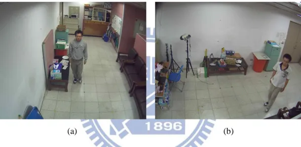
Figure 1.1: Example of a person walking toward a camera with ordinary forward-looking face in different direction. (a) A person walks toward the camera in a straight path. (b) A person walks toward the camera in a different path in (a).

(a) (b) (c) (d)

Figure 1.2: (a) Original frontal face. (b) A billboard with patterns representing (a). (c) Image captured by surveillance camera at a higher-up location. (d) A billboard with patterns representing (c).

(12)

3

1.2 Related Work

Image rectification and face detection have both been studied for a long period of time

and numerous techniques have been developed. In the following two subsections we briefly

introduce some most related work.

1.2.1 Image Rectification

Image rectification is a widely investigated topic. Much of the prior work use different

calibration methods to estimate camera parameters and the geometric relation between the 2D

image and the 3D scene. In fact, research on this problem is rather mature if sufficient

auxiliary tools and manually given marks are used. Often, special objects with specific shapes

or patterns are needed for developing the transformation for image rectification. From a

different point of view, other methods exploit the structure presented in the image to ease the

calibration process. The most straightforward approaches for image rectification are to detect

multiple vanishing points (two for each planar patch) [7-12], by edge detection and voting,

texture analysis, etc. One major assumption of these approaches is that the content in the

image is sufficient enough so that the aforementioned vanishing points can be estimated

correctly. For example, Figure 1.3 shows three vertical chessboards with different orientations

that four vanishing points can be obtained from their black/white edges. Different from all the

existing approaches, three image rectification methods based on a single vanishing point are

proposed for enhancement of face detection in this thesis and will be detailed in chapter 2.

(13)

4

1.2.2 Face Detection Techniques

Face detection is also a popular topic with plentiful literatures. Among them the

remarkable work proposed by Viola and Jones [13] attracts vast attention in recent years.

There are three main contributions in [13] first, the integral image is used to efficiently

compute a rich set of image features; second, the learning algorithm, Adaboost, is used to

enhance the result of face detection; third, a cascade of several weak classifiers is proposed to

reduce computation time and improve detection accuracy.

(a) (b)

Figure 1.4: Different structure of MVFD. (a) Parallel Cascades. (b) WFS Tree.

The efficiency and effectiveness of [13] make it a basis of the other two related

multi-view face detection (MVFD) works [14, 15]. While in [13] the system is intended for

detecting frontal faces only, in [14] and [15] faces with rotations up to ±90-degree

rotation-out-of-plane and 360-degree rotation-in-plane are also detected. In most MVFD

literatures, human faces are divided into different categories according to the variant

appearances from different view points. The authors in [14] configure weak classifiers as

confidence-rated look-up table of Haar feature for each view category and use Real Adaboost

algorithm to boost them. Furthermore, they also use a nesting-structured detector with a

(14)

5

most MVFD methods, the cascades are trained individually for each view, as shown in Figure

1.4(a). Therefore the complexity of computation makes it hard to reach real-time performance.

In [15], a real-time MVFD method with a carefully designed cascade structure, named

Width-First-Search (WFS) tree structure, is proposed. WFS adopts the coarse-to-fine strategy

which divides entire face space into smaller subspaces, as shown in Figure 1.4(b). Although it

improves computational efficiency and accuracy, it is still hard to get satisfied detection

performance when it comes to the application we discussed in this thesis, i.e., face detection

with a surveillance camera mounted at a higher-up location.

1.3 Organization of thesis

In this thesis we propose a novel image transform based on the vanishing point of

vertical lines in the scene to improve the performance of face detection for a surveillance

camera with a common higher up mounting position. The flowchart of the proposed face

detection approach in this thesis is shown in Figure 1.5. For each video frame, we first solve

the image distortion problem with one of the proposed image transformations and then use the

face detectors to get face candidates in the transformed image. To further reduce false alarms,

we also propose to use skin color analysis to remove some candidates reported by the face

detectors.

The rest of this thesis is organized as follows. In Chapter 2, we detail the image

transform approach. In Chapter 3, we use skin color percentage in the detection window to

reduce false alarms. The experimental results are shown in Chapter 4 and one can see the

proposed methods can significantly enhance the detection performance. Finally, we give

(15)

6

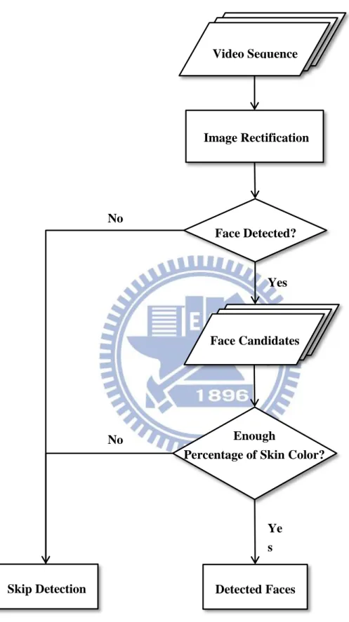
Figure 1.5: Flowchart of the propose face detection approach.

Enough

Percentage of Skin Color?

Face Candidates Face Detected? Image Rectification Video Sequence Detected Faces Skip Detection Yes No Ye s No

(16)

7

Chapter 2 Vanishing Point-based Image Rectification

In this chapter we present three different yet related transformations to rectify images

having the perspective distortion caused in common surveillance applications. In Section 2.1,

an intuitive transformation regarded as a base-line approach is proposed. A rectification result

of Figure 1.2(c) and (d) can be seen in Figure 2.1(a) and (b). In Section 2.2, a transformation

significantly improves the result from previous transformation that the aspect ratio of some

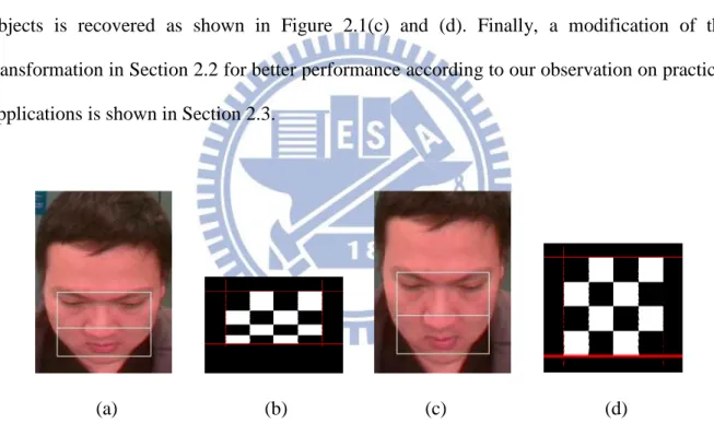
objects is recovered as shown in Figure 2.1(c) and (d). Finally, a modification of the

transformation in Section 2.2 for better performance according to our observation on practical

applications is shown in Section 2.3.

(a) (b) (c) (d)

Figure 2.1: Rectification results of Figures 1.2(c) and (d). (a)-(b) Obtained from transformation 1 discussed in Section 2.1. (c)-(d) Obtained from transformation 2 discussed in Section 2.2.

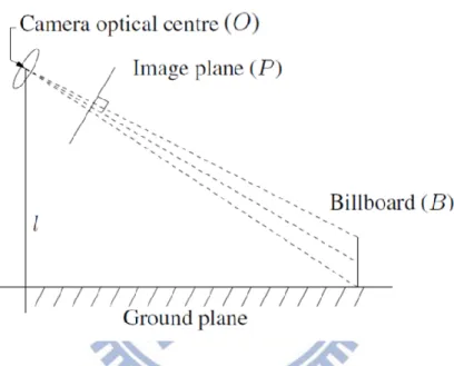
For better understanding of the basic idea of the proposed method, we first describe how

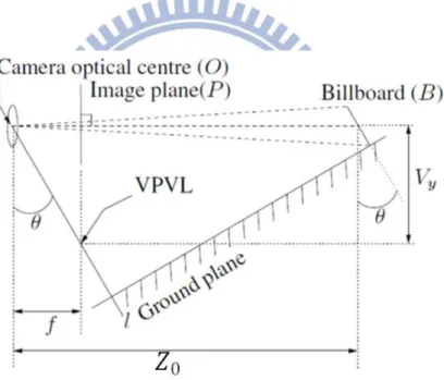
an object is captured by a surveillance camera. As shown in Figure 2.2, assume the camera is

located relatively higher than the object and its optical axis is not horizontal. Suppose there is

a square billboard standing vertically in front of the camera, with the pattern on the billboard

(17)

8

in Figure 1.2(d). Furthermore, the extension of vertical lines on the billboard will meet at a

single point in the image plane.

For simplicity, in the following discussion we assume that the image center is the origin

of the image plane, and the VPVL, V = ( ), can be derived from images of vertical lines via simple camera calibration. Additionally, each image is assumed to be rotated in advance

such that .

Figure 2.2: The relation between the camera, a standing billboard, and the ground plane, with the camera represented by its lens for simplicity. The billboard is assumed to be facing the vertical line containing the camera center.

(18)

9

2.1 Transformation 1

For the surveillance system described in Figure 2.2, we find that all square patterns on

the billboard, B, are transformed to trapezoids in the image plane, P, as shown in Figure

1.2(d). An intuitive way of image rectification is to make all lines pointing to VPVL vertically

parallel. To this end, we propose our first transformation and explain it as follows. Consider

Figure 2.3, where we would like to make an image, Figure 2.3(b) from the original image,

Figure 2.3(a). In particular, we would like to transform two horizontal line segments, and , in Figure 2.3(a) into and in Figure 2.3(b), respectively such that and are still horizontal and have the same length where O and o are the image center of

Figure 2.3(a) and (b). According to triangle geometry and simple calculation, we have

(2.1) (2.2)

In general we can define a transformation such that for each pixel (x, y) in Figure 2.3(b),

its content can be obtained at position (X, Y) in Figure 2.3(a) such that

(2.3)

In Figure 2.1(b) we can see that each trapezoid can be recovered as a rectangle, but not a

square. Moreover, a white block near the top is much larger than that near the bottom,

resulting in rectangles of different heights. At last Figure 2.4 shows an example of image

(19)

10

(a) (b)

Figure 2.3: An illustration diagram for transform 1. (a) Image before rectified. (b) Image after rectified.

(a) (b)

(20)

11

2.2 Transformation 2

In order to further recover the aspect ratio of an object, a novel image transformation is

presented in this section. To simplify the presentation, we first rotate the camera model shown

in Figure 2.2 to make the optical axis horizontal as illustrated in Figure 2.5, where θ is the tilt

angle, f is the focal length of the camera, l is a vertical line connect the optical center (O) and

the ground, and is distance from the optical center to the pixel which is the intersection of

the optical axis and the billboard (B). Furthermore, we set the origin of the 3D coordinate

system to be the optical center, with the z-axis to the right, the y-axis pointing downward, and

x-axis pointing out of the paper.

Figure 2.5: A rotation of Figure 2.2, to make the optical axis of the camera horizontal.

As shown in Figure 2.6, the value of the unknown parameter f can be found as

√ (2.4)

where F is the focal length in standard metric units, L is the size of the image sensor, and

(21)

12

Figure 2.6: An illustration showing the relationship between the image sensor and the image.

To investigate the relation between the billboard (B) and the image plane (P), let

(2.5)

where represents the 3D coordinates and represents 2D coordinates of a pixel on B.

Moreover, let denote the 3D coordinates of a pixel on the image plane (P), we have

(2.6)

Because P is parallel to the XY-plane of the 3D coordinate, is also the 2D coordinates of this corresponding pixel on P. Thus we can define an image transformation

(22)

13

where with being the coordinates of the transformed pixel. Finally, an example of image rectification of transformation 2 is shown in Figure 2.7.

In this transformation, affects only the scale of transferred image and can be

assigned with an arbitrary value per user’s requirement. On the other hand, for the remaining

unknown θ in equation (2.7), we can derive and as:

√ √ (a) (b)

(23)

14

2.3 Transformation 3

One characteristic of transformation 2 is that it is only valid for billboards parallel to the

XY-plane in the 3D coordinate. However, in most applications we are interested in all people facing to l in Figure 2.2. For example, if a camera is installed above an entrance, we are more

interested in people walking toward the entrance. Besides, people facing l also provide more

frontal face information and are thus more valuable. To make the proposed method more

suitable for any billboard facing l, we further propose a modified version, namely

transformation 3, of transformation 2 such that after the transformation, all pixels on image

plane (P) with the same distance to VPVL will be mapped to the same horizontal line in the

recovered image. The difference between results of transformation 2 and 3 is also illustrated

in Figure 2.8. In Figure 2.8 an image containing a person facing to l but not to the XY-plane is

rectified by transformation 2 and 3 respectively. For better illustrations, we draw a green line

on the person's eyes. It is obvious that the green line in the result of transformation 2 (Figure

2.8(a)) is not horizontal while in Figure 2.8(b) the green line is nearly horizontal and thus the

face in Figure 2.8(b) is more close to a normal face.

(a) (b)

Figure 2.8: Rectified image of Figure 1.1(b) by transformation 2 and 3. (a) Result of transformation 2. (b) Result of transformation 3.

(24)

15

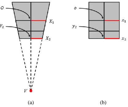
Figure 2.9 explains how the corresponding pixels in the original image can be found

according to the above description of transformation 3. In Figure 2.9 several corresponding

lines and pixels in transformation 3 (Figure 2.9(b)) and in the original image (Figure 2.9(a))

are illustrated. Specifically, the and represent the lines with in the original image and transformation 3, respectively. Now we show that for the pixel in Figure 2.9(b),

how to find its corresponding pixel in Figure 2.9(a). Given the pixel , we first find the pixel which is located at the central vertical line and has the same y-coordinate as . According to transformation 2 we know that comes from the pixel in the original

image. Then we rotate around the VP by which is proportional to the distance, , between and as : [ ] [ ] [ ] [ ] (2.9) (a) (b)

Figure 2.9: Relation between original image and rectified image by transformation 3. (a) Original image. (b) Rectified image by transformation 3.

(25)

16

Notice that and are both 0 and hence can be ignored. After combining Equation (2.9) as well as equation (2.7) of the transformation 2, we derive the formulation of

transformation 3:

( ) (

)

( ) (

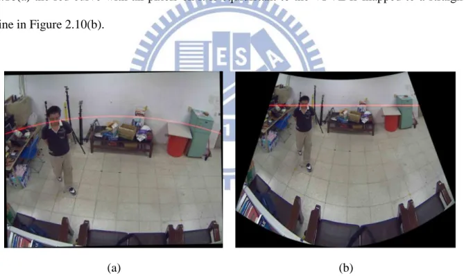
) where represents a pixel on rectified image and represents a pixels on plane P. An example of the transformation result is shown in Figure 2.10, where in Figure

2.10(a) the red curve with all pixels on it is equidistant to the VPVL is mapped to a straight

line in Figure 2.10(b).

(a) (b)

(26)

17

Chapter 3 Method for Reducing False Alarms

In this chapter we try to reduce false alarms for better detection performance. We

propose to use skin detection for its efficiency. The skin detection is carried only on regions

of candidates found by face detectors to further reduce the computation demand. In Section

3.1, the skin detection adopted in our system in introduced. The complete process and the

final results are present in Section 3.2.

3.1 Review of Skin Detection

In the work proposed by Garcia et al. [16], a skin color sub-space in YCbCr space is

figured out for detection of skin regions in MEPG streams and JPEG images. A data set

containing 950 skin colors samples is used in order to approximate the color sub-space.

These samples are extracted from various still images and video frames, covering a large

range of skin color appearance caused by different races and different lighting conditions.

Different from prior work, Garcia et al. propose to use varying intensity (Y) values to deal

with strong lighting variations as they notice that the skin color distribution turns out to be

(27)

18

distribution borders in the extreme light and dark cases, the authors actually propose two

groups of planes equations depending on two areas of the color space, separated by the

horizontal plane Y = 128. Their proposed planes equations are present in equation (3.1) while

two skin color sub-spaces defined by equation (3.1) according to two different Y values are

shown in Figure 3.1.

(a)

(b)

(c)

Figure 3.1: Skin color region define by [16] at Y = 110 and Y = 140. (a) YCbCr plane at different Y value. (b) Skin region define by equation 3.1. (c) Skin colors at different Y value.

(28)

19

3.2 Skin Color Percentage in Candidate Regions

(a)

(b) (c) (d) (e) (f)

Figure 3.2: (a) A picture with five candidate regions. (b) 0% skin color percentage in region 1. (c) 33% skin color percentage in region 2. (d) 0% skin color percentage in region 3. (e) 79% skin color percentage in region 4. (f) 0% skin color percentage in region 5.

In this section, we demonstrate how to reduce false alarms with skin detection and get a

better detection performance. For each image frame, we first find several candidates by the

face detector. Then we exploit the skin detection method mentioned in section 3.1 to find skin

pixels among regions of these candidates. Finally a candidate is taken out if the percentage of

skin pixels in the region under it is less than a threshold. Take Figure 3.2 for example, in

Figure 3.2(a) five candidates are detected and marked with red squares. For each candidate

(29)

20

3.2(b)-(f). Therefore, we may take out some bad candidates if we can find a suitable threshold

for skin pixel percentage. In order to determine such a threshold that can separate true faces

and false alarms properly, two videos are tested, i.e., S10 for indoor environment and O5 for

outdoor environment, as shown in Figure 3.3. Table 3.1 and Table 3.2 show face detection

results for different threshold values for the two videos. One can see that when the threshold

is set between 10% and 40% for indoor environment (between 15% and 35% for outdoor

environment) best detection results can be achieved. With such thresholds, we keep almost as

many true positives as the origin while reduce most false positives.

And we set the threshold to 40% and show the comparison of face detection results on

another video with and without the false alarm detection in Figure 3.4. One can see that with

false alarm detection most false positives have been removed while the true faces are still

preserved.

(a)

(b)

(30)

21

Table 3.1: The detection results for S10 with different thresholds of skin pixel percentage.

TP FP FN origin 80 31 0 P>0% 80 9 0 P>5% 80 2 0 P>10% 80 0 0 P>15% 80 0 0 P>20% 80 0 0 P>25% 80 0 0 P>30% 80 0 0 P>35% 80 0 0 P>40% 80 0 0 P>45% 78 0 2 P>50% 63 0 17 P>55% 41 0 39 P>60% 19 0 61 P>65% 0 0 80 P>70% 0 0 80 P>75% 0 0 80 P>80% 0 0 80 P>85% 0 0 80 P>90% 0 0 80 P>95% 0 0 80 P=100% 0 0 80

(31)

22

Table 3.2: The detection results for O5 with different thresholds of skin pixel percentage.

TP FP FN origin 115 184 0 P>0% 115 80 0 P>5% 115 56 0 P>10% 115 6 0 P>15% 115 0 0 P>20% 115 0 0 P>25% 115 0 0 P>30% 115 0 0 P>35% 115 0 0 P>40% 112 0 3 P>45% 107 0 8 P>50% 102 0 13 P>55% 96 0 19 P>60% 85 0 30 P>65% 78 0 37 P>70% 70 0 45 P>75% 39 0 76 P>80% 14 0 101 P>85% 6 0 109 P>90% 0 0 115 P>95% 0 0 115 P=100% 0 0 115

(32)

23

(33)

24

Chapter 4 Experimental Results

In this chapter, we give four experiments to show how face detection can be improved

with the proposed method. We have tested our method on videos under three real

environments as well as on some synthesized images. In Section 4.1, the specifications of

cameras used in our experiments and the installation parameters are detailed. In Section 4.2,

we show some image samples from our testing videos. An experiment for comparison is

present in Section 4.3. In this experiment, the videos are simply rotated such that the new

position of the VPVL is at the horizontal center. The face detection results of our method with

or without reducing false alarms method on videos under real environments are reported in

Section 4.4 and in Section 4.5, respectively. Finally, in Section 4.6 we show the experiments

on synthesized images with multiple camera installation settings.

4.1 Environment Settings

Through our experiments two cameras, named as AXIS 207MW and VIVOTEK FD8161

according to their model names, are used. In the indoor experiments, the AXIS 207MW is

attached at the ceiling without any calibration and is located about 2.7 meters above the

ground plane, as shown in Figure 4.1. In the outdoor experiments, we install the VIVOTEK

FD8161 above an entrance also without any calibration. The height of the camera is about 2.5

(34)

25

(a) (b)

Figure 4.1: Camera AXIS 207MW settings. (a) Experimental environment. (b) Close-up view of camera.

(a) (b)

(35)

26

4.2 Video Demonstration

We have captured 25 videos and use them in our experiments. As mentioned previously,

our experiments contain videos both on an indoor environment and on an outdoor

environment. These videos have different resolutions according to the camera models and

thus have different resolutions on the two environments. In our experiments the resolutions of

the indoor and outdoor videos are 640x480 and 800x600, respectively. In all videos one or

multiple people walking and roughly toward the camera are captured. Furthermore, these

people start walking from different positions so that we can see faces with different sizes,

rotations, and distortions, in these videos.

(a) (b) (c) (d)

(e) (f) (g) (h)

(i) (j)

Figure 4.3: Frame examples of a single person walking in the laboratory. (a) Video S1. (b) Video S2. (c) Video S3. (d) Video S4. (e) Video S5. (f) Video S6. (g) Video S7. (h) Video S8. (i) Video S9. (j) Video S10.

(36)

27

(a) (b) (c) (d)

(e) (f) (g)

Figure 4.4: Frame examples of multi people walking in the laboratory. (a) Video M1. (b) Video M2. (c) Video M3. (d) Video M4. (e) Video M5. (f) Video M6. (g) Video M7.

(a) (b) (c) (d)

(e) (f) (g) (h)

Figure 4.5: Frame examples of a single person walking in the outdoor environment. (a) Video O1. (b) Video O2. (c) Video O3. (d) Video O4. (e) Video O5. (f) Video O6. (g) Video O7. (h) Video O8.

(37)

28

4.3 Experiment 1 – Face Detection using Image Rotation

In this section, we present a simple method using only image rotation to improve face

detection with a surveillance camera. Based on the observation that faces in directions other

than the front of the camera seem like faces with in-plane rotations, to treat them just like

in-plane rotated faces like [14, 15] is an intuitive way. In [14, 15], faces with rotations in

different degrees are detected by rotated detectors. Unlike them, for easier implementation,

we instead rotate the image and repeat the detection procedure several times.

To decide the amount of the angular shift in each face detection procedure, we first

investigate the limitation of the frontal face detector, which is proposed in [17] and provided

in OpenCV, on in-plane rotations. A subset of the MUCT face database [18] is used in this

testing. More specifically, we use images captured by the camera "e" as shown in Figure 4.6.

There are total 751 images in the database and each subject is captured under 2 to 3 different

lightings as shown in Figure 4.7. In our testing each image is rotated 360 times with the step

of one degree and then the face detection results are carried out on all rotated versions. The

detection result of an image with all its rotated versions is shown in Figure 4.8 where the

maximum continuous region in which the face detection succeeds is of 48 degree. With the

same procedure on all images, we have the result that the smallest maximum continuous

region is of 28 degree and the average maximum continuous region is of 47.47 degree.

(38)

29

(a) (b) (c)

Figure 4.7: Three different lighting for a person in MUCT face database captured by camera e.

Figure 4.8: The testing result of Figure 4.7(a). 1=face was detected; 0=no face was detected. 22-(-25)+1=48, 48 is the maximum rotation in plane degree result for Figure 4.7(a).

Although the face detector is proved effective for faces rotated up to ±23.7 degree (half

of the average result 47.47), we take a relatively conservative rotation step of 15 degree in our

experiments. The maximum in-plane rotation of faces in our videos is about +24.8 degree,

thus it should be enough to rotate the images by ±15 degrees to deal with all in-plane rotations

occurred here. However, we also rotate images by ±30 degree and merge the results for more

robustness. An example of face detection on an image in rotations of different degrees is

shown in Figure 4.9. In Figure 4.9 the face detector can detect only one face in the original

image. In the meantime, the remaining two faces are detected in the -15 and -30 degree

rotated versions separately. It is obvious that more faces can be found if we provide more

(39)

30

(a) (b) (c)

(d) (e)

Figure 4.9: Example of rotating image. (a) Origin image. (b) Rotate -15 degree. (c) Rotate 15 degree. (d) Rotate -30 degree. (e) Rotate 30 degree.

By combining results in different rotations, we have the result shown in Figure 4.10. One

can see that although more faces are detected, the number of false positives is also increased.

(a) (b)

Figure 4.10: Combine the detection results of Figure 4.9 into one image. (a) Combine Figure 4.9(a)-(c) and 2 TP/FP in the image. (b) Combine Figure 4.9(a)-(e) and 3 TP/FP in the image.

(40)

31

Finally we show the detection results in Table 4.1 ~ Table 4.3. Where O represents the

origin method without any preprocessing on images; R1 represents combining the results on

the origin images and on the 15-degree rotated version; and R2 represents combining results

on the origin images, 15-degree rotated version and 30-degree rotated version. In the table, we

give precision and recall to show the detection performance. One can see that the more rotated

images are added, the higher recall and lower precision will be. In Table 4.4 we give the

average results across all videos. It is obviously to see that R2 has the best recall but the

lowest precision in most groups.

Table 4.1: Face detection results of S1 ~ S10 videos by image rotation.

S1 S2 S3 S4

Recall Precision Recall Precision Recall Precision Recall Precision

O 100% (126/126) 61.1% (126/206 30.5% (37/121) 40.6% (37/91) 38.8% (33/85) 27.5% (33/120) 8.8% (8/90) 7.7% (8/95) R1 100% (126/126) 49.6% (126/254) 99.1% (120/121) 55.8% (120/125) 96.4% (82/85) 34.4% (82/238) 97.7% (88/90) 35.3% (88/249) R2 100% (126/126) 47.0% (126/268) 99.1% (120/121) 50.0% (120/120) 96.4% (82/85) 32.2% (82/254) 100% (90/90) 33.4% (90/269) S5 S6 S7 S8

O 1.8% (1/55) 2.4% (1/41) 22.8% (13/57) 22.0% (13/59) 1.1% (1/85) 1.4% (1/71) 100% (79/79) 63.7% (79/124) R1 98.1% (54/55) 38.8% (54/139) 98.2% (56/57) 33.5% (56/167) 97.6% (83/85) 36.2% (83/229) 100% (79/79) 51.9% (79/152) R2 98.1% (54/55) 35.0% (54/154) 100% (57/57) 32.3% (57/176) 97.6% (83/85) 34.2% (83/242) 100% (79/79) 45.6% (79/173) S9 S10

Recall Precision Recall Precision

O 95.5% (86/90) 61.4% (86/140) 100% (80/80) 72.0% (80/111) R1 100% (90/90) 39.1% (90/230) 100% (80/80) 42.1% (80/190) R2 100% (90/90) 35.1% (90/256) 100% (80/80) 34.0% (80/245)

(41)

32

Table 4.2: Face detection results of M1 ~ M7 videos by image rotation.

M1 M2 M3 M4

O 42.2% (76/180) 69.0% (76/110) 50.4% (58/115) 71.6 % (58/81) 50.0% (62/124) 65.2% (62/95) 51.9% (109/210) 74.6% (109/146) R1 66.6% (120/180) 60.3% (120/199) 62.6% (72/115) 56.6% (72/127) 76.6% (95/124) 59.3% (95/160) 77.6% (163/210) 73.7% (163/221) R2 75.0% (135/180) 48.9% (134/276) 79.1% (91/115) 45.5% (91/200) 89.5% (111/124) 44.4% (111/250) 83.3% (175/210) 55.2% (175/317) M5 M6 M7

Recall Precision Recall Precision Recall Precision

O 46.9% (123/262) 75.9% (123/162) 62.2% (79/127) 60.7% (79/130) 61.4% (129/210) 61.1% (129/211) R1 69.4% (182/262) 67.1% (182/271) 69.2% (88/127) 48.3% (88/182) 69.5% (146/210) 51.2% (146/285) R2 77.1% (202/262) 51.5% (202/392) 77.9% (99/127) 44.7% (99/221) 75.2% (158/210) 48.0% (158/329)

Table 4.3: Face detection results of O1 ~ O8 videos by image rotation.

O1 O2 O3 O4

O 1.1% (1/86) 1.1% (1/91) 91.1% (82/90) 53.5% (82/153) 100% (90/90) 56.2% (90/160) 91.2% (73/80) 49.3% (73/148) R1 65.1% (56/86) 22.7% (56/246) 91.1% (82/90) 31.1% (82/263) 100% (90/90) 37.8% (90/238) 93.7% (75/80) 41.2% (75/182) R2 70.9% (61/86) 19.9% (61/306) 91.1% (82/90) 29.0% (82/282) 100% (90/90) 33.5% (90/268) 93.7% (75/80) 36.7% (75/204) O5 O6 O7 O8

O 93.0% (107/115) 58.4% (107/183) 98.9 % (94/95) 48.9% (94/192) 98.2% (113/115) 70.1% (113/161) 86.8% (139/160) 57.2% (139/243) R1 97.3% (112/115) 36.3% (112/308) 98.9% (94/95) 27.5% (94/341) 100% (115/115) 62.8% (115/183) 91.2% (146/160) 45.7% (146/319) R2 97.3% (112/115) 30.2% (112/370) 98.9% (94/95) 24.2% (94/388) 100% (115/115) 57.7% (115/199) 91.2% (146/160) 36.5% (146/400)

(42)

33

Table 4.4: Average detection results of image rotation method.

S1 ~ S10 videos M1 ~ M7 videos O1 ~ O8 videos All 25 videos

O 49.9% 35.9% 52.1% 68.3% 82.5% 49.3% 61.5% 51.2%

R1 98.7% 41.6% 70.2% 59.5% 92.1% 38.1% 87.0% 46.4%

R2 99.1% 37.8% 79.5% 48.3% 92.8% 33.4% 90.4% 39.8%

4.4 Experiment 2 – Face Detection based on Image Rectification

In this section, we show the detection performance by the proposed image rectification

methods. The results are reported in Table 4.5 ~ Table 4.8. Where O means the origin method

without any preprocessing on images; T1 means transformation 1; T2 means transformation 2;

and T3 means transformation 3. Again, we give precision and recall to show the detection

performance. Some images with different rectifications and face detection result are present in

Figure 4.11~4.13.

(a) (b) (c) (d)

(43)

34

In Table 4.8 we find that the face detection performances are generally improved by the

proposed methods. With the proposed three transformations the overall recall are improved

from 0.615 to 0.781, 0.837, and 0.905 separately. As the results show, transformation 3 has

the best recall. We also find that transformation 3 is very stable through all directions.

Table 4.5: Face detection results of S1 ~ S10 videos by image rectification.

S1 S2 S3 S4

O 100% (126/126) 61.1% (126/206) 30.5% (37/121) 40.6% (37/91) 38.8% (33/85) 27.5% (33/120) 8.8% (8/90) 7.7% (8/95) T1 100% (126/126) 78.2% (126/161) 81.8% (99/121) 66.4% (99/149) 83.5% (71/85) 59.1% (71/120) 77.7% (70/90) 56.0% (70/125) T2 100% (126/126) 62.3% (126/202) 98.3% (119/121) 59.8% (119/199) 90.5% (77/85) 30.9% (77/249) 94.4% (86/90) 34.2% (86/90) T3 100% (126/126) 43.9% (126/287) 96.6% (117/121) 42.7% (117/274) 97.6% (83/85) 52.2% (83/159) 98.8% (89/90) 47.5% (89/187) S5 S6 S7 S8

O 1.8% (1/55) 2.4% (1/41) 22.8% (13/57) 22.0% (13/59) 1.1% (1/85) 1.4% (1/71) 100% (79/79) 63.7% (79/124) T1 98.1% (54/55) 65.0% (54/83) 98.2% (56/57) 63.6% (56/98) 81.1% (69/85) 56.1% (69/123) 100% (79/79) 57.2% (79/138) T2 94.5% (52/55) 33.7% (52/154) 98.2% (56/57) 33.9% (56/165) 91.7% (78/85) 32.2% (78/242) 100% (79/79) 34.2% (79/231) T3 100% (55/55) 49.1% (55/112) 100% (57/57) 50.4% (57/113) 98.8% (84/85) 48.5% (84/173) 100% (79/79) 46.7% (79/169) S9 S10

O 95.5% (86/90) 61.4% (86/140) 100% (80/80) 72.0% (80/111) T1 78.8% (71/90) 65.7% (71/108) 100% (80/80) 62.9% (80/127) T2 92.2% (83/90) 33.2% (83/250) 100% (80/80) 36.7% (80/218) T3 100% (90/90) 49.1% (90/183) 100% (80/80) 54.7% (80/146)

(44)

35

Table 4.6: Face detection results of M1 ~ M7 videos by image rectification.

M1 M2 M3 M4

O 42.2% (76/180) 69.0% (76/110) 50.4% (58/115) 71.6% (58/81) 50.0% (62/124) 65.2% (62/95) 51.9% (109/210) 74.6% (109/146) T1 55.5% (100/180) 67.1% (100/149) 60.0% (69/115) 51.8% (69/133) 65.3% (81/124) 60.0% (81/135) 70.9% (149/210) 60.8% (149/245) T2 61.1% (110/180) 55.2% (110/199) 69.5% (80/115) 44.6% (80/179) 66.9% (83/124) 44.6% (83/186) 80.0% (168/210) 54.9% (165/306) T3 74.4% (134/180) 62.3% (134/215) 74.7% (86/115) 51.8% (86/166) 89.5% (111/124) 57.2% (111/196) 84.2% (177/210) 51.6% (177/343) M5 M6 M7

O 46.9% (123/262) 75.9% (123/162) 62.2% (79/127) 60.7% (79/130) 61.4% (129/210) 61.1% (129/211) T1 59.1% (155/262) 58.4% (155/265) 66.1% (84/127) 70.0% (84/120) 54.7% (115/210) 61.5% (115/187) T2 64.1% (168/262) 47.0% (168/357) 74.0% (94/127) 64.3% (94/146) 59.0% (124/210) 48.2% (124/256) T3 77.4% (203/262) 49.5% (203/410) 79.5% (101/127) 59.7% (101/169) 74.2% (156/210) 48.3% (156/323) (a) (b) (c) (d)

(45)

36

Table 4.7: Face detection results of O1 ~ O8 videos by image rectification.

O1 O2 O3 O4

O 1.1% (1/86) 1.1% (1/91) 91.1% (82/90) 53.5% (82/153) 100% (90/90) 56.2% (90/160) 91.2% (73/80) 49.3% (73/148) T1 32.5% (28/86) 16.7% (28/167) 85.5% (77/90) 48.4% (77/159) 100% (90/90) 52.9% (90/170) 86.2% (69/80) 53.9% (69/128) T2 50.0% (43/86) 19.2% (43/224) 91.1% (82/90) 37.1% (82/221) 97.7% (88/90) 41.7% (88/211) 92.5% (74/80) 46.8% (74/158) T3 69.7% (60/86) 26.3% (60/228) 91.1% (82/90) 34.0% (82/241) 100% (90/90) 38.4% (90/234) 98.7% (79/80) 40.9% (79/193) O5 O6 O7 O8

O 93.0% (107/115) 58.4% (107/183) 98.9% (94/95) 48.9% (94/192) 98.2% (113/115) 70.1% (113/161) 86.8% (139/160) 57.2% (139/243) T1 93.0% (107/115) 58.7% (107/182) 83.1% (79/95) 40.1% (79/197) 95.6% (110/115) 71.9% (110/153) 88.1% (141/160) 53.0% (141/266) T2 94.7% (109/115) 49.3% (109/221) 87.3% (83/95) 29.9% (83/277) 98.2% (113/115) 58.8% (113/192) 88.7% (142/160) 42.0% (142/338) T3 95.6% (110/115) 37.4% (110/294) 98.9% (94/95) 28.9% (94/325) 100% (115/155) 66.8% (115/172) 93.7% (150/160) 53.9% (150/278) (a) (b) (c) (d)

(46)

37

Table 4.8: Average detection results of image rectification method.

O 49.9% 35.9% 52.1% 68.3% 82.5% 49.3% 61.5% 51.2%

T1 89.9% 63.0% 61.6% 61.3% 83.0% 49.4% 78.1% 57.9%

T2 95.9% 39.1% 67.8% 51.2% 87.5% 40.6% 83.7% 43.6%

T3 99.1% 48.4% 79.1% 54.3% 93.4% 40.8% 90.5% 47.8%

Now we compare the proposed methods with the image rotation method mentioned in

the previous subsection. Comparing Table 4.4 and Table 4.8, we can see that T3 has better

recall and precision than R1 and R2. The computation times of different methods on three

different videos are shown in Table 4.9. Where T1 is 1.3 times slower than O; T2 and T3 are

almost 1.5 times slower than O. When compared with the image rotation method, we see that

T1, T2, and T3 on the contrary are over 1.8 and 3.3 times faster R1 and R2. This leads to the

conclusion that although image rotation can improve the detection performance, it also results

more false positives and computation times than our proposed methods.

Table 4.9: The computation time(s) of each face detection methods.

Frame Number O T1 T2 T3 R1 R2

S1 126 70.14 92.00 112.72 105.14 189.47 327.47

M1 90 47.44 69.57 77.19 71.48 132.91 217.20

(47)

38

4.5 Experiment 3 – Face Detection based on Image Rectification

with Reducing False Alarms Method

In this section, we show the face detection results by combining the false alarms

reducing method proposed in Chapter 3 with the transformation 3. As suggested in Section

3.2, we test two thresholds, 40 and 45, on percentage of skin region in this experiment. The

results are reported in Table 4.10 ~ 4.12. Where T3 denotes transformation 3; P0 means

reducing false alarms in T3 with the threshold 35%; P1 means reducing false alarms in T3

with the threshold 40%; and P2 means reducing false alarms in T3 with the threshold 45%. As

used in previous sections, we give precision and recall to show the detection performance.

Table 4.10: Face detection results of S1 ~ S10 videos by image rectification with reducing false alarms.

S1 S2 S3 S4

T3 100% (126/126) 43.9% (126/287) 96.6% (117/121) 42.7% (117/274) 97.6% (83/85) 52.2% (83159) 98.8% (89/90) 47.5% (89/187) P1 100% (126/126) 100% (126/126) 96.6% (117/121) 100% (117/117) 97.6% (83/85) 98.8% (83/84) 98.8% (89/90) 100% (89/89) P2 100% (126/126) 100% (126/126) 96.6% (117/121) 100% (117/117) 97.6 % (83/85) 100% (83/83) 98.8% (89/90) 100% (89/89) S5 S6 S7 S8

T3 100% (55/55) 49.1% (55/121) 100% (57/57) 50.4% (57/113) 98.8% (84/85) 48.5% (84/173) 100% (79/79) 46.7% (79/169) P1 100% (55/55) 98.2% (55/56) 100% (57/57) 100% (57/57) 98.8% (84/85) 100% (84/84) 100% (79/79) 100% (79/79) P2 100% (55/55) 100% (55/55) 100% (57/57) 100% (57/57) 98.8% (84/85) 100% (84/84) 100% (79/79) 100% (79/79) S9 S10

T3 100% (90/90) 49.1% (90/183) 100% (80/80) 54.7 % (80/146) P1 88.8% (80/90) 100% (80/80) 100% (80/80) 100% (80/80) P2 80.0% (72/90) 100% (72/72) 95.0% (76/80) 100% (76/76)

(48)

39

Table 4.11: Face detection results of M1 ~ M7 videos by image rectification with reducing false alarms.

M1 M2 M3 M4

T3 74.4% (134/180) 62.3% (134/215) 74.7% (86/115) 51.8% (86/166) 89.5% (111/124) 57.2% (111/196) 84.2% (177/210) 51.6% (177/343) P1 74.4% (134/180) 100% (134/134) 74.7% (86/115) 100% (86/86) 89.5% (111/124) 100% (111/111) 84.2% (177/210) 97.2% (177/185) P2 74.4% (134/180) 100% (134/134) 74.7% (86/115) 100% (86/86) 89.5% (111/124) 100% (111/111) 84.2% (177/210) 100% (177/177) M5 M6 M7

T3 77.4% (203/262) 49.5% (203/410) 79.5% (101/127) 59.7% (101/169) 74.2% (156/210) 48.3% (156/323) P1 77.4% (203/262) 97.6% (203/208) 79.5% (101/127) 99.0% (101/102) 73.8% (155/210) 98.7% (155/157) P2 77.4% (203/262) 100% (203/203) 79.5% (101/127) 100% (101/101) 73.8% (155/210) 99.3% (155/156)

Table 4.12: Face detection results of O1 ~ O8 videos by image rectification with reducing false alarms.

O1 O2 O3 O4

T3 69.7% (60/86) 26.3% (60/228) 91.1% (82/90) 34.0% (82/241) 100% (90/90) 38.4% (90/234) 98.7% (79/80) 40.9% (79/193) P0 69.7% (60/86) 100% (60/60) 90.0% (81/90) 100% (81/81) 100% (90/90) 100% (90/90) 98.7% (79/80) 100% (79/79) P1 69. % (60/86) 100% (60/60) 83.3% (75/90) 100% (75/75) 100% (90/90) 100% (90/90) 98.7% (79/80) 100% (79/79) O5 O6 O7 O8

T3 95.6% (110/115) 37.4% (110/294) 98.9% (94/95) 28.9% (94/325) 100% (115/115) 66.8% (115/172) 93.7% (150/160) 53.9% (150/278) P0 100% (115/115) 100% (115/115) 98.9% (94/95) 100% (94/94) 99.1% (114/115) 99.1% (114/115) 93.7% (150/160) 100% (150/150) P1 97.3% (112/115) 100% (112/112) 98.9% (94/95) 100% (94/94) 93.0% (107/115) 99.0% (107/108) 93.7% (150/160) 100% (150/150)

(49)

40

Table 4.13: Average detection results of image rectification with reducing false alarms.

T3 99.1% 48.4% 79.1% 54.3% 93.4% 40.8% 90.5% 47.8%

P0 - - - - 93.7% 99.8% 93.7% 99.8%

P1 98.0% 99.7% 79.0% 98.9% 91.8% 99.8% 89.6% 99.5%

P2 96.6% 100% 79.0% 99.9% - - 87.8% 99.9%

After the false alarm reducing process, one can see in Table 4.13 that the precision in all

videos has been improved to 0.9 and 1. In the meanwhile, the precision is enhanced by nearly

0.5 while the detection rate is only decreased less than 0.03. The computation times are

reported in Table 4.14, where P combining the false alarm reducing method with

transformation 3. As shown in Table 4.14, with the proposed false alarms reducing method

the computation time are only be increased by 1 second through the three videos, which is

about 0.01 second per frame.

Table 4.14: The computation time(s) of T3 and reducing false alarm method.

Video Frame Number T3 P

S1 126 105.14 106.94

M1 90 71.48 72.57

(50)

41

4.6 Experiment 4 – Face Detection in Synthetic Scene

In order to show how the proposed methods can work under different situations in an

efficient way, we build a synthetic scene by Autodesk MAYA for our experiments. With

MAYA we construct a scene containing 21 people and a camera. These virtual people are

positioned in three rows and spaced equally by one meter. Besides, we set the distance

between the camera and the person in the middle of the first row to 2.5 meters. An example of

these settings is shown in Figure 4.14 and some images captured by the camera are shown in

Figure 4.15.

(a) (b)

Figure 4.14: The environment of synthetic scene. (a) An aerial image of the synthetic scene. (b) A side view of the synthetic scene with camera at 3 meters height and 40 degree angle of depression.

(a) (b)

(51)

42 (a)

(b)

Figure 4.16: The detection rates of different transformations by different camera settings. (a) The detection rates from different transformations according to varying camera heights. (b) The detection rates from different transformations according to varying camera angles.

(52)

43 (a)

(b)

Figure 4.17: The detection rates of different face detection methods by different camera settings. (a) The detection rates from different face detection methods according to varying camera heights. (b) The detection rates from different face detection methods according to varying camera angles.

(53)

44

Because of the clean background with which no false alarm occurs in our experiment, we

only focus on the detection rate (recall) in the following. In this experiment we have five

heights, from 2m to 6m, and nine tilt angles, from , in the camera settings. The detection rates are plotted in Figure 4.16. In Figure 4.16(a), we show the detection rates with

different camera heights across all camera angles. In Figure 4.16 (b), conversely we show the

detection rates with different camera angles across all heights. Throughout the experiments

we see that best face detection result is obtained with transformation 3; the second is with

transformation 2; the third is with transformation 1; and with the original images we have the

worse result. We also add the detection result with the image rotation method introduced in

Section 4.3 for comparison which is shown in Figure 4.17. From it we can conclude that

transformation 3 is more suitable than all the rest methods in the common surveillance

(54)

45

Chapter 5 Conclusions and Future Works

In this chapter we give our conclusions of this thesis in Section 5.1 and some future

works in Section 5.2.

5.1 Conclusions

In this thesis we propose a novel method to improve face detection in a practical

condition with vanishing point-based image rectification. Our approach requires only the

position of the vanishing point of vertical lines or two vertical lines marked by the user.

Compare with the simple image rotation method, our method gives better results and requires

much less computational resource. For better detection performance, we further propose a

method for reducing false alarms by skin analysis. This method significantly decreases false

alarms and only causes negligible additional computation time. Through the proposed

framework, the face detection performance is significantly improved for common surveillance

camera installation.

5.2 Future Works

In our future works, a detection scheme which is more suitable for image rectified by the

proposed method is considered. For example, since the lower part of the rectified image is

generally enlarged, the minimal detection window could be set larger around there for better

efficiency. On the other hand, how to properly adopt a multi-view face model for face

detection is also considered. By these works, the integrity of the detection method can be

(55)

46

References

[1] Y. Ishii, H. Hongo, K. Yamamoto and Y. Niwa, "Face and head detection for a real-time

surveillance system," in Proc. International Conference on Pattern Recognition, vol.3,

pp.298-301, Aug. 2004.

[2] O. Arandjelovic and Roberto Cipolla, "An illumination invariant face recognition system

for access control using video," in Proc. British Machine Vision Conference, 2004.

[3] Lloyd A. B. Louw, "Automated face detection and recognition for a login system," M.S.

thesis, Dept. Science of Engineering, University of Stellenbosch, 2007.

[4] D.G. Lowe, "Object recognition from local scale-invariant features," in Proc. IEEE

International Conference on Computer Vision, vol.2, pp.1150-1157, 1999.

[5] M.F. Tappen, W.T. Freeman and E.H. Adelson, "Recovering intrinsic images from a

single image," IEEE Transactions on Pattern Analysis and Machine Intelligence, vol.27,

no.9, pp.1459-1472, Sept. 2005.

[6] I. Kemelmacher-Shlizerman and R. Basri, "3D Face Reconstruction from a Single Image

Using a Single Reference Face Shape," IEEE Transactions on Pattern Analysis and

Machine Intelligence, vol.33, no.2, pp.394-405, Feb. 2011.

[7] G. Fangi, G. Gagliardini and E.S. Malinverni, "Photointerpretation and small scale

stereoplotting with digitally rectified photographs with geometrical constraints,"

International Archives of the Photogrammetry, Remote Sensing and Spatial Information Sciences, pp. 160-167, 2001.

[8] F. Schaffalitzky and A. Zisserman, "Planar grouping for automatic detection of

vanishing lines and points," Image and Vision Computing, vol. 18, pp. 647-658, 2000.

[9] O. Chum and J. Matas, "Planar affine rectification from change of scale," in Proc. Asian

Conference on Computer Vision, Springer Berlin Heidelberg, pp. 347-360, 2011.

(56)

47

spectral analysis on the unit sphere," Pattern Recognition, vol. 35, no. 10, pp. 2141-2163,

2002.

[11] A.P. Witkin, "Recovering surface shape and orientation from texture," Artificial

intelligence, vol. 17, pp. 17-45, 1981.

[12] C. Rasmussen, "Texture-based vanishing point voting for road shape estimation," in

Proceedings of the British Machine Vision Conference, 2004.

[13] P. Viola and M. Jones, "Rapid object detection using a boosted cascade of simple

features," in Proc. IEEE International Conference on Computer Vision and Pattern

Recognition, vol.1, pp.511-518, 2001.

[14] B. Wu, H. Ai, C. Huang and S. Lao, "Fast rotation invariant multi-view face detection

based on real Adaboost," in Proc. IEEE International Conference on Automatic Face

and Gesture Recognition, pp.79-84, May 2004.

[15] C. Huang, H. Ai, Y. Li and S. Lao, "Vector boosting for rotation invariant multi-view

face detection," in Proc. IEEE International Conference on Computer Vision, vol.1,

pp.446-453, Oct. 2005.

[16] C. Garcia, G. Zikos and G. Tziritas, "Face detection in color images using wavelet

packet analysis," in Proc. International Conference on Multimedia Computing and

Systems, vol.1, pp.703-708, Jul. 1999.

[17] R. Lienhart, A. Kuranov and V. Pisarevsky, "Empirical analysis of detection cascades of

boosted classifiers for rapid object detection," Pattern Recognition, Springer Berlin

Heidelberg, pp.297-304, 2003.

[18] S. Milborrow, J. Morkel and F. Nicolls, "The muct landmarked face database," Pattern

應用基於消失點之影像校正於強健式人臉偵測

國

立

交

通

大

學

多媒體工程研究所

碩

士

論

文

應用基於消失點之影像校正於強健式人臉偵測

Vanishing Point-Based Image Rectification for Robust Face Detection

研 究 生：王靖賀

指導教授：莊仁輝 教授

應用基於消失點之影像校正於強健式人臉偵測

Vanishing Point-Based Image Rectification for Robust Face Detection

研 究 生：王靖賀 Student：Ching-Ho Wang

指導教授：莊仁輝 Advisor：Jen-Hui Chuang

國 立 交 通 大 學

多 媒 體 工 程 研 究 所

碩 士 論 文

應用基於消失點之影像校正

於強健式人臉偵測

學生：王靖賀 指導教授：莊仁輝 博士

國立交通大學

多媒體工程研究所碩士班

摘 要

Vanishing Point-Based Image Rectification for Robust Face Detection

Student：Ching-Ho Wang Advisor：Dr. Jen-Hui Chuang

Institute of Multimedia Engineering

National Chiao Tung University

Abstract

Acknowledgement

Contents

List of Figures

List of Tables

Chapter 1

Introduction

1.1 Motivation

1.2 Related Work

1.2.1 Image Rectification

1.2.2 Face Detection Techniques

1.3 Organization of thesis

Chapter 2

Vanishing Point-based Image Rectification

2.1 Transformation 1

2.2 Transformation 2

2.3 Transformation 3

Chapter 3

Method for Reducing False Alarms

3.1 Review of Skin Detection

3.2 Skin Color Percentage in Candidate Regions

Chapter 4

Experimental Results

4.1 Environment Settings

4.2 Video Demonstration

4.3 Experiment 1 – Face Detection using Image Rotation

4.4 Experiment 2 – Face Detection based on Image Rectification

4.5 Experiment 3 – Face Detection based on Image Rectification

with Reducing False Alarms Method

4.6 Experiment 4 – Face Detection in Synthetic Scene

Chapter 5

Conclusions and Future Works

5.1 Conclusions

5.2 Future Works

References

研究生：王靖賀

指導教授：莊仁輝教授

研究生：王靖賀 Student：Ching-Ho Wang

國立交通大學

多媒體工程研究所

碩士論文

學生：王靖賀指導教授：莊仁輝博士

摘要