數值模擬冷藏垂直開放櫃之氣簾對其動量及熱質傳特性影響研究

(1)

國立交通大學

機械工程學系

碩士論文

數值模擬冷藏垂直開放櫃之氣簾對其動量及熱質傳特

性影響研究

Effects of Air Curtains on Momentum, Heat and Mass Transfer in an

Open Vertical Refrigerated Display Cabinet- Numerical Simulation

研究生:

林君達

指導教授:

林清發博士

(2)

數值模擬冷藏垂直開放櫃之氣簾對其動量及熱質傳特

性影響研究

Effects of Air Curtains on Momentum, Heat and Mass Transfer in an

Open Vertical Refrigerated Display Cabinet- Numerical Simulation

研究生：林君達

Student ：Chun-Ta Lin

指導教授：林清發

Advisor ：Tsing-Fa Lin

國立交通大學

機械工程學系

碩士論文

A Thesis Proposal

Submitted to Institute of Mechanical Engineering

Collage of Engineering

National Chiao Tung University

In Partial Fulfillment of the Requirements

For the degree of

Master of Science

In

Mechanical Engineering

November 2005

Hsinchu, Taiwan, Republic of China

(3)

(4)

(5)

(6)

(7)

誌謝

時光飛逝，回首在新竹這幾年來的點點滴滴，與當年隻身到交大求學的我相比，在交大這充滿學術氣息的環境下似乎讓我在知識上成長茁壯許多。本論文之所以可以順利完成，首先要感謝的是指導老師林清發教授嚴謹及殷切的指導，使學生能培養出獨立思考、釐清並自行解決問題的能力；更在學生撰寫論文時，不辭辛勞逐字斧正文稿，在此獻上最高謝意。在研究所期間，要特別感謝工研院謝文德博士與趙令裕研究員及 PHOENICS 范乃文先生在 PHOENICS 軟體上的協助指導，亦要感謝博士班郭威伸、賴佑民、陳尚緯、謝汎鈞、張文瑞等博士班學長在生活及課業上指導與建議，使我受益匪淺，謝謝您們。建安、義祥、宇歆這群不只是求學中的同學，更是生活上的好朋友。研究所之所以能在緊湊忙碌又充滿歡樂中的氣氛中度過，即是靠這些同學兼好友的夥伴們相互協助幫忙，令我永生難忘。另外也要感謝奎銘、凱文、峻樟、政陞等一群努力的學弟妹幫忙及合作，希望你們能繼續保持實驗室優良傳統，並帶著實驗室進步。最後更要感謝父母及姊姊對於我無怨無悔付出及支持，使我可以無後顧之憂的專注於研究，並且可無憂無慮過求學生活。並特別要感謝女友佩諭的陪伴與體恤，生活最精采的部分是妳陪我渡過，不管在課業上或生活上的關心與支持使我有勇氣面對一切的困難挑戰。能與妳相處是我這輩子最大的幸福。最後，僅以本文獻給我所關心的人和所有關心我的人。今日我以交大為榮願他日交大以我為榮君達謹致 2006/6/30 于風城交大

(8)

數值模擬冷藏垂直開放櫃之氣簾之動量及熱質傳特性研究

研究生: 林君達指導老師: 林清發博士 國立交通大學 機械工程學系

中文摘要

本篇論文利用二維穩態數值模擬方法探討一之氣簾穿過一垂直開放展示櫃之溫度與溼度濃度特性影響研究；以商用套裝計算流體力學軟體 PHOENICS 對流體的統馭方程式進行求解，論文著重確認由相對溼度對流場的溫溼度濃度影響；針對不同氣簾出口寬度 5.0， 7.0， 10.0 及 12.0 cm，及氣簾長度 1.20 m 與展示櫃深度 0.57m，及出口流速 0.25 至 3.0 m/s，之冷卻氣簾包含兩種不同渦流結構之穩態開放櫃流場研究。其中氣簾出口與環境溫度分別為 5.0 及 25.0℃，溫度差為 20℃。氣簾出口及環境的相對溼度分別為 90%與 60%。結果指出在沒有加入溫度差及濃度差的效應下，展示櫃內為單一的 flow recirculation。當加入溫度及濃度的浮力效應時，氣簾將會改變方向，向展示櫃內 bending，且環境的濕暖空氣將滲入展示櫃內。當熱傳與質傳的浮慣比大到一個程度時，氣簾的 bending 將會碰到展示櫃內壁面，形成兩個不同方向旋轉的 flow recirculations。除此之外縮小氣簾出口寬度將會減緩氣簾的 bending。而進一步將氣簾出口環境方向偏移一個角度以及展示櫃內的垂直壁面 perforation 出風，也更有效的減緩氣簾的 bending 現象。在雙氣簾的設計中，氣簾的 bending 現象及環境的暖濕空氣可藉由內外氣簾分別使用較小及較大的出口寬度。除此之外內外氣簾的相對出口雷諾數再展示

(9)

櫃的效應有非單一的影響。並且在外氣簾偏移一個角度後也將有效的改善展示櫃的整體效能。

(10)

Effects of Air Curtains on Momentum, Heat and Mass Transfer in

an Open Vertical Refrigerated Display Cabinet- Numerical

Simulation

Student: Chun-Ta Lin Advisor: Prof. Tsing-Fa Lin Department of Mechanical Engineering

National Chiao Tung University

ABSTRACT

A steady two-dimensional numerical simulation is conducted in the present study to investigate the momentum, heat and mass transfer resulting from cold air curtain discharge over the open surface of a vertical open cavity, simulating that in a vertical refrigerated display cabinet. The commercial computational fluid dynamics software PHOENICS [25] is employed to solve the problem. Attention is focused on how the parameters associated with the air curtain affect the characteristics of the flow in the cabinet. Computations are performed for the jet speed at the air discharge grille varying from 0.25 to 3.0 m/s and injection slot width ranging from 0.05 to 0.12 m for the air discharge-to-return grille separation distance fixed at 1.20 m and for the cabinet depth of 0.57 m. The temperature difference between the air discharge and ambient is 20 ℃, corresponding to Tj = 5 ℃ and Tamb = 25 ℃. The relative humidities at the air discharge and ambient are respectively fixed at 90% and 60%. Effects of various parameters on the flow, thermal and solutal characteristics in the cabinet are examined in detail. The results indicate that for the limiting case in the absence of the buoyancy force the cabinet is dominated by a single large flow recirculation. But when the Richardson numbers (buoyancy-to

(11)

-inertia ratios) exceed certain levels, the bending of the air curtain toward the cabinet core and the intrusion of the warm moist air from the ambient into the cabinet become significant. At high Rit and Rim the air curtain bending can be large enough

to induce two counter-rotating flow recirculations in the cabinet. Besides, a reduction in the injection slot width is found to result in a milder air curtain bending and warm air intrusion. Similar effects can be obtained by inclining the air curtain at the discharge grille slightly toward the ambient and by injecting the air flow into the cabinet from the back panel perforations.

In a two air-curtain design, the air curtain bending and warm air intrusion can be reduced by a larger inner jet width and a smaller outer jet width at the discharge grille for a fixed total width of the two jets. Besides, the relative magnitudes of the inner and outer jet Reynolds numbers are noted to produce nonmonotonic influence on the performance of the cabinet. Moreover, it is found that inclining the outer air jet toward the ambient with the inner jet still in the vertically downward direction can improve the cabinet performance.

(12)

LIST OF FIGURES

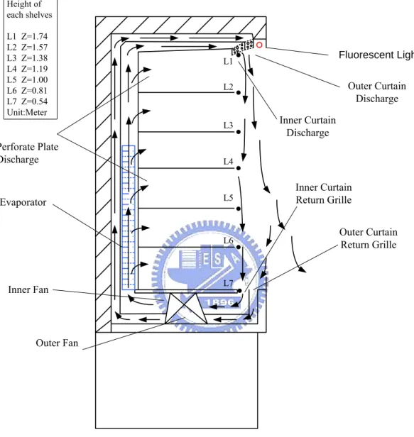
Fig. 1.1 Schematic diagram of a multi-deck open refrigerated display case ---8

Fig. 2.1 Physical model for a vertical refrigerated display case.--- 21

Fig. 2.2 Schematic diagram illustrating the geometry and some boundary conditions.--- 22

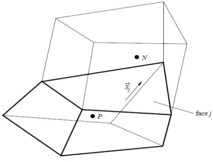
Fig. 3.1 The locations of the centred node P in a typical cell and centred node N in the neighbor cell. --- 29

Fig. 3.2 The upwind differencing with node labeling for flux discretization.--- 30

Fig. 3.3 Flow chart for the simulation procedures. --- 31

Fig. 3.4 The mesh distribution for the entire computational domain. --- 32

Fig. 3.5 The horizontal variations of the steady velocity magnitude at the selected locations on the line z = 1.7 m predicted from three different grids for bj = 0.1 m, Vj = 1.5 m/s, ΔT = 20 ℃ and N = 0.--- 33

Fig. 3.6 Velocity vector maps at steady state for bj = 0.1 m, Reb = 9,548, Grt = 4.61 × 109, and Grm = 2.94 × 108 predicted from the grids with (a) 8,550 cells, (b) 21,315 cells and (c) 16,764 cells. --- 34

Fig. 3.7 Isotherms at steady state for bj = 0.1 m, Reb = 9,548, Grt = 4.61 × 109, and Grm = 2.94 × 108 predicted from the grids with (a) 8,550 cells, (b) 21,315 cells and (c) 16,764 cells. --- 35

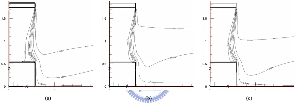
Fig. 3.8 Iso-concentration lines at steady state for bj = 0.1 m, Reb = 9,548, Grt = 4.61 × 109, and Grm = 2.94 × 108 predicted from the grids with (a) 8,550 cells, (b) 21,315 cells and (c) 16,764 cells. --- 36

Fig. 3.9 Conduction heat flux at x = 0.52 m at steady state for bj = 0.1 m, Reb = 9,548, Grt = 4.61 × 109, and Grm = 2.94 × 108 predicted from the grids with (a) 8,550 cells, (b) 21,315 cells and (c) 16,764 cells.--- 37 Fig. 3.10 Convection heat flux at x = 0.52 m at steady state for bj = 0.1 m, Reb =

(15)

9,548, Grt = 4.61 × 109, and Grm = 2.94 × 108 predicted from the grids with (a) 8,550 cells, (b) 21,315 cells and (c) 16,764 cells.--- 38 Fig. 3.11 Velocity vector maps at steady state for bj = 0.1 m, Reb = 9,548, Grt = 4.61

× 109, and Grm = 2.94 × 108 predicted with the domain size of (a) 3 × 2.5 m2, (b) 6 × 4.5 m2 and (c) 4.61 × 3.3 m2. --- 39 Fig. 3.12 Isotherms at steady state for bj = 0.1 m, Reb = 9,548, Grt = 4.61 × 109, and

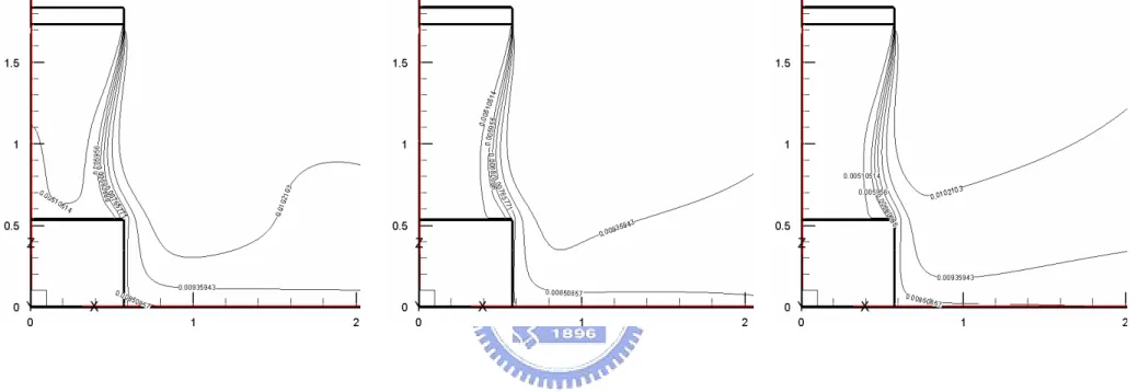
Grm = 2.94 × 108 predicted with the domain size of (a) 3 × 2.5 m2, (b) 6 × 4.5 m2 and (c) 4.61 × 3.3 m2. --- 40 Fig. 3.13 Iso-concentration lines at steady state for bj = 0.1 m, Reb = 9,548, Grt =

4.61 × 109, and Grm = 2.94 × 108 predicted with the domain size of (a) 3 × 2.5 m2, (b) 6 × 4.5 m2 and (c) 4.61 × 3.3 m2. --- 41 Fig. 3.14 Vector velocity maps in the steady cavity flow for the case with bj = 0.1 m,

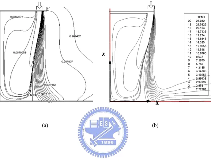
H = 2.0 m, Reb = 18,371, Grt = 2.7 × 1010, Pr = 0.71 and N = 0 predicted from (a) Chen & Yuan (2005) and (b) present study.--- 42 Fig. 3.15 Isotherms in the steady cavity flow for the case with bj = 0.1 m, H = 2.0 m,

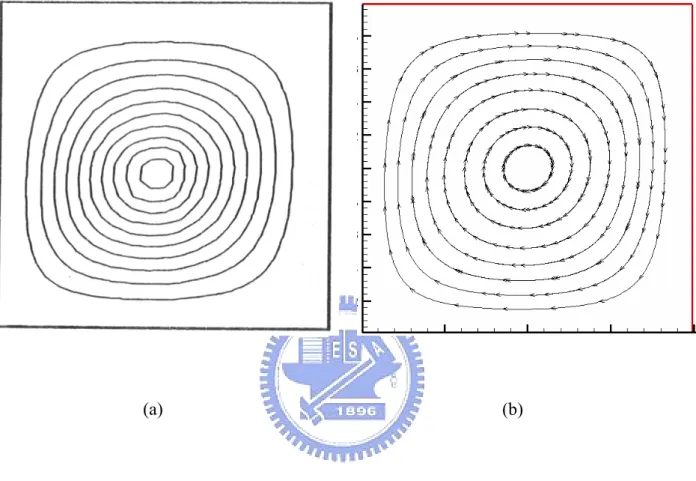
Reb = 18,371, Grt = 2.7 × 1010, Pr = 0.71 and N = 0 predicted from (a) Chen & Yuan (2005) and (b) present study. --- 43 Fig. 3.16 Streamlines in the steady square cavity flow for the case with H = L = 0.02

m, Grt = 103 , Grm = 1.43 × 103, Pr = 0.71 predicted from (a) Lai (1989) and (b) present study. --- 44 Fig. 3.17 Isotherms in the steady square cavity flow for the case with H = L = 0.02 m,

Grt = 103 , Grm = 1.43 × 103, Pr = 0.71 predicted from (a) Lai (1989) and (b) present study. --- 45 Fig. 3.18 Iso-concentration lines in the steady square cavity flow for the case with H

= L = 0.02 m, Grt = 103 , Grm = 1.43 × 103, Pr = 0.71 predicted from (a) Lai (1989) and (b) present study. --- 46

(16)

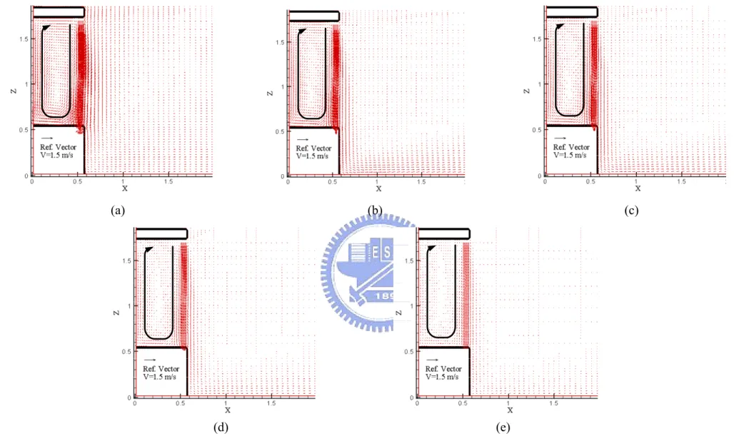
Fig. 4.1 Velocity vector maps for steady cavity flow for bj = 0.1 m, Grt = 0 (ΔT = 0 ℃) and N = 0 for Reb = (a)9,548 (Vj = 1.5 m/s), (b) 6,365 ( Vj = 1.0 m/s), (c) 5,092 ( Vj = 0.8 m/s), (d) 3,183 ( Vj = 0.5 m/s) and (e) 1,910 ( Vj = 0.3 m/s). --- 59 Fig. 4.2 Velocity vector maps for steady cavity flow for bj = 0.07 m, Grt = 0 (ΔT =

0℃), and N = 0 for Reb = (a)9,548 (Vj = 2.143 m/s), (b) 6,365 ( Vj = 1.428 m/s), (c) 5,092 ( Vj = 1.143 m/s), (d) 3,183 ( Vj = 0.714 m/s) and (e) 1,910 ( Vj = 0.428 m/s).--- 60 Fig.4.3 Steady recirculating flow pattern from Chen & Yuan [10] for H / bj = 20, Grt

= 2.7 × 1010 and N = 0 for (a) Rit = 0.2 and (b) Rit =0.32.--- 61 Fig. 4.4 Velocity vector maps for steady cavity flow for bj = 0.1 m, Grt = 4.61 × 109

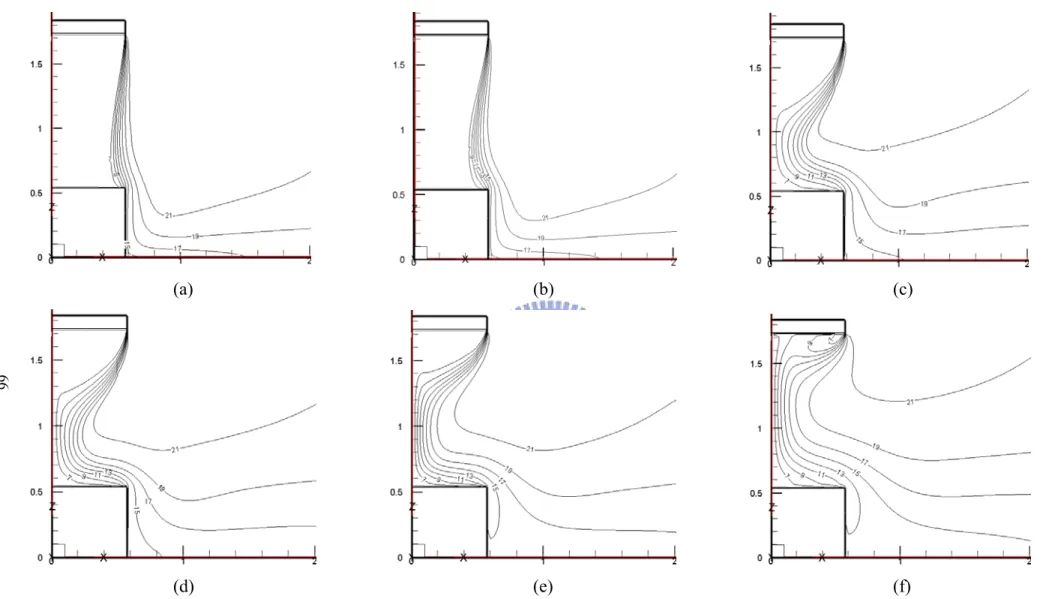
(ΔT = 20℃), and N = 6.37 × 10-2for Reb = (a) 9,548 (Vj = 1.5 m/s), (b) 8,275 ( Vj = 1.3 m/s), (c) 6,365 ( Vj = 1.0 m/s), (d) 5,092 ( Vj = 0.8 m/s), (e) 3,183 ( Vj = 0.5 m/s) and (f) 1,910 ( Vj = 0.3 m/s).--- 62 Fig. 4.5 Isotherms in the cavity for steady cavity flow for bj = 0.1 m, Grt = 4.61 ×

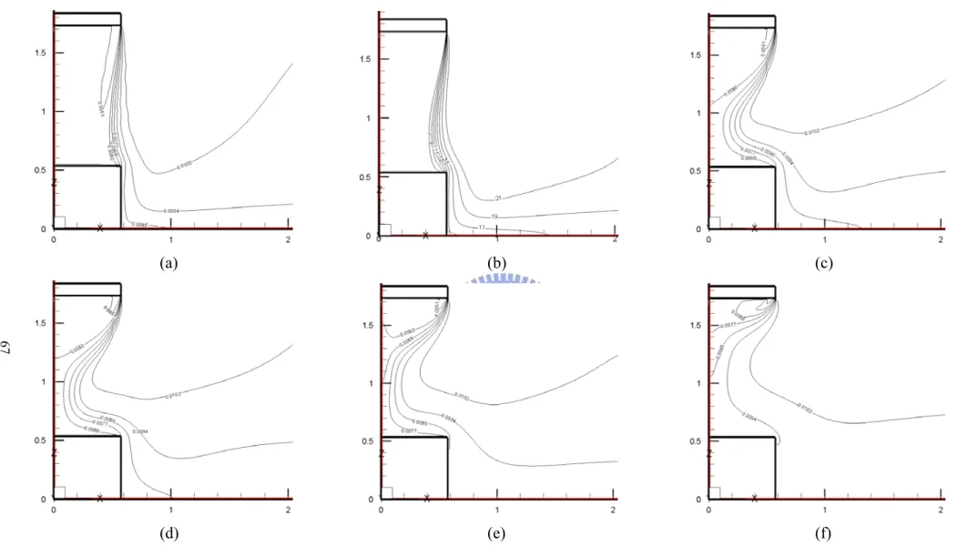
109 (ΔT = 20℃), and N = 6.37 × 10-2for Reb = (a) 9,548 (Vj = 1.5 m/s), (b) 8,275 ( Vj = 1.3 m/s), (c) 6,365 ( Vj = 1.0 m/s), (d) 5,092 ( Vj = 0.8 m/s), (e) 3,183 ( Vj = 0.5 m/s) and (f) 1,910 ( Vj = 0.3 m/s).--- 63 Fig. 4.6 Iso-concentration lines in the cavity for steady cavity flow for bj = 0.1 m,

Grt = 4.61 × 109 (ΔT = 20℃), and N = 6.37 × 10-2 for Reb = (a) 9,548 (Vj = 1.5 m/s), (b) 8,275 ( Vj = 1.3 m/s), (c) 6,365 ( Vj = 1.0 m/s), (d) 5,092 ( Vj = 0.8 m/s), (e) 3,183 ( Vj = 0.5 m/s) and (f) 1,910 ( Vj = 0.3 m/s). --- 64 Fig. 4.7 Velocity vector maps for steady cavity flow for bj = 0.07 m, Grt = 4.61 ×

109 (ΔT = 20℃), and N = 6.37 × 10-2 for Reb = (a) 9,548 ( Vj = 2.143 m/s), (b) 8,275 ( Vj = 1.857 m/s), (c) 6,365 ( Vj = 1.428 m/s), (d) 5,092 ( Vj = 1.143 m/s), (e) 3,183 ( Vj = 0.714 m/s) and (f) 1,910 ( Vj = 0.428 m/s).-- 65

(17)

Fig. 4.8 Isotherms in the cavity for steady cavity flow for b = 0.07 m, Grt = 4.61 × 109 (ΔT = 20℃), and N = 6.37 × 10-2 for Reb = (a) 9,548 ( Vj = 2.143 m/s), (b) 8,275 ( Vj = 1.857 m/s), (c) 6,365 ( Vj = 1.428 m/s), (d) 5,092 ( Vj = 1.143 m/s), (e) 3,183 ( Vj = 0.714 m/s) and (f) 1,910 ( Vj = 0.428 m/s).-- 66 Fig. 4.9 Iso-concentration lines in the cavity for steady cavity flow for b = 0.07 m,

Grt = 4.61 × 109 (ΔT = 20℃), and N = 6.37 × 10-2 for Reb = (a) 9,548 ( Vj = 2.143 m/s), (b) 8,275 ( Vj = 1.857 m/s), (c) 6,365 ( Vj = 1.428 m/s), (d) 5,092 ( Vj = 1.143 m/s), (e) 3,183 ( Vj = 0.714 m/s) and (f) 1,910 ( Vj = 0.428 m/s). --- 67 Fig. 4.10 Velocity vector maps for steady cavity flow for bj = 0.05 m, Grt = 4.61 ×

109 (ΔT = 20℃), and N = 6.37 × 10-2 for Reb = (a) 9,548 ( Vj = 3 m/s), (b) 8,275 ( Vj = 2.6 m/s), (c) 6,365 ( Vj = 2.0 m/s), (d) 5,092 ( Vj = 1.6 m/s), (e) 3,183 ( Vj = 1.0 m/s) and (f) 1,910 ( Vj = 0.6 m/s).--- 68 Fig. 4.11 Isotherms in the cavity for steady cavity flow for bj = 0.05 m, Grt = 4.61 ×

109 (ΔT = 20℃), and N = 6.37 × 10-2 for Reb = (a) 9,548 ( Vj = 3 m/s), (b) 8,275 ( Vj = 2.6 m/s), (c) 6,365 ( Vj = 2.0 m/s), (d) 5,092 ( Vj = 1.6 m/s), (e) 3,183 ( Vj = 1.0 m/s) and (f) 1,910 ( Vj = 0.6 m/s).--- 69 Fig. 4.12 Iso-concentration lines in the cavity for steady cavity flow for bj = 0.05 m,

Grt = 4.61 × 109 (ΔT = 20℃), and N = 6.37 × 10-2 for Reb = (a) 9,548 ( Vj = 3 m/s), (b) 8,275 ( Vj = 2.6 m/s), (c) 6,365 ( Vj = 2.0 m/s), (d) 5,092 ( Vj = 1.6 m/s), (e) 3,183 ( Vj = 1.0 m/s) and (f) 1,910 ( Vj = 0.6 m/s). --- 70 Fig. 4.13 Velocity vector maps for steady cavity flow for bj = 0.1 m, Grt = 4.61 × 109

(ΔT = 20℃), and N = 6.37 × 10-2 with a jet inclined angle of 5。

for Reb = (a) 9,548 (Vj = 1.5 m/s), (b) 8,275 ( Vj = 1.3 m/s), (c) 6,365 ( Vj = 1.0 m/s), (d) 5,092 ( Vj = 0.8 m/s), (e) 3,183 ( Vj = 0.5 m/s) and (f) 1,910 ( Vj = 0.3 m/s). --- 71

(18)

Fig. 4.14 Isotherms for steady cavity flow for bj = 0.1 m, Grt = 4.61 × 109 (ΔT = 20 ℃), and N = 6.37 × 10-2 with a jet inclined angle of 5。

for Reb = (a) 9,548 (Vj = 1.5 m/s), (b) 8,275 ( Vj = 1.3 m/s), (c) 6,365 ( Vj = 1.0 m/s), (d) 5,092 ( Vj = 0.8 m/s), (e) 3,183 ( Vj = 0.5 m/s) and (f) 1,910 ( Vj = 0.3 m/s). --- 72 Fig. 4.15 Iso-concentration lines for steady cavity flow for bj = 0.1 m, Grt = 4.61 ×

109 (ΔT = 20℃), and N = 6.37 × 10-2 with a jet inclined angle of 5。

for Reb = (a) 9,548 (Vj = 1.5 m/s), (b) 8,275 ( Vj = 1.3 m/s), (c) 6,365 ( Vj = 1.0 m/s), (d) 5,092 ( Vj = 0.8 m/s), (e) 3,183 ( Vj = 0.5 m/s) and (f) 1,910 ( Vj = 0.3 m/s). --- 73 Fig. 4.16 Velocity vector maps for steady cavity flow for bj = 0.1 m, Grt = 4.61 × 109

for Reb = (a) 9,548 (Vj = 1.5 m/s), (b) 8,275 ( Vj = 1.3 m/s), (c) 6,365 ( Vj = 1.0 m/s), (d) 5,092 ( Vj = 0.8 m/s), (e) 3,183 ( Vj = 0.5 m/s) and (f) 1,910 ( Vj = 0.3 m/s).--- 74 Fig. 4.17 Isotherms for steady cavity flow for bj = 0.1 m, Grt = 4.61 × 109 (ΔT = 20

℃), and N = 6.37 × 10-2 with a jet inclined angle of 15。

for Reb = (a) 9,548 (Vj = 1.5 m/s), (b) 8,275 ( Vj = 1.3 m/s), (c) 6,365 ( Vj = 1.0 m/s), (d) 5,092 ( Vj = 0.8 m/s), (e) 3,183 ( Vj = 0.5 m/s) and (f) 1,910 ( Vj = 0.3 m/s). --- 76 Fig. 4.19 Velocity vector maps for steady cavity flow for bj = 0.1 m, Grt = 4.61 × 109

for Reb = (a) 9,548 (Vj = 1.5 m/s), (b) 8,275 ( Vj = 1.3 m/s), (c) 6,365 ( Vj = 1.0 m/s),

(19)

(d) 5,092 ( Vj = 0.8 m/s), (e) 3,183 ( Vj = 0.5 m/s) and (f) 1,910 ( Vj = 0.3 m/s).--- 77 Fig. 4.20 Isotherms for steady cavity flow for bj = 0.1 m, Grt = 4.61 × 109 (ΔT = 20

for Reb = (a) 9,548 (Vj = 1.5 m/s), (b) 8,275 ( Vj = 1.3 m/s), (c) 6,365 ( Vj = 1.0 m/s), (d) 5,092 ( Vj = 0.8 m/s), (e) 3,183 ( Vj = 0.5 m/s) and (f) 1,910 ( Vj = 0.3 m/s). --- 79 Fig. 4.22 Velocity vector maps for steady cavity flow for bj = 0.07 m, Grt = 4.61 ×

for Reb = (a) 9,548 ( Vj = 2.143 m/s), (b) 8,275 ( Vj = 1.857 m/s), (c) 6,365 ( Vj = 1.428 m/s), (d) 5,092 ( Vj = 1.143 m/s), (e) 3,183 ( Vj = 0.714 m/s) and (f) 1,910 ( Vj = 0.428 m/s). --- 80 Fig. 4.23 Isotherms for steady cavity flow for bj = 0.07 m, Grt = 4.61 × 109 (ΔT = 20

for Reb = (a) 9,548 ( Vj = 2.143 m/s), (b) 6,365 ( Vj = 1.428 m/s), (c) 5,092 ( Vj = 1.143 m/s), (d) 3,183 ( Vj = 0.714 m/s) and (e) 1,910 ( Vj = 0.428 m/s). --- 81 Fig. 4.24 Iso-concentration lines for steady cavity flow for bj = 0.07 m, Grt = 4.61 ×

for Reb = (a) 9,548 ( Vj = 2.143 m/s), (b) 6,365 ( Vj = 1.428 m/s), (c) 5,092 ( Vj = 1.143 m/s), (d) 3,183 ( Vj = 0.714 m/s) and (e) 1,910 ( Vj = 0.428 m/s)-- 82 Fig. 4.25 Velocity vector maps for steady cavity flow for bj = 0.07 m, Grt = 4.61 ×

(20)

= (a) 9,548 ( Vj = 2.142 m/s), (b) 8,275 ( Vj = 1.857 m/s), (c) 6,365 ( Vj = 1.428 m/s), (d) 5,092 ( Vj = 1.142 m/s), (e) 3,183 ( Vj = 0.714 m/s) and (f) 1,910 ( Vj = 0.428 m/s). --- 83 Fig. 4.26 Isotherms for steady cavity flow for bj = 0.07 m, Grt = 4.61 × 109 (ΔT = 20

for Reb = (a) 9,548 ( Vj = 2.142 m/s), (b) 8,275 ( Vj = 1.857 m/s), (c) 6,365 ( Vj = 1.428 m/s), (d) 5,092 ( Vj = 1.142 m/s), (e) 3,183 ( Vj = 0.714 m/s) and (f) 1,910 ( Vj = 0.428 m/s). --- 84 Fig. 4.27 Iso-concentration lines for steady cavity flow for bj = 0.07 m, Grt = 4.61 ×

for Reb = (a) 9,548 ( Vj = 2.142 m/s), (b) 8,275 ( Vj = 1.857 m/s), (c) 6,365 ( Vj = 1.428 m/s), (d) 5,092 ( Vj = 1.142 m/s), (e) 3,183 ( Vj = 0.714 m/s) and (f) 1,910 ( Vj = 0.428 m/s). --- 85 Fig. 4.28 Velocity vector maps for steady cavity flow for bj = 0.07 m, Grt = 4.61 ×

for Reb = (a) 9,548 ( Vj = 2.142 m/s), (b) 8,275 ( Vj = 1.857 m/s), (c) 6,365 ( Vj = 1.428 m/s), (d) 5,092 ( Vj = 1.142 m/s), (e) 3,183 ( Vj = 0.714 m/s) and (f) 1,910 ( Vj = 0.428 m/s). --- 86 Fig. 4.29 Isotherms for steady cavity flow for bj = 0.07 m, Grt = 4.61 × 109 (ΔT = 20

for Reb = (a) 9,548 ( Vj = 2.142 m/s), (b) 8,275 ( Vj = 1.857 m/s), (c) 6,365 ( Vj = 1.428 m/s), (d) 5,092 ( Vj = 1.142 m/s), (e) 3,183 ( Vj = 0.714 m/s) and (f) 1,910 ( Vj = 0.428 m/s). --- 87 Fig. 4.30 Iso-concentration lines for steady cavity flow for bj = 0.07 m, Grt = 4.61 ×

for Reb = (a) 9,548 ( Vj = 2.142 m/s), (b) 8,275 ( Vj = 1.857 m/s), (c) 6,365 ( Vj

(21)

= 1.428 m/s), (d) 5,092 ( Vj = 1.142 m/s), (e) 3,183 ( Vj = 0.714 m/s) and (f) 1,910 ( Vj = 0.428 m/s). --- 88 Fig. 4.31 Velocity vector maps for steady cavity flow for bj = 0.05 m, Grt = 4.61 ×

for Reb = (a) 9,548 ( Vj = 3 m/s), (b) 8,275 ( Vj = 2.6 m/s), (c) 6,365 ( Vj = 2.0 m/s), (d) 5,092 ( Vj = 1.6 m/s), (e) 3,183 ( Vj = 1.0 m/s) and (f) 1,910 ( Vj = 0.6 m/s).--- 89 Fig. 4.32 Isotherms for steady cavity flow for bj = 0.05 m, Grt = 4.61 × 109 (ΔT = 20

for Reb = (a) 9,548 ( Vj = 3 m/s), (b) 8,275 ( Vj = 2.6 m/s), (c) 6,365 ( Vj = 2.0 m/s), (d) 5,092 ( Vj = 1.6 m/s), (e) 3,183 ( Vj = 1.0 m/s) and (f) 1,910 ( Vj = 0.6 m/s). --- 90 Fig. 4.33 Iso-concentration lines for steady cavity flow for bj = 0.05 m, Grt = 4.61 ×

for Reb = (a) 9,548 ( Vj = 3 m/s), (b) 8,275 ( Vj = 2.6 m/s), (c) 6,365 ( Vj = 2.0 m/s), (d) 5,092 ( Vj = 1.6 m/s), (e) 3,183 ( Vj = 1.0 m/s) and (f) 1,910 ( Vj = 0.6 m/s).--- 91 Fig. 4.34 Velocity vector maps for steady cavity flow for bj = 0.05 m, Grt = 4.61 ×

(22)

for Reb = (a) 9,548 ( Vj = 3 m/s), (b) 8,275 ( Vj = 2.6 m/s), (c) 6,365 ( Vj = 2.0 m/s), (d) 5,092 ( Vj = 1.6 m/s), (e) 3,183 ( Vj = 1.0 m/s) and (f) 1,910 ( Vj = 0.6 m/s). --- 94 Fig. 4.37 Velocity vector maps for steady cavity flow for bj = 0.05 m, Grt = 4.61 ×

for Reb = (a) 9,548 ( Vj = 3 m/s), (b) 8,275 ( Vj = 2.6 m/s), (c) 6,365 ( Vj = 2.0 m/s), (d) 5,092 ( Vj = 1.6 m/s), (e) 3,183 ( Vj = 1.0 m/s) and (f) 1,910 ( Vj = 0.6 m/s). --- 97 Fig. 4.40 Velocity vector maps for steady cavity flow for a double air curtain design

with bi = 0.03 m, bo = 0.07 m, Grt = 4.61 × 109 (ΔT = 20℃), and N = 6.37 × 10-2 for Reci = 1,910 and Reco = (a) 1,910, (b) 3,183, (c) 5,092, (d) 6,365 and (e) 7,638. --- 98 Fig. 4.41 Isotherms for steady cavity flow for a double air curtain design with bi =

0.03 m, bo = 0.07 m, Grt = 4.61 × 109 (ΔT = 20℃), and N = 6.37 × 10-2 for Reci = 1,910 and Reco = (a) 1,910, (b) 3,183, (c) 5,092, (d) 6,365 and (e) 7,638. --- 99

(23)

Fig. 4.42 Iso-concentration lines for steady cavity flow for a double air curtain design with bi = 0.03 m, bo = 0.07 m, Grt = 4.61 × 109 (ΔT = 20℃), and N = 6.37 × 10-2 for Reci = 1,910 and Reco = (a) 1,910, (b) 3,183, (c) 5,092, (d) 6,365 and (e) 7,638.---100 Fig. 4.43 Velocity vector maps for steady cavity flow for a double air curtain design

with bi = 0.03 m, bo = 0.07 m, Grt = 4.61 × 109 (ΔT = 20℃), and N = 6.37 × 10-2 for Reci = 3,183 and Reco = (a) 1,910, (b) 3,183, (c) 5,092, and (d) 6,365. ---101 Fig. 4.44 Isotherms for steady cavity flow for a double air curtain design with bi =

0.03 m, bo = 0.07 m, Grt = 4.61 × 109 (ΔT = 20℃), and N = 6.37 × 10-2 for Reci = 3,183 and Reco = (a) 1,910, (b) 3,183, (c) 5,092, and (d) 6,365. --102 Fig. 4.45 Iso-concentration lines for steady cavity flow for a double air curtain

design with bi = 0.03 m, bo = 0.07 m, Grt = 4.61 × 109 (ΔT = 20℃), and N = 6.37 × 10-2 for Reci = 3,183 and Reco = (a) 1,910, (b) 3,183, (c) 5,092, and (d) 6,365. ---103 Fig. 4.46 Velocity vector maps for steady cavity flow for a double air curtain design

with bi = 0.03 m, bo = 0.07 m, Grt = 4.61 × 109 (ΔT = 20℃), and N = 6.37 × 10-2 for (a) Reci = 1,910 and Reco = 7,638, (b) Reci = 3,183 and Reco = 6,365, (c) Reci = 5,092 and Reco = 4,456, (d) Reci = 6,365 and Reco = 3,183, (e) Reci = 7,638 and Reco = 1,910. ---104 Fig. 4.47 Isotherms for steady cavity flow for a double air curtain design with bi =

0.03 m, bo = 0.07 m, Grt = 4.61 × 109 (ΔT = 20℃), and N = 6.37 × 10-2 for (a) Reci = 1,910 and Reco = 7,638, (b) Reci = 3,183 and Reco = 6,365, (c) Reci = 5,092 and Reco = 4,456, (d) Reci = 6,365 and Reco = 3,183, (e) Reci = 7,638 and Reco = 1,910. ---105 Fig. 4.48 Iso-concentration lines for steady cavity flow for a double air curtain

(24)

design with bi = 0.03 m, bo = 0.07 m, Grt = 4.61 × 109 (ΔT = 20℃), and N = 6.37 × 10-2 for (a) Reci = 1,910 and Reco = 7,638, (b) Reci = 3,183 and Reco = 6,365, (c) Reci = 5,092 and Reco = 4,456, (d) Reci = 6,365 and Reco = 3,183, (e) Reci = 7,638 and Reco = 1,910. ---106 Fig. 4.49 Velocity vector maps for steady cavity flow for a double air curtain design

with bi = 0.05 m, bo = 0.05 m, Grt = 4.61 × 109 (ΔT = 20℃), and N = 6.37 × 10-2 for Reci = 1,910 and Reco = (a) 1,910, (b) 3,183, (c) 5,092, (d) 6,365 and (e) 7,638. ---107 Fig. 4.50 Isotherms for steady cavity flow for a double air curtain design with bi =

0.05 m, bo = 0.05 m, Grt = 4.61 × 109 (ΔT = 20℃), and N = 6.37 × 10-2 for Reci = 1,910 and Reco = (a) 1,910, (b) 3,183, (c) 5,092, (d) 6,365 and (e) 7,638. ---108 Fig. 4.51 Iso-concentration lines for steady cavity flow for a double air curtain

design with bi = 0.05 m, bo = 0.05 m, Grt = 4.61 × 109 (ΔT = 20℃), and N = 6.37 × 10-2 for Reci = 1,910 and Reco = (a) 1,910, (b) 3,183, (c) 5,092, (d) 6,365 and (e) 7,638.---109 Fig. 4.52 Velocity vector maps for steady cavity flow for a double air curtain design

0.05 m, bo = 0.05 m, Grt = 4.61 × 109 (ΔT = 20℃), and N = 6.37 × 10-2 for Reci = 3,183 and Reco = (a) 1,910, (b) 3,183, (c) 5,092, and (d) 6,365. -- 111 Fig. 4.54 Iso-concentration lines for steady cavity flow for a double air curtain

design with bi = 0.05 m, bo = 0.05 m, Grt = 4.61 × 109 (ΔT = 20℃), and N = 6.37 × 10-2 for Reci = 3,183 and Reco = (a) 1,910, (b) 3,183, (c) 5,092, and

(25)

(d) 6,365. ---112 Fig. 4.55 Velocity vector maps for steady cavity flow for a double air curtain design

(26)

= 6.37 × 10-2 for Reci = 1,910 and Reco = (a) 1,910, (b) 3,183, (c) 5,092, (d) 6,365 and (e) 7,638.---118 Fig. 4.61 Velocity vector maps for steady cavity flow for a double air curtain design

design with bi = 0.07 m, bo = 0.03 m, Grt = 4.61 × 109 (ΔT = 20℃), and N = 6.37 × 10-2 for (a) Reci = 1,910 and Reco = 7,638, (b) Reci = 3,183 and

(27)

Reco = 6,365, (c) Reci = 5,092 and Reco = 4,456, (d) Reci = 6,365 and Reco = 3,183, (e) Reci = 7,638 and Reco = 1,910. ---124 Fig. 4.67 Velocity vector maps for steady cavity flow for a double air curtain design

(28)

design with bi = 0.09 m, bo = 0.03 m, Grt = 4.61 × 109 (ΔT = 20℃), and N = 6.37 × 10-2 for Reci = 1,910 and Reco = (a) 1,910, (b) 3,183, (c) 5,092, (d) 6,365 and (e) 7,638.---136

(29)

Fig. 4.79 Velocity vector maps for steady cavity flow for a double air curtain design with bi = 0.09 m, bo = 0.03 m, Grt = 4.61 × 109 (ΔT = 20℃), and N = 6.37 × 10-2 for Reci = 3,183 and Reco = (a) 1,910, (b) 3,183, (c) 5,092, and (d) 6,365. ---137 Fig. 4.80 Isotherms for steady cavity flow for a double air curtain design with bi =

design with bi = 0.09 m, bo = 0.03 m, Grt = 4.61 × 109 (ΔT = 20℃), and N = 6.37 × 10-2 for (a) Reci = 1,910 and Reco = 7,638, (b) Reci = 3,183 and Reco = 6,365, (c) Reci = 5,092 and Reco = 4,456, (d) Reci = 6,365 and Reco = 3,183, (e) Reci = 7,638 and Reco = 1,910. ---142

(30)

Fig. 4.85 Velocity vector maps for steady cavity flow for a double air curtain design with bi = 0.05 m, bo = 0.07 m, Grt = 4.61 × 109 (ΔT = 20℃), and N = 6.37 × 10-2 for Reci = 1,910 and Reco = (a) 1,910, (b) 3,183, (c) 5,092, (d) 6,365 and (e) 7,638. ---143 Fig. 4.86 Isotherms for steady cavity flow for a double air curtain design with bi =

with bi = 0.05 m, bo = 0.07 m, Grt = 4.61 × 109 (ΔT = 20℃), and N = 6.37 × 10-2 for (a) Reci = 1,910 and Reco = 7,638, (b) Reci = 3,183 and Reco =

(31)

6,365, (c) Reci = 5,092 and Reco = 4,456, (d) Reci = 6,365 and Reco = 3,183, (e) Reci = 7,638 and Reco = 1,910. ---149 Fig. 4.92 Isotherms for steady cavity flow for a double air curtain design with bi =

(32)

× 10-2 for Reci = 3,183 and Reco = (a) 1,910, (b) 3,183, (c) 5,092, and (d) 6,365. ---155 Fig. 4.98 Isotherms for steady cavity flow for a double air curtain design with bi =

(33)

× 10-2 for Reci = 1,910 and Reco = (a) 1,910, (b) 3,183, (c) 5,092, (d) 6,365 and (e) 7,638. ---161 Fig. 4.104 Isotherms for steady cavity flow for a double air curtain design with bi =

with bi = 0.03 m, bo = 0.04 m, Grt = 4.61 × 109 (ΔT = 20℃), and N = 6.37 × 10-2 for (a) Reci = 1,910 and Reco = 7,638, (b) Reci = 3,183 and Reco = 6,365, (c) Reci = 5,092 and Reco = 4,456, (d) Reci = 6,365 and Reco = 3,183, (e) Reci = 7,638 and Reco = 1,910. ---167

(34)

Fig. 4.110 Isotherms for steady cavity flow for a double air curtain design with bi = 0.03 m, bo = 0.04 m, Grt = 4.61 × 109 (ΔT = 20℃), and N = 6.37 × 10-2 for (a) Reci = 1,910 and Reco = 7,638, (b) Reci = 3,183 and Reco = 6,365, (c) Reci = 5,092 and Reco = 4,456, (d) Reci = 6,365 and Reco = 3,183, (e) Reci = 7,638 and Reco = 1,910. ---168 Fig. 4.111 Iso-concentration lines for steady cavity flow for a double air curtain

with bi = 0.04 m, bo = 0.03 m, Grt = 4.61 × 109 (ΔT = 20℃), and N = 6.37 × 10-2 for Reci = 3,183 and Reco = (a) 1,910, (b) 3,183, (c) 5,092, and (d) 6,365. ---173

(35)

Fig. 4.116 Isotherms for steady cavity flow for a double air curtain design with bi = 0.04 m, bo = 0.03 m, Grt = 4.61 × 109 (ΔT = 20℃), and N = 6.37 × 10-2 for Reci = 3,183 and Reco = (a) 1,910, (b) 3,183, (c) 5,092, and (d) 6,365. --174 Fig. 4.117 Iso-concentration lines for steady cavity flow for a double air curtain

with bi = 0.05 m, and bo = 0.05 m, Grt = 4.61 × 109 (ΔT = 20℃), and N = 6.37 × 10-2 with a outer curtain inclined angle of 25。

for Reci = 1,910 and Reco = (a) 1,910, (b) 3,183, (c) 5,092, (d) 6,365 and (e) 7,638. ---179

(36)

Fig. 4.122 Isotherms for steady cavity flow for a double air curtain design with bi = 0.05 m, and bo = 0.05 m, Grt = 4.61 × 109 (ΔT = 20℃), and N = 6.37 × 10-2 with a outer curtain inclined angle of 25。

for Reci = 1,910 and Reco = (a) 1,910, (b) 3,183, (c) 5,092, (d) 6,365 and (e) 7,638.---180 Fig. 4.123 Iso-concentration lines for steady cavity flow for a double air curtain

design with bi = 0.05 m, and bo = 0.05 m, Grt = 4.61 × 109 (ΔT = 20℃), and N = 6.37 × 10-2 with a outer curtain inclined angle of 25。

for Reci = 3,183 and Reco = (a) 1,910, (b) 3,183, (c) 5,092, (d) 6,365 and (e) 7,638. ----181 Fig. 4.124 Velocity vector maps for steady cavity flow for a double air curtain design

for Reci = 3,183 and Reco = (a) 1,910, (b) 3,183, (c) 5,092, and (d) 6,365.---182 Fig. 4.125 Isotherms for steady cavity flow for a double air curtain design with bi =

0.05 m, and bo = 0.05 m, Grt = 4.61 × 109 (ΔT = 20℃), and N = 6.37 × 10-2 with a outer curtain inclined angle of 25。

for Reci = 3,183 and Reco = (a) 1,910, (b) 3,183, (c) 5,092, and (d) 6,365. ---183 Fig. 4.126 Iso-concentration lines for steady cavity flow for a double air curtain

for Reci = 3,183 and Reco = (a) 1,910, (b) 3,183, (c) 5,092, and (d) 6,365.---184 Fig. 4.127 Velocity vector maps for steady cavity flow for a double air curtain design

for (a) Reci = 1,910 and Reco = 7,638, (b) Reci = 3,183 and Reco = 6,365, (c) Reci = 5,092 and Reco = 4,456, (d) Reci = 6,365 and Reco = 3,183, (e) Reci = 7,638 and Reco = 1,910. ---185

(37)

Fig. 4.128 Isotherms for steady cavity flow for a double air curtain design with bi = 0.05 m, and bo = 0.05 m, Grt = 4.61 × 109 (ΔT = 20℃), and N = 6.37 × 10-2 with a outer curtain inclined angle of 25。

for (a) Reci = 1,910 and Reco = 7,638, (b) Reci = 3,183 and Reco = 6,365, (c) Reci = 5,092 and Reco = 4,456, (d) Reci = 6,365 and Reco = 3,183, (e) Reci = 7,638 and Reco = 1,910. ---186 Fig. 4.129 Iso-concentration lines for steady cavity flow for a double air curtain

for (a) Reci = 1,910 and Reco = 7,638, (b) Reci = 3,183 and Reco = 6,365, (c) Reci = 5,092 and Reco = 4,456, (d) Reci = 6,365 and Reco = 3,183, (e) Reci = 7,638 and Reco = 1,910. ---187 Fig. 4.130 Schematic diagram of an open vertical cavity with back panel perforation.

---188 Fig. 4.131 Velocity vector maps for steady cavity flow for a single air curtain design

with perforation density of 35% for bj = 0.1 m, Grt = 4.61 × 109 (ΔT = 20 ℃), and N = 6.37 × 10-2 for Rep = 1,910 and Reb = (a) 1,910, (b) 3,183, (c) 5,092, (d) 6,365, and (e) 9,548. ---189 Fig. 4.132 Isotherms for steady cavity flow for a single air curtain design with

perforation density of 35% for bj = 0.1 m, Grt = 4.61 × 109 (ΔT = 20℃), and N = 6.37 × 10-2 for Rep = 1,910 and Reb = (a) 1,910, (b) 3,183, (c) 5,092, (d) 6,365, and (e) 9,548. ---190 Fig. 4.133 Iso-concentration lines for steady cavity flow for a single air curtain

design with perforation density of 35% for bj = 0.1 m, Grt = 4.61 × 109 (ΔT = 20℃), and N = 6.37 × 10-2 for Rep = 1,910 and Reb = (a) 1,910, (b) 3,183, (c) 5,092, (d) 6,365, and (e) 9,548. ---191 Fig. 4.134 Velocity vector maps for steady cavity flow for a single air curtain design

(38)

perforation density of 35% for bj = 0.1 m, Grt = 4.61 × 109 (ΔT = 20℃), and N = 6.37 × 10-2 for Rep = 3,183 and Reb = (a) 1,910 (b) 3,183, (c) 5,092, (d) 6,365, and (e) 9,548.---193 Fig. 4.136 Iso-concentration lines for steady cavity flow for a single air curtain

with perforation density of 25% for bj = 0.1 m, Grt = 4.61 × 109 (ΔT = 20 ℃), and N = 6.37 × 10-2 for Rep = 1,910 and Reb = (a) 1,910, (b) 3,183, (c)

(39)

5,092, (d) 6,365, and (e) 9,548. ---198 Fig. 4.141 Isotherms for steady cavity flow for a single air curtain design with

(40)

perforation density of 15% for bj = 0.1 m, Grt = 4.61 × 109 (ΔT = 20℃), and N = 6.37 × 10-2 for Rep = 3,183 and Reb = (a) 1,910 (b) 3,183, (c) 5,092,

(41)

(d) 6,365, and (e) 9,548.---211 Fig. 4.154 Iso-concentration lines for steady cavity flow for a single air curtain

design with perforation density of 15% for bj = 0.1 m, Grt = 4.61 × 109 (ΔT = 20℃), and N = 6.37 × 10-2 for Rep = 5,092 and Reb = (a) 1,910, (b) 3,183, (c) 5,092, (d) 6,365, and (e) 9,548. ---215

(42)

LIST OF TABLES

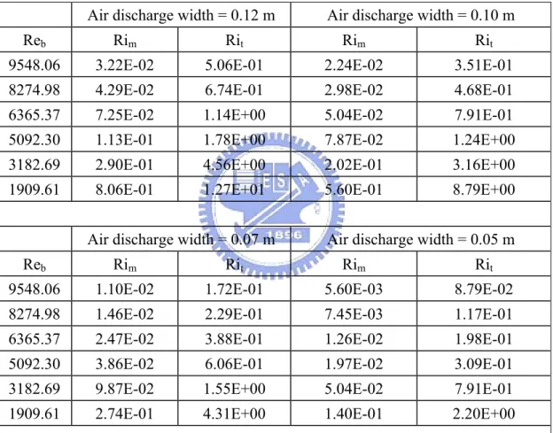
Table 4.1 Variations of Richardson numbers with the jet Reynolds number. --- 57 Table 4.2 Entrainment factors for selected cases with a single air curtain design. -- 58

(43)

NOMENCLATURE

A Ratio of the discharge to return grille distance to the discharge width / j

A=H b

bj Jet width at the air curtain discharge (m)

B Upper and bottom plates of the cavity, Bb(bottom) and Bc(ceiling) cp Specific heat at constant pressure, J/(kg Ki )

D Solutal diffusivity, m2/s

dp Back panel perforation density g Gravitational acceleration (m/s2) Gr Grashof number, 3 2 3 2 1 , t t m m Gr =gβΔTH ν Gr =gβ Δw H ν

Gr/ReH2 Ratio of thermal buoyancy-to-inertia force, Richardson number H Distance between the discharge grilles to return grilles (m) k Thermal conductivity

K Instantaneous value of turbulence kinetic energy, u u_i′ ′_i/ 2 (m2/s2) K Average value of turbulence kinetic energy, u u_i′ ′_i/ 2 (m2/s2)

Le Lewis number, Le=ν α/

Ma, Mv Molecular weights of air and water vapor, respectively N Buoyancy ratio, βm

(

w₁a −wj

) (

/βt Tamb−Tj

)

P Non-dimensional pressure pamb Pressure of the ambient, 101325 Pa pm Motion pressure

Pr Prandtl number, Pr=ν α/ ,Pr_t =μ_tC_p/k_t

(44)

Ra _{Rayleigh numbers,} 3 3 1 , t m Ra =gβΔTH αν Ra =gβΔw H αν Re _{Reynolds numbers,} _{/ ,} _{/ ,} _/ b j j H j p p p Re =V b ν Re =V H ν Re =V Hd ν Ri _{Richardson number,} 2 _, 2 t t H m t H Ri =Gr Re Ri =Gr Re Sc Schmidt numbers,Sc=ν / ,D Sc_t =μ ρ_t/ D T Temperature

TC Temperature of the inner cold plate (℃) Tj Temperature of air at the discharge grille (℃) Tamb Temperature of the ambient surrounding (℃) t , τ Dimensional (sec.) and dimensionless times

u, w _{Dimensional velocity components} U, W Dimensionless velocity components

j

V Uniform velocity of the air jet at the discharge grille inlet (m/s)

p

V Average air speed at perforations (m/s)

w1 Mass fraction of moisture

w1a Mass fraction of moisture of the ambient w1j Mass fraction of moisture of the air discharge x,z Dimensional Cartesian coordinates

Y+ Non-dimensional distance from wall in wall coordinates X,Z Dimensionless Cartesian coordinates, x H z H / , /

Greek

symbols

α Thermal diffusivity of the mixture (cm2/s) αe Thermal entrainment factor

(45)

ΔT Temperature difference between the ambient and the air discharge (℃)

Θ Nondimensional temperature,

(

T −TC

)

/

(

Tamb−TC

)

t

β Thermal expansion coefficient, (1/T0)

m

β Concentration expansion coefficient, (Ma/Mv-1) ν Kinematic viscosity of the mixture (m2/s)

ρ Mass density of the mixture

ε Turbulence dissipation rate, N/(sm2)

φ Relative humidity ρ

γ Ratio of density, ρ ρ/ ₀ μ

γ Ratio of dynamic viscosity, μ μ/ ₀

cp

γ Ratio of specific heat at constant pressure, Cp/C p₀ k

λ Ratio of thermal conductivity, k k / ₀

D

λ Ratio of mass diffusivity, D D / ₀

Subscripts

0 At reference condition

a of air

amb at ambient condition j At air curtain discharge v of water vapor

b Parameters based on air discharge width

H Parameters based on distance between air discharge to return grilles i Inner curtain of double curtain design

o Outer curtain of double curtain design p of back panel

(46)

(47)

CHAPTER 1 INTRODUCTION

1.1 Motivation

In view of the recent significant improvement in the standard of living, refrigerated display cases are extensively used in today’s supermarkets and grocery stores. To save precious floor-space and provide a large selling area, vertical display cabinets are the better choice than the horizontal ones [1]. Moreover, to attract consumers and hence increase sales, manufacturers developed open type display cases, as schematically shown in Fig. 1.1, with no obstacle between the products and customers [1-4]. In these display cases a cold air curtain is often used to produce an artificial barrier between the outside warm air in the ambient and inside cold air in the cabinets. The air curtain is essentially a two-dimensional cool air jet. Usually the air curtain is supplied from the top of a display case through a discharge honeycomb, flows over the open surface of the cabinet, and finally reaches a return air grille at the case bottom. In reality, an open display case is operated in a store environment and it exchanges heat and moisture with the surrounding air in the store. Besides, the outside warm and moist air can be entrained into the display case by the air curtain, which in turn can substantially lower the performance of the case. Note that the entrained warm and moist air into the cabinet becomes sensible and latent energy loads to the unit since it needs to be cooled and the moisture in it needs to be removed. Therefore a detailed understanding of the heat and mass transfer processes in open refrigerated display cases are needed to improve the performance of the systems. Especially, how the momentum, energy and moisture transports in the

(48)

cabinets are affected by the moist air entrained into the flow and buoyancy forces in the flow requires an in-depth investigation.

1.2 Literature Review

The literature relevant to the present study is reviewed in the following.

1.2.1 Cooling loads

The total cooling loads of a refrigerated display cabinet consists of sensible and latent components. The sensible portion includes heat conduction through physical envelopes of the cabinet, thermal radiation from the ambient to the cabinet, sensible infiltration, and heat gains from fan motors, anti-sweat heater and defrost. The latent portion comes from the entrainment of the moisture in the ambient into the cabinet through the air curtains. Ge and Tassou [5] used an implicit numerical method to simulate flow and heat transfer in a vertical display case and developed an correlation for the total heat transfer across an air curtain in terms of the ambient air enthalpy, initial dry-bulb temperature of air jet, temperature difference between the air inside the cabinet and injected air, and some air curtain properties such as the jet initial velocity, jet mass flow rate and jet length. Jet thickness is not directly included, but has some relationship with the jet velocity and mass flow rate. They also proposed a correlation for the return air temperature based on air temperature at the injection grille and ambient and on the air curtain length. The efficiency of the air curtain ε was defined by Cortella [1, 6] as ε=heat flow rate from the load_{total refrigerating capacity} _according

to the results from a numerical simulation by using a LES turbulence model. It was pointed out by Faramarzi [7, 8] that the infiltration of the moist air from the ambient into the cabinet was the largest constituent of the case cooling load. The infiltration load can be further divided into the sensible and latent parts. The sensible portion results from the temperature difference between the ambient and cabinet air. The

(49)

latent portion, however, results from the difference in the water vapor concentration between the air in the ambient and cabinet. Hence determining the infiltration load is considered as the most challenging aspect of the display case cooling load analysis.

1.2.2 Thermal entrainment factor

Entrainment of the ambient warm air into a display cabinet was found to increase the temperature of the products and the temperature near the return grille [8, 9]. Recently Chen & Yuan [4, 10] and Bhattacharjee & Loth [11] defined a thermal entrainment factor as r s

amb s

i i i i

α= −

− = (enthalpy difference between the return

and supply air) / (enthalpy difference between the ambient and supply air). If the air curtain does not cause any air entrainment, α will be equal to zero. On the contrary, the enthalpy of return air and α increase if the moist air entrainment increases. In practical situation α would be between zero and unity. Similarly, Navaz et al. [3] introduced a parameter to characterize the portion of air mass spillage to the outside and infiltration into the case. Navaz et al. [3] and Bhattacharjee and Loth [11] also estimated the volumetric infiltration rate by integrating the negative horizontal velocity from the bottom edge of the opening at the air return grille to a location where U= 0. Chen & Yuan [4, 10] investigated how the thermal entrainment factor was affected by the Reynolds number (based on the jet length H) and Richardson number (based on the jet length H and temperature difference between the ambient and injection air, Rit = Grt / ReH2). They found that when the Richardson number

decreased to 0.14, the infiltration rate arrived at a minimum. For a further reduction in Rit the infiltration rate would increase slightly due to the excessive mixing. They

suggested that there existed a critical Richardson number to ensure the insulation of the air curtain at a given Grashof number. For increases in Re and Rit the thermal

數值模擬冷藏垂直開放櫃之氣簾對其動量及熱質傳特性影響研究

國 立 交 通 大 學

機 械 工 程 學 系

碩 士 論 文

數值模擬冷藏垂直開放櫃之氣簾對其動量及熱質傳特

性影響研究

Effects of Air Curtains on Momentum, Heat and Mass Transfer in an

Open Vertical Refrigerated Display Cabinet- Numerical Simulation

研 究 生:

林 君 達

指 導 教 授:

林 清 發 博 士

數值模擬冷藏垂直開放櫃之氣簾對其動量及熱質傳特

性影響研究

Effects of Air Curtains on Momentum, Heat and Mass Transfer in an

Open Vertical Refrigerated Display Cabinet- Numerical Simulation

研 究 生：林 君 達

Student ：Chun-Ta Lin

指導教授：林 清 發

Advisor ：Tsing-Fa Lin

國立交通大學

機械工程學系

碩士論文

A Thesis Proposal

Submitted to Institute of Mechanical Engineering

Collage of Engineering

National Chiao Tung University

In Partial Fulfillment of the Requirements

For the degree of

Master of Science

In

Mechanical Engineering

November 2005

Hsinchu, Taiwan, Republic of China

誌 謝

數值模擬冷藏垂直開放櫃之氣簾之動量及熱質傳特性研究

中文摘要

Effects of Air Curtains on Momentum, Heat and Mass Transfer in

an Open Vertical Refrigerated Display Cabinet- Numerical

Simulation

ABSTRACT

CONTENTS

LIST OF FIGURES

LIST OF TABLES

NOMENCLATURE

(

) (

)

Greek

symbols

(

)

(

)

Subscripts

CHAPTER 1

INTRODUCTION

1.1 Motivation

1.2 Literature Review

1.2.1 Cooling loads

1.2.2 Thermal entrainment factor

國立交通大學

機械工程學系

碩士論文

研究生:

林君達

指導教授:

林清發博士

研究生：林君達

指導教授：林清發

誌謝