風險極小策略與低階動差極小策略之避險效益研究

全文

(1)國立交通大學經營管理研究所碩士論文. 風險極小策略與低階動差極小策略之避險效益研究. A Study of Hedging Effectiveness on Minimum Risk Strategy and LPM Strategy. 研究生：陳中慧指導教授：許和鈞. 中華民國. 九十五. 教授. 年六月.

(2) 風險極小策略與低階動差極小策略之避險效益研究. A Study of Hedging Effectiveness on Minimum Risk Strategy and LPM Strategy 研究生：陳中慧. Student：Chung-Huei Chen. 指導教授：許和鈞. Advisor：Her-Jiun Sheu. 國立交通大學經營管理研究所碩士論文. A Thesis Submitted to Institute of Business and Management College of Management National Chiao Tung University in Fulfillment of the Requirements for the Degree of Master of Business Administration June 2006 Taipei, Taiwan, Republic of China. 中華民國九十五年六月. ii.

(3) 博碩士論文電子檔案上網授權書本授權書所授權之論文為授權人在國立交通大學經營管理研究所九十五學年度第二學期取得碩士學位之論文。. 論文題目：風險極小策略與低階動差極小策略之避險效益研究指導教授：許和鈞. 玆同意將授權人擁有著作權之上列論文全文（含摘要），非專屬、無償授權國家圖書館及本人畢業學校圖書館，不限地域、時間與次數，以微縮、光碟或其他各種數位化方式將上列論文重製，並得將數位化之上列論文及論文電子檔以上載網路方式，提供讀者基於個人非營利性質之線上檢索、閱覽、下載或列印。. ■讀者基於非營利性質之線上檢索、閱覽、下載或列印上列論文，應依著作權法相關規定辦理。. 授權人：陳中慧中華民國九十五年六月二十五日. iii.

(4) 風險極小策略與低階動差極小策略之避險效益研究研究生：陳中慧. 指導教授：許和鈞. 國立交通大學經營管理研究所碩士班. 摘. 要. 本論文採取 2001 年 4 月 10 日到 2006 年 4 月 30 日共 1,256 筆日資料探討其樣本外的避險績效。研究標的包括：台灣加權股價指數現貨(TXs)、電子類指數現貨(TEs)、金融類指數現貨(TFs)、台指期(TX)、小台期(MTX)、電子期(TE)、金融期(TF)。本文利用兩種策略來估計平均避險比率與避險後的績效，第一種策略是使變異數最小化的避險策略，包含了naïve、 OLS、 BI-GARCH、TGARCH、和ECM模型。第二種策略是考慮下檔風險最小的方式，並以LPM模型來衡量。估計期間分為 100 天與 200 天兩種，避險期間則有 5 天、 10 天、20 天三種。實證結果顯示： 1. 在第一種策略中，不論採用何種期貨指數，都是 GARCH(1,1)的績效表現最佳，而天真模型表現最差。 2. 在第一種策略中，當低階動差模型採用目標報酬率為所有現貨報酬的平均時，績效表現優於目標報酬率為零時。 3. 平均而言，策略一的避險績效略高於策略二的績效表現。 4. 考慮估計期間與避險期間下，本文發現無論採用何種期貨指數，隨著期間的增長則績效表現越佳。 5. 把四種期貨一起比較，本研究發現小台指的績效表現低於台指期，這是因為台指期的交易量大，且流動性較佳的緣故。. 關鍵詞：避險策略、風險最小化策略、低階動差避險策略。 iv.

(5) A Study of Hedging Effectiveness on Minimum Risk Strategy and LPM Strategy. Student：Chung-Huei Chen. Advisor：Her-Jiun Sheu. Institute of Business and Management National Chiao Tung University. ABSTRACT This study investigated the out-of-sample hedging effectiveness for 1,256 observations between 10 April 2001 to 30 April 2006 for Taiwan futures market. The underlying assets include Taiwan weighted stock index (TXs), electronic sector index (TEs), financial sector index (TFs), Taiwan stock index futures (TX), mini Taiwan stock index futures (MTX), electronic sector index futures (TE), and financial sector index futures (TF). Two strategies are adopted to estimate the average of hedge ratios. The associated hedging effectiveness are also calculated. The first strategy focuses on examining minimum variance by applying the naïve, OLS, BI-GARCH, TGARCH, and ECM. The second strategy aims to minimize the downside risk by adopting LPM model. All data were collected and transferred to returns with the time expansions of 100-days and 200-days. The hedging periods are 5-days, 10-days, and 20-days. By applying the first strategy, the hedging effectiveness of GARCH (1,1) performs best while naïve performs worst. As to the second strategy, the performance from LPM(c=μ) is larger than that from LPM(c=0). In average, the hedging effectiveness of the first strategy is usually larger than that of the second strategy. v.

(6) When considering the time expansion, no matter which indices were adopted, hedging strategies perform better with increasingly estimated period and hedging period. Overall, it seems that the complicated models, such as GARCH(1,1) and ECM, would result in better hedging effectiveness. It is worth noting that the hedging effectiveness in MTX is lower than that in TX for all hedging models. This may be explained by the fact that the contract value of MTX is lower and the liquidity is better than that of TX.. Keywords: hedging strategy, minimum risk strategy, lower power moment strategy.. vi.

(7) 誌謝這兩年來就讀交大經管所的日子，真是充滿溫暖與人情，轉眼間就要畢業踏入職場了，在這裡的一切都將成為自己未來珍貴的美好回憶，更希望藉由此論文的完成，作為碩士生涯學習的成果展現。本論文得以順利完成，要感謝指導教授許和鈞老師的指導，老師總是關心學生的生活，並且用啟發的方式給我提醒與激勵，不管在專業知識上或是做人的道理上，都深深影響著我，感謝您的諄諄教誨和不厭其煩，您永遠都會是我未來終身學習的典範。感謝論文初審和口試委員的幫忙，沈華榮老師、鐘惠民老師、葉立仁老師以及黃明聖老師，經由各位老師的建議得以讓我在不斷改進中，使此論文更加完整。感謝我身邊的好朋友們，因為你們的關懷與陪伴讓我能永遠充滿活力，也因為大家在一起時的愉悅，讓我能常常被笑聲所包圍。首先感謝在英國的好友堉珊，由於你無私的幫我修改與潤適文法，讓本論文的錯誤能降到最低。感謝研究室的伙伴們，佳玲、國彰、建婷、詩詩、欽文、逸璿，大家一起努力打拼論文的日子，因為有伙伴所以奮鬥起來不會感到寂寞。特別要感謝志良學長、建華學長和乾臨學長，因為學長們的經驗和建議，也讓我在寫論文與找工作間，不至於茫然失措，並選擇自己所要的。最後，我要感謝我的家人，爸爸媽媽的付出和妹妹的體貼，都是支持我完成本論文的主要因素，在此，僅將本論文獻給所有關心我的家人與朋友們，一起分享此成果與喜悅。. 陳中慧謹於交大經管所中華民國九十五年六月. vii.

(8) Table of Contents Abstract ..........................................................................................................................v Acknowledgement ......................................................................................................vii Table of Contents ....................................................................................................... viii List of Tables..................................................................................................................x List of Figures ...............................................................................................................xi Chapter 1 Introduction ................................................................................................1 1.1 Background and Motivation ............................................................................1 1.2 Purposes of Study ............................................................................................2 1.3 Composition of Study ......................................................................................2 Chapter 2 Literature Review.......................................................................................4 2.1 Stock Index Futures .........................................................................................4 2.2 Review of Hedging Theory..............................................................................8 2.2.1 Traditional Hedging Theory..................................................................9 2.2.2 Selective Hedging Theory...................................................................10 2.2.3 Portfolio Hedging Theory ...................................................................11 2.3 Lower Partial Moment Theory.......................................................................13 2.4 Relevant Literature Research.........................................................................15 2.4.1 Foreign Empirical Results...................................................................15 2.4.2 Domestic Empirical Results................................................................18 Chapter 3 Research Methodology.............................................................................22 3.1 Data Source....................................................................................................22 3.2 Unit Root Test and Cointegration Test...........................................................24 3.2.1 Augmented Dickey-Fuller Test ...........................................................24 3.2.2 Cointegration Test ...............................................................................25 3.3 Residual Test ..................................................................................................27 3.3.1 Autocorrelation Residual Test.............................................................27 3.3.2 ARCH Effect Test ...............................................................................28 3.4 Hedging Strategy and Model .........................................................................29 3.4.1 Hedging Strategy ................................................................................29 3.4.2 Naïve Model........................................................................................31 3.4.3 OLS Model..........................................................................................32 3.4.4 GARCH Model ...................................................................................32 3.4.5 ECM Model ........................................................................................36 3.5 Hedging Effectiveness ...................................................................................37 Chapter 4 Empirical Analysis ...................................................................................38 viii.

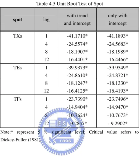
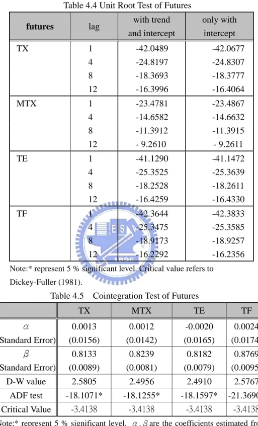
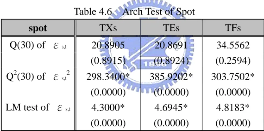
(9) 4.1 Descriptive Statistic .......................................................................................38 4.2 Unit Root and Cointegration Test ..................................................................41 4.3 Arch Effect .....................................................................................................44 4.4 Out-of-Sample Analysis.................................................................................45 4.4.1 Hedge Ratio ........................................................................................45 4.4.2 Hedging Effectiveness ........................................................................48 Chapter 5 Conclusive Remarks.................................................................................51 5.1 Conclusions....................................................................................................51 5.2 Suggestions ....................................................................................................52 References....................................................................................................................53 Curriculum Vitae..........................................................................................................55. ix.

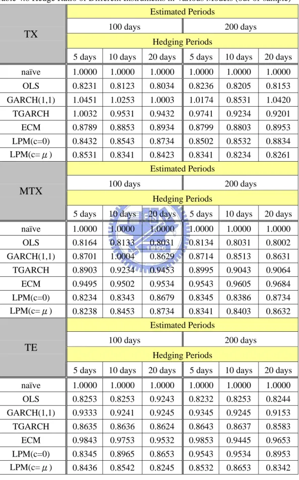
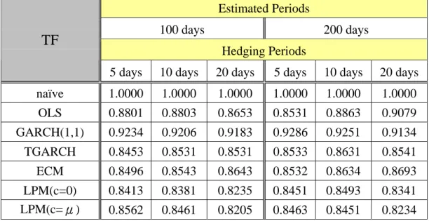
(10) List of Tables Table 1.1 Hedger and Speculator……………………………….………….………….6 Table 4.1 Statistic Descriptions of TXs, TX, MTX…………………………….…….40 Table 4.2 Statistic Descriptions of TEs, TE, TFs,TF………………………………....40 Table 4.3 Unit Root Test of Spot……………………………………………………..42 Table 4.4 Unit Root Test of Futures………………………………………………….42 Table 4.5 Cointegration Test of Futures…………………………………………..….43 Table 4.6 Arch Test of Spot……………………………………………………….….44 Table 4.7 Arch Test of Futures……………………………………………………….44 Table 4.8 Hedge Ratio of Different Instruments in Various Models……….……..….47 Table 4.9 Hedge Effectiveness of HEa in Various Models………………………..….49. x.

(11) List of Figures. Figure 1.1 Research Flow Chart……………………………………………..………...3 Figure 4.1 Scatter Plot of Closing Price in TXs, TX, MTX………………………….39 Figure 4.2 Scatter Plot of Closing Price in TEs, TE………………………………….39 Figure 4.3 Scatter Plot of Closing Price in TFs, TF………………………………….40 Figure 4.4 Dynamic Hedging Process………………………………………………..45. xi.

(12) Chapter 1. Introduction. 1.1 Background and Motivation Since the introduction of Taiwan stock index futures markets in 1997, investors can hedge risk by buying the future contracts. This makes our investment full of variety. Because a stock index futures contract links to the underlying index, it can reflect the price fluctuation in the market. The more the investment channels, the higher degree of risk people are forced to face. Thus, at present, the transaction trust is still weak and the investment risk remains high. This situation may cause the under-performing management, which harms shareholders and the companies. The fund being managed may become risky, for examples, recent scandals happened on Enron, WorldCom and other large companies, whose managers deceived in a manner that eventually bankrupted the companies and destroyed shareholders’ wealth. These events would have influences on people’s desire to enter the investment markets and be harmful to business credit. In this concern, risk management and diminution will become a critical issue. Although all kinds of strategies of the optimal hedge ratio have been addressed in relevant literature, these previous researches only take TAIMEX to practice and do not use the five future contracts of Taiwan for comparison at the same time. For this reason, this article aims to add the other futures index in Taiwan and adopt two major hedging strategies. The first strategy will focus on minimum variances of portfolio. This thesis adopts the naïve, OLS, BI-GARCH(1,1), TGARCH, and ECM model as its representatives. The second strategy is to minimize the downside risk. It can be measured by LPM model.. 1.

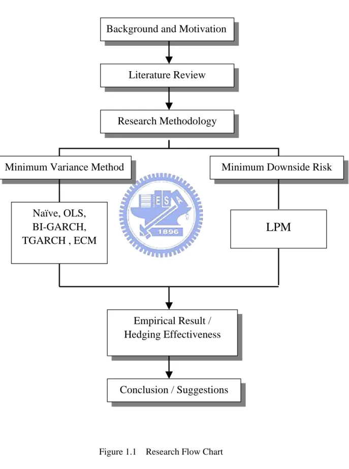
(13) 1.2 Purposes of Study According to what have been mentioned above, the objectives of this study are as follows: (1) To compare the hedging effectiveness between the minimum risk strategy and minimum downside risk strategy. (2) To investigate the implication of different dynamic hedging models. (3) Estimate the hedging effectiveness and optimal hedging ratio of futures with the naive, OLS, bivariate generalized autoregressive conditional heteroskedasticity. (BI-GARCH),. Threshold. generalized. autoregressive. conditional heteroskedasticity (TGARCH), error correction model (ECM), and Lower partial moment (LPM) framework. (4) Discuss the differences of the traditional naïve hedging model with the dynamics model. (5) Investigate the results of hedging effectiveness while the hedging period is expended.. 1.3 Composition of Study This thesis is structured as follows: Chapter 1 describes the motivation, goal, objectives, periods and research structure. Chapter 2 reviews the relevant literature on stock indexes futures, hedging theories and relevant hedging models. Chapter 3 describes the research methodology, including data collection, sampling, and instrument. Chapter 4 illustrates the empirical experiment procedures and examines the relationships of the index futures. Chapter 5 presents the hedging results and empirical finding. Chapter 6 concludes the article and states the limitation, suggestions and economic implications.. 2.

(14) The structure of this research is shown as follows:. Background and Motivation. Literature Review. Research Methodology. Minimum Variance Method. Minimum Downside Risk. Naïve, OLS, BI-GARCH, TGARCH , ECM. LPM. Empirical Result / Hedging Effectiveness. Conclusion / Suggestions. Figure 1.1. Research Flow Chart. 3.

(15) Chapter 2 Literature Review 2.1 Stock Index Futures The stock index is an indicator used to measure and report value changes in a selected group of stocks. It is important that a stock index can track the market movements depending on its composition and the weighing of individual stocks. Besides, the futures contract is a type of derivative instrument, in which two parties agree to transact a set of financial instruments or physical commodities for future delivery at a particular price. In every futures contract, everything is specified: the quantity and quality of the commodity, the specific price per unit, and the date and method of delivery. And the “price” of a futures contract is represented by the agreeable price of the underlying commodity or financial instrument that will be delivered in the future. Therefore, a stock index futures contract has combined the function of two above and made the market more diversified. Trading in futures originated in Japan during the 18th century and was primarily used for the trading of rice and silk. It wasn't until the 1850s that the U.S. started using futures markets to buy and sell commodities such as cotton, corn and wheat. The first index future was born in the Kansas City Board of Trade (KCBT). This contract takes the lead with a future on the Value Line Index, which started trading in February 1982. It took the KCBT five years to get the contract approved. As happens so often in the real world, the first was not always necessarily the most successful. It was the next index launched to become the leader: the S&P 500. The S&P 500 index was introduced in the Chicago Mercantile Exchange (CME) on 21 April 1982. After that, there were more and more other different index futures produced successively. From the viewpoints of Taiwan, the Chicago Mercantile Exchange and Singapore International Monetary Exchange (SIMEX) introduced the first future contract, which treat TAIFEX stock index as underlying asset on January 1997. 4.

(16) This was an important milestone for Taiwan’s future market. Some new financial instruments, including warrant contracts on approved stocks, exchange rate futures and foreign exchange options, were also listed on the Taiwan Stock Exchange or allowed trading over-the-counter in 1997. Following the passage of the Taiwan Futures Trading Law, the local futures exchange was opened in October 1997 and the Taiwan stock index futures (TX) was inaugurated in July 1998. Trading on indexes of electronic sector (TE) and financial sector (TF) futures was open in 1998 to make firms and individuals more flexible in hedging their risks against the volatility of commodity prices, exchange rates, interest rates and stock prices. Subsequently, the mini Taiwan stock index futures (MTX) was launched on April 2001 and provided a smaller contract for investor to transaction. Until now, stock index futures contracts still play an important role in the financial markets. The reason why it can succeed is that index future can reflect fairly the demand and supply of the changeable economic society. There are some vital economic functions of the stock index futures as following. Price Discovery -- Due to its highly competitive nature, the index futures contracts has become an important economic tool to determine prices, based on the estimated demands of today and tomorrow. Futures market prices depend on a continuous flow of information from around the world and thus require a high amount of transparency. Some continuous and open outcry auction is an excellent method for accurately determining the price level, while the information constantly changes the price of a commodity. This process is known as price discovery. Risk Reduction -- Futures markets are also a place for people to reduce risk when making purchases. Risks are reduced because the price is pre-set, therefore letting participants know how much they will need to buy or sell. This helps reduce the ultimate cost to the retail buyer, because with less risk there is less chance of manufacturers jacking up prices to make up for losses in the cash 5.

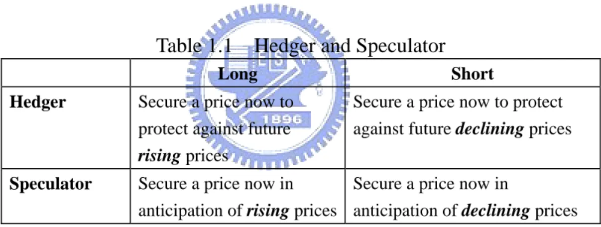
(17) market. Speculation -- Speculation involves the buying, holding, and selling of stocks, commodities, futures, currencies, real estate, or any valuable thing to profit from price fluctuations as contrary to buying it. The players in the futures market fall into two categories: hedgers and speculators. A hedger buys or sells in the futures market to secure the future price of a commodity intended to be sold at a later date in the cash market. This helps protect against price risks. However, a speculator aim to benefit from the every price change, while a hedger focus on protecting themselves against. Speculators want to increase their risk and therefore maximize their profits and hedgers want to minimize their risk no matter what they're investing in. Table 1 illustrates the major distinction between hedger and speculator.. Table 1.1 Hedger and Speculator Long. Short. Hedger. Secure a price now to protect against future rising prices. Secure a price now to protect against future declining prices. Speculator. Secure a price now in Secure a price now in anticipation of rising prices anticipation of declining prices. Arbitrage -- The investor can simultaneous purchase and selling of an asset to profit in different price. This usually takes place on different exchanges or marketplaces. Also known as a "riskless profit". In the process of risk arbitrage, traders can find opportunity to profit and make the price of spot and future close to each other. Therefore, the existences of future markets contribute to improving the efficiency of the financial markets. Diversification Investment -- Owing to the underlying object of stock index future is stock index, the calculation has regulator formulation and not. 6.

(18) easy to be manipulated. Besides, investors spend less money buying the whole stock market commodities indeed make the investment channel greatly diversified. The unique aspects of futures markets, as compared with other marketplaces, have been the focus of discussion. For the most part, hedging techniques involve using complicated financial instruments known as derivatives, the two most common of which are options and futures. This dissertation takes hedging function of futures as a starting point. From the viewpoints of investors with spot market position usually take an opposite contract position in the futures market, being used as a hedge strategy to reduce risks.. 7.

(19) 2.2 Review of Hedging Theory Hedging is a multivariate process for managing risks and achieving objectives. The process of hedging is not the simple buying or selling of futures and options against physicals. It is the prudent selection process whereby regulatory, financial, operational, supply and demand, and other factors must be continually evaluated in order to derive the maximum benefits from the process. There are a broad variety of hedging theories available, which provide a decision rule for people to hold the futures contracts and spot commodity. First of all, Gray and Rutledge (1971) categorized hedge theory into four groups by means of the purpose of hedging, including risk elimination, risk reduction, profit maximization, and portfolio approach. Ederington (1979) showed that the future hedging theories could be classified as three groups: traditional hedging theory, selective hedging theory, and portfolio hedging theory. The traditional hedging theory was inconsistent with reality situation and selective hedging theory not only concerned hedging strategy but also involved in speculative strategy. In general, most of financial assumption took minimizing risks as investors’ hedging strategy. Therefore, the portfolio hedging theory was the most common method to be used nowadays. Among those, Junkus and Lee (1985) adopted profit maximization, risk elimination, risk minimization and utility maximization as the hedging strategy in an empirical study. Cecchetti, Cumby and Figlewski (1988) used risk minimization and maximized expected utility theory to estimate the optimal futures hedge strategy with spot and futures prices dynamic distribution. The remainder of this section describes the three measures of hedging theories from Ederington’s viewpoints.. 8.

(20) 2.2.1 Traditional Hedging Theory Traditional hedging theory focuses on the ability to reduce risk by using futures contracts. If people are long in the cash market, they take a short position in the futures market and vice versa, because they counteract price changes in the two markets against one another. This traditional view suggests that hedging is carried out to reduce price risk (Cootner, 1967). The equal and opposite hedge strategy assume implicitly that the hedger is unskilled or uninterested in forming expectations on the movements of spot price, and that he derives his profits solely from subjecting the transformation of another commodity (Ward and Schimat, 1979). Thus, this hedger has been viewed as a sort of insurance (Samuelson, 1973) against price risk, and the evaluation of its effectiveness is related to risk elimination. In other words, the traditional approach is to hold equal and opposite positions in the futures market whenever a cash position is held. The positions are supposed to be equal in size and adverse direction. Since it is presumed that cash and futures prices of identical products will nearly be perfectly correlated, losses on one position will be compensated for other position profits. As a result, the traditional approach expects that hedging will virtually eliminate price risk during the investment process. Unfortunately, not all risks are eliminated by traditional hedging method. Under the traditional theory, only the basis risk is zero and can be getting rid of the price risk of the spot position. Therefore, this theory deviated from the truly circumstances in reality.. 9.

(21) 2.2.2 Selective Hedging Theory Holbrook Working (1953) modified the traditional view of hedgers by arguing that the essence of hedging is speculation on the basis. He argued that expected profit maximization, rather than pure risk minimization, is the objective of hedgers. Working’s Hypothesis took a different perspective of futures hedging. He challenged the view that hedgers are pure risk-minimizers. Instead, he believed that hedgers behave much like speculators who decide to hedge or not to hedge according to their expectation of the change in spot-future price relation. Therefore, in the 1960s Holbrook Working categorized alternative motives for the futures hedging and these viewpoints continue to be valid in the 1990s. The three categories are arbitrage hedging, operational hedging, and anticipatory hedging. Arbitrage hedging means that people use the inconsistent of securities value to trade, obtain the risk-free premium through the basis change that has already been anticipated. Operational hedging facilitates commercial business by allowing firms to buy and sell on the futures markets as temporary substitutes for subsequent cash market transactions. Anticipatory hedging involves buying or selling futures contracts by commercial firms in “anticipation” of forthcoming cash market transactions. Price expectations play an important role in this hedge. The selective hedging theory made it clears the speculative aspect of hedging: Price changes will not be offset perfectly in any cash and futures combination. The hedger is trading the risk of holding a commodity unhedged for the smaller risk of changes in the basis (Cootner, 1967). In Working’s model, this speculative aspect of hedging is taken limited, and the positions in the futures and cash markets are determined simultaneously in order to capture increased return arising from relative fluctuation in spot and futures prices. 10.

(22) Working used an examination of the year-to-year constancy of the relation between the size of the “spot premium” (means basis) and the gain or loss from subsequent storage with hedging in wheat. At last, the theory detected that a large negative basis (cash price subtract futures price) was likely to be followed by a large positive change in the basis, and that a large positive basis was followed by a large negative change in the basis.. 2.2.3 Portfolio Hedging Theory The traditional hedging theory emphasized on risk reduction, while the selective hedging theory considered making the expected utility maximization. The approaches above were partial and cannot be represented the reality financial markets. However, the portfolio hedging theories integrate these concepts and believe that both reduce the risk and maximize the expected utility should be considered together while hedging. This kind of hedging behavior will also be accordant with common people's behavior. A portfolio explanation of hedging was first strictly presented and developed by Telser (1958), Stein (1961), and Jahnson (1960), who used the Markowits (1959) conceptions of portfolio management. With this approach a hedger is viewed as being able to hold several different cash and futures assets in a portfolio and is assumed to maximize the expected value of his utility function by choosing among the alternative portfolios on the basis of their means and variances. Serveral researchers have drawn on this framework such as Johnson and Steim (1960), Anderson and Danthine (1981), and Howard and D'Antonio (1984). The early researches about portfolio hedging theory can be taken as "minimum variance hedge approach". Johnson (1960) and Steim (1961) applied the Markowitz two-product portfolio model to spot and futures markets. Their approach has been widely used because it provides a method to identify the 11.

(23) minimum-variance portfolio for each level of return. In this model, the hedger is essentially infinitely risk-averse, and defines risk in terms of the variance of his total position in the spot and futures markets. The variance of the return on a hedged portfolio is minimized and the hedge ratio is expressed in terms of expectations on the variation of price changes in the spot and futures markets. Johnson's model differs from Working's in that the objective is to minimize risk and that the position is defined in terms of absolute rather than relative price changes. Anderson and Danthine (1981) proposed the maximized expected utility hedging model. A mean-variance utility formulation is used to obtain operational results to generate the optimal hedge ratio. The framework is equivalent to expected-utility maximization where net revenues are distributed normally and agents' utility functions are exponential. Under the maximization utility model, the theory obtained the following conclusion. First of all, the optima positions of spot and futures are determined simultaneously and the existence of hedge opportunities will influence decision. Secondly, a perfect hedge strategy can be reached by using the multiple-contracts portfolios. Thirdly, a hedger's strategy is depended on the correlation of expected spot and futures price. At last, the optimal hedging strategy concerns not only the minimized risk but also maximized expected utility for the portfolio hedging. Howard and D'Antonio (1984) considered that previous researches did not submit. appropriate. risk-return. measurement. criterions. about. hedging. effectiveness. However, Howard and D'Antonio proposed that hedging effectiveness was seen as comprising both risk and return components. The major foundation of this theory is to utilize the mean-variance analysis to maximize excess return of per unit risk. This theory indicated that hedging effectiveness does not always improve as the spot-future correlation coefficient increases, but depends heavily on the risk-return relative. It was found that this practice can be decomposed into two components: one solely determined by the 12.

(24) futures market conditions, the other affected by both cash and futures markets as well as the hedger's cash portfolio. As the result, the model illustrates that when the risk-return relation is equal to the spot-future correlation coefficient, there is no benefit to holding futures.. 2.3 Lower Partial Moment Theory Portfolio theory is the application of decision-making tools in risk to manage the risky investment portfolios. There have been numerous techniques developed over the years in order to implement the theory of portfolio selection. However, another strategy can be applied is downside risk measurement. The most commonly used of downside risk methods are the semivariance and the lower partial moment (LPM). In addition, the semivariance has been used in academic research in portfolio theory as long as the variance. Markowitz (1952) provided a preliminary framework for measuring the portfolio downside risk by using the semivariance. He employed the means of returns, variances and covariances to derive an efficient frontier where every portfolio on the frontier maximizes the expected return for a given variance or minimizes the variance for a given expected return. Then Bawa (1975) and Fishburn (1977) developed the research on downside risk with the lower partial moment. Bawa was the first to define LPM as a general family of below-target risk measures, one of which was the below-target semivariance. He has argued that LPM model, which based on downside risk measures, is more general than the traditional minimum-variance strategy. This model requires some restrictions on utility functions or the return distribution. For any distributions, it requires the evaluation of the LPM functional for all possible target rates of returns. Bawa (1975) provided a proof that the LPM measure is mathematically. 13.

(25) related to stochastic dominance for risk tolerance values, denoted as n, of 0, 1, and 2. The LPMn=0 is sometimes called the below target probability. The later in Fishburn’s (1977) work insisted that this risk measure is appropriate only for a risk-loving investor. LPMn=1 has the unmanageable name of the average downside magnitude of failure to meet the target return (expected loss). Again, the name of this measure is misleading because LPMn=1 assumes an investor who is neutral towards risk and, in actuality, is a very aggressive investor. LPMn=2 is the semivariance measure, which is sometimes called the below target risk measure. This name is more appropriate to portfolio selection than the other measures, since it actually measures below target risk and is consistent with a risk-averse investor. There is no limitation to what value of n should be used in the LPM except that we have to make a final calculation, i.e., the only limitation is our computational machinery. The n value of risk tolerance degree does not have to be a whole number. It can be fractional or mixed. It is the myriad values of n that make the LPM wide shield. It is also used to describe what an investor considers to be risky. There is a utility function inherent in every statistical measure of risk. We can’t measure risk without assuming a utility function. The variance and semivariance only provide us with one utility function. The LPM provides us with a whole horizon of utility functions. This is the source of the superiority of the LPM risk measure over the variance and semivariance measures. The complete descriptions of the LPM can be obtained in chapter 3.. 14.

(26) 2.4 Relevant Literature Research 2.4.1 Foreign Empirical Results 1.. Junkus and Lee（1985） A study was performed to test the applicability of traditional commodity futures hedging models to the new stock index futures contracts. Four models of hedging behavior applied to stock index futures are examined: (1) A variance-minimizing model introduced by Johnson (1960), (2) The traditional one to one hedge, (3) A utility maximization model developed by Rutledge (1972), and (4) A basis arbitrage model suggested by Working (1953). An optimal ratio or decision rule is estimated for each model, and measures of the effectiveness of each hedge are devised. Each hedge strategy performed best according to its own criterion. The Working decision rule appeared to be easy to use and satisfactory in most cases. Although the maturity of the futures contract used affected the size of the optimal hedge ratio, there was no consistent maturity effect on performance. Use of a particular ratio depends on how closely the assumptions underlying the model used to generate it approach a hedger's real situation.. 2. Ghosh（1993） A paper extends the traditional price change hedge ratio estimation method by applying the theory of cointegration to hedging with stock index futures contracts for S&P 500 index, Dow Jones Industrial Average (DJIA) and NYSE composite index. The sample is daily data and the period is from January 1990 to December 1991. The finding of this study indicated that the hedge ratios obtained from the error correction method are superior to those obtained from the traditional method as evidenced by the likelihood ratio test and out-of-sample forecasts. The improved optimal hedge ratios appear to reduce 15.

(27) considerably the risk of minimizing portfolio. Finally, out-of-sample forcasts from ECM perform better than traditional methods.. 3.. Park and Switzer（1995） Under the minimum risk strategy, this study estimates the optimal hedge ratio in the form of return rate. The data consists of daily closing prices for the S&P 500 index and the Toronto 35 index from June 8 1988 to December 18 1991. The hedging performances are compared in-sample and out-sample with the models of naïve, OLS, OLS with cointegration (OLS-CI) and bivariate GARCH model between spot and futures. Maximum likelihood estimation is used to estimate the parameters in each of the models. The vital results can be concluded as followed. First, the hedging effectiveness of bivariate GARCH model is better than other model. Second, bivariate GARCH model still outperform after considering the transaction cost. At last, the performance of GARCH model gives a superior expression no mater S&P 500 index or Toronto 35 index.. 4.. Holme（1996） Hedging effectiveness is examined for the FTSE-100 Stock Index futures contract from 1984 to 1992. The appropriate econometric technique to use in estimating minimum variance hedge ratios is investigated by undertaking estimations using OLS, and ECM and GARCH. Simple OLS outperforms more complex econometric techniques. Additionally, the impact of hedge duration and time to expiration on estimated hedge ratios and hedge ratio stability over time is examined. It is shown that hedge ratios and hedging effectiveness increase with hedge duration, hedge ratios have duration effects and while hedge ratios vary over time they are stationary.. 16.

(28) 5.. Eftekhari（1998） This article adopts LPM method to estimate the optimal hedge ratio with dynamic rolling technique. The underlying asset is FTSE-100 index from 1985 to 1994. The conclusions can be summarized as three points: (1) If the investor concerns overall risk, minimum-risk strategy is the best strategy. If the investor concerns downside risk, LPM strategy is the best strategy. (2) The hedge ratio in LPM usually smaller than minimum-risk strategy in research. (3) The hedge ratio in LPM can provide a better combination of return and premium.. 6.. Lien and Tse（1998） This article examines the performance of various hedge ratios estimated from different econometric models. The LPM strategy with Asymmetric Power ARCH model (APARCH) is introduced as a new model for estimating the hedge ratio. The object is Nikkei 225 from January 1989 to August 1996. The analysis identifies that the hedge ratio is larger than it is in minimum risk strategy except the target return is –1.5%. While the risk tolerant is bigger and the target rate of return is smaller, the difference of hedge ratio between LPM and minimum risk strategy will become widen. Finally, as the target rate of return is bigger than –1%, the volatility of hedge ratio is no difference between LPM and minimum risk strategy. As the target rate of return is less than –1%, the volatility of hedge ratio in LPM is bigger than minimum risk strategy.. 7.. Yeh and Gannon（2000） The constant and dynamic hedge models, with the presence of transaction costs are compared for the share price index futures contract trading on the Sydney Futures Exchange. The optimal hedge ratio is estimated by conditional hedge ratios. Daily data on spot and futures market is from 1988 to 1996. The portfolio constructed under the GARCH model makes the most profit, while the 17.

(29) naïve model makes the least. The out-of-sample forecasted performance in GARCH model appears to capture arbitrage opportunities. Besides, when portfolio projections are compared base on their profit positions (net of transaction costs), the GARCH hedge model dominates the next best competitor in terms of trading profit.. 8.. H.N.E. Bystrom (2003) This article looks at electricity futures and how they can be used for short-term hedging. The traditional naive hedge and the OLS hedge are compared out-of-sample to more elaborate moving average and GARCH hedges. By using the minimum variance hedge ratio to evaluate the effectiveness, the daily spot and futures prices from Nord Pool, 2 January 1996 to 21 October 1999 obtains the following results. People can make gains from hedging with futures despite the lake of straight-forward arbitrage possibilities. Furthermore, this study indicates that the simple OLS hedge has a slightly better performance to the conditional hedges.. 2.4.2 Domestic Empirical Results 1. Cheng-Hung Wang (1999) This paper extends the traditional price change hedge ratio estimation by applying the model of NAÏVE, OLS, ECM, GARCH, Q-GARCH, and TFARMA to examines the hedging effectiveness of TAIMEX index futures with different intervals. All are daily data, and the sample period is from 21 July 1998 to 31 March 1999. The major results are summarized as follows. First of all, hedge ratio is less than one and the longer of hedge time makes the hedge ratio decline. Besides, the hedge performance and risk reduction in ECM model is outperformed.. 18.

(30) 2. Chih-Liang Wei (2001) This paper estimates the risk-minimizing futures hedge ratios for four types of stock index futures: S&P 500 index futures, Nikkei 225 index futures, MSCI Taiwan index futures and CAC 40 index futures. It compares the hedging effectiveness of traditional model with time-varying model. OLS model, error correction model, univariate GARCH, bivariate GARCH model and Kalman filter are involved. The main empirical results are as follows: 1. There are a significant evidence of unit roots and the relationship between spot and futures prices have cointegration effect. 2. In terms of the within-sample hedging effectiveness comparison, the bivariate GARCH model outperforms all other hedging models except S&P500 stock index. 3. In the out-of-sample comparison, the results are not consistent. The univariate GARCH model outperforms all other hedging models in S&P 500. In Nikkei 225, the Kalman filter is superior to all other hedging models; In MSCI Taiwan index, the ECM model is the best; In CAC 40, the OLS model outperforms all other hedging models.. 3. Michael Huang (2002) The research uses two hedging strategies including minimum variance (MV) approach and minimum downside risk approach. To compare the hedging effectiveness, there are several models about OLS, Near-VAR, ECM, LPM and VaR to be considered. And sample period extends from July 1998 to September 2001. The major results are summarized as follows: 1. No matter what futures or index to employ, hedging strategies will perform better generally when the estimation period or hedging period increased. 2. If the hedger cares the effectiveness of variance deduction, he should adopt Near-VAR-GARCH model with TX or VECM-GARCH model with MTX. 3. If the hedger cares the effectiveness of utility increasing degree, they should use ECM model whatever the futures is.. 19.

(31) 4. Yu-Jiuan Hung (2002) This article has investigated the dynamic relationship between return and volatility in the Taiwan stock index and stock index futures. The bivariate EGARCH error correction model is used in this study. The empirical results show that, there is a strong inter-market dependence not only in the returns of the cash and futures market, but also in the volatility of the two markets. The volatility in both markets is highly persistent and is found to be an asymmetric function of past innovation. Results indicate that the short run dis-equilibrium (measured by error correction term) is responsible not only for returns but also for volatility (measured by conditional variance) of the two markets. These results imply that more precise specification of return and volatility in the two markets may be obtained by including the above factors found in these two markets.. 5. Wei-Chu Lin (2003) Several approaches with different hedge ratios, such as OLS, single GARCH, BI-GARCH, TRI-GARCH, and TRI-EGARCH, are applied. To estimate the effectiveness the data period from July 1998 to March 2003 are collected and transferred to returns of single-day, 5-day, 10-day, and 20-day for the comparison of the effectiveness with different approaches. The conclusion is that local futures market has a better correlation with local spot market and a better performance on a specific stock than overseas futures market does. Therefore an investor owning local spot should pursue better hedging effectiveness by adopting local futures rather than oversea ones. Hence an investor should adopt proper approach portfolio by considering different hedging periods to pursue best hedging effectiveness.. 6. Yi-Ling Chen（2004） The study investigates the price discovery and lead-lag relationships in the 20.

(32) three markets: "Taiwan stock index-Taiwan stock index futures", "Taiwan stock index-Taiwan Top 50 Tracker Fund", and "Taiwan stock index futures-Taiwan Top 50 Tracker Fund". The main research is to examine all data with error-correction models, Granger causality test and EGARCH model. Results of the study show that Taiwan stock index futures lead spot and Taiwan Top 50 Tracker Fund.. 21.

(33) Chapter 3. Research Methodology. 3.1 Data Source This study investigated the out-of-sample hedging effectiveness from 10th April 2001 to 30th April 2006 daily 1,256 observations. The underlying assets include Taiwan weighted stock index (TXs), electronic sector index (TEs), financial sector index (TFs), Taiwan stock index futures (TX), mini Taiwan stock index futures (MTX), electronic sector index futures (TE), and financial sector index futures (TF). If there were no transactions in some day, the data would be deleted. The prices quoted in Taiwan Economics Journal databank (TEJ) 1,256 observations are obtained. The calculating tools we adopt are Eviews 5.0 and Matlab 6.0. This paper confines the analysis to the near contract because preliminary research showed that there is not very much difference between the hedging properties of the nearest and the second contract. The trading volume of nearby contract is greater, and the nearby contract can be representative of the long-term relationship of spot and futures. Owing that there are five future contracts of different months in the markets everyday, this study adopts the nearby contract as the best choice. The definition of nearby contract here is –The data on five days before last trading day is quoted price on that month, while the data from next day to the last day of month is regarded at next month quotation. This study takes the daily stock index with the associated stock index futures to compute its daily rate of return. The rate of returns is computed by differentiating the logarithm of the daily stock index and futures index. Besides, the hedging periods of this article are setting at one day, one week (5 days), and one month (20 days). The rate of return on spot and futures are computed as follows:. 22.

(34) The stock index spot rate of return is calculated as:. R xs , t = ( ln Px , t s − ln Px , t − 1 s ) × 1 0 0. (3.1). Where Rxs,t = the daily return of the spot x at time t, ln Px ,t s = the closing prices of the stock index for spot x at time t, ln Px ,t −1s = the closing prices of the stock index for spot x at time t-1.. The stock index futures rate of return is calculated as: R xf, t = ( ln Px , t f − ln Px , t − 1 f ) × 1 0 0. (3.2). Where Rxf,t ：= the daily return of the futures x at time t, ln Px ,t f = the closing prices of the stock index for futures x at time t, ln Px ,t −1 f = the closing prices of the stock index for futures x at time t-1.. 23.

(35) 3.2 Unit Root Test and Cointegration Test When we begin to form models for time series, we have to check whether the underlying stochastic process that generated the series is invariant with respect to time. If the trends of the stochastic processes are fixed in time, one can model the stationary process through an equation with fixed coefficients that can be estimated from past data. Although the traditional OLS approach often assumes the time series are stationary and its disturbances are almost white noise. Granger and Newbold (1974) have proposed that if we assume the non-stationary time series as stationary to analysis, it may result in "spurious regression" situation. It will cause the problem that a higher coefficient of determination (R2) and a lower Durbin-Watson value (a much significant t value). Therefore, we should check whether the properties of all variables are stationary before analysis. If the time series become stationary through the process of k-times differentiate, it can be significantly reject the alternative hypothesis and is called integrated of order n as I(k). That means the series I(1) has one unit root. There are plenty of methods to measure the stationary test. The most famous test is the Dickey-Fuller test, the Phillips-Perron test, and the Augmented Dickey-Fuller (ADF) unit root test. This study follows the method of the Augmented Dickey-Fuller unit root test.. 3.2.1 Augmented Dickey-Fuller Test According to the AR (1) process proposed by Dickey and Fuller (1979), a simple AR(1) model is: Yt = α 0 + α1Yt −1 + ε t. (3.3). where the εt is white noise error term. This model can be estimated and tested for a unit root with the null hypothesis ofα1=1. If it is rejected, the series is 24.

(36) stationary statistically. This is so-call DF (Dickey-Fuller) test. The above-mentioned DF test must assume the error term is white noise. While it always happen that the residual term of regression equations reveal autoregressive situation. The range of test may be restricted by the DF test. If the series is correlated at higher order lags, the assumption of white noise disturbance is violated. Therefore, Dickey and Fuller (1981) made a parametric correction for higher-order correlation by adding the lags term of the dependent variable in the left side and adjusting the test methodology. The main purpose of this process is to eliminate the series correlation. Following shows the general form of the process. p. Yt = α1Yt −1 + ∑ βiYt −i + ε t. Pure Random Walk. (3.4). Yt = α 0 + α1Yt −1 + ∑ β iYt −i + ε t. Random Walk with Intercept. (3.5). i =1. p. i =1. p. Yt = α 0 + α1Yt −1 + β T + ∑ β iYt −i + ε t. Random Walk with Intercept. i =1. and Time Trend. (3.6). Unless we know the actual data-generating process, it is a problem to concern whether it is most appropriate to estimate (3.4), (3.5), (3.6). It is important to use a regressed equation that mimics the actual data-generating process. This specification is used to test H0: α1=0. If the result rejects null hypothesis, it means the time series are stationary without unit root vice versa.. 3.2.2 Cointegration Test After examining the variable stationary property, we examine whether there is any cointegrating relationship, to appropriately construct the following other models. Engle and Granger (1987) recognized that a linear combination of two or more non-stationary series might exist stationarity. If such a stationary, or I(0), linear combination exists, the non-stationary time series are said to be cointegrated. This can be interpreted as a long-term equilibrium relationship between variables. 25.

(37) According to Engle and Granger's statements, a stochastic process with no deterministic components is defined to be integrated of order d, denoted I(d). Let vector Xt subjects to I(d), if there exists a vector α(≠0) such that Zt=α'Xt ~ I(d-b), b>0, the components of the vector Xt are said to be cointegrated of order (d, b). Usually the case with d=b=1 is considered. The general estimated method is the two-stage analysis which testing the cointegration between variables by estimating the serial correlation of residuals estimated from OLS approach mainly. Another method of cointegration test is Johansen's (1988) procedure which maximizing the canonical correlation between the first differenced series and the level series. This method followed the idea of Engle and Granger and proposed the maximum likelihood ratio test. The great contributions of it are extended the analysis structure from two variables to more variables and employ the trace and maximal eigenvalue statistic to estimate the numbers of cointegrating vector. The main assumptions of both tests is that series are exactly I(1).. Yt = α + β X t + ε t. Yt and Xt ~ I(0). (3.7). This study investigated the Johansen's (1988) approach to make the cointegrate test. We firstly use OLS method to estimate the long-term relation of spot and futures index returns as equation (3.7), called cointegrating regression. Secondly, test and verify the residual term does not have unit root so that cointegrating relationship exists. Further, The Akaike Information Criteria (AIC) and the Schwarz criteria (SC) can be used to choose the optimal lag length. This article adopted the minimum AIC criteria to determine the lag terms.. 26.

(38) 3.3 Residual Test 3.3.1 Autocorrelation Residual Test The Durbin-Watson (1950) is used to test the presence of first-order autocorrelation in the residuals of a regression equation. The test compares the residual in time t with the residual in time t-1 and develops a statistic that measures the significance of the correlation between these successive comparisons. The formula for the statistic is: n. ∑ (e − e DW =. t =2. t −1. t. )2 (3.8). n. ∑e t =1. 2 t. et = Yt − Ylt. (3.9). The statistic can be used to test the presentation of both positive and negative correlation in the residuals. The critical value of upper limit (dU) and lower limit (dL) can be taken by checking the professional table. The following is the decision criteria.. positive correlation 0. cannot judgment dL. no correlation dU. 4-dU. cannot judgment. negative correlation 4-dL. 4. If the data appears a higher-order autocorrelation, the Durbin-Watson test cannot be used. Ljung and Box (1978) proposed the following (3.10) Q statistic to measure the circumstances. The Ljung-Box Q statistic is corresponding to the kth autocorrelation test whether the first k autocorrelations are zero, as white noise. Under the null hypothesis of no autocorrelation the Q statistic is distributed chi-square with q degrees. Where ρk is the k-th autocorrelation and. 27.

(39) T is the number of observations.. ρ k2. q. Q = T (T + 2)∑ k =1. (3.10). (T − k ). 3.3.2 ARCH Effect Test The previous research has found that many of the time series data follow the three features: leptokurtic, fat tails, and volatility clustering. These situations can. be. precisely. be. observed. by. the. Autoregressive. Conditional. Heteroskedasticity (ARCH) model. Besides, the generation of the General Autoregressive Conditional Heteroskedasticity (GARCH) model is to correct the residual heteroskedasticity of the Ordinary Lest Square (OLS) model. Because that when the error term has heteroskedastic variance, the OLS no longer satisfy BLUE presupposition. Therefore, we have to make the ARCH test for residual terms before estimating the hedge ratio with GARCH model. The general method of testing is Lagrange Multiplier Test, briefly named ARCH-LM test. The process is as following. The autoregressive model is. ε t = yt − xt a ,. (3.11). ε t = vtσ t2 ,. (3.12). and vt ~ N (0,1). The variance equation can be displayed as (3.12) while the ARCH (q) exists. If there were no ARCH effect, the variance is a constant. It 2 means σt =α0. The null assumption is H0: α1=α2=…=αq. σ t2 = α 0 + α1ε t2−1 + α 2ε t2− 2 + ... + α qε t2− q. (3.13). One then estimates the equation (3.12) and computes the R-square. Come after the test statistic and its asymptotic distribution are given by ARCHLM(q) = T*R2 ~ χ2(q) and T is the total amounts of samples.. 28. (3.14).

(40) 3.4 Hedging Strategy and Model 3.4.1 Hedging Strategy This paper employs the two strategies to analysis the hedging effectiveness of the four kinds of stock index futures in Taiwan. The first is focus on minimum variances of portfolio hedging strategy. This thesis uses the naïve, OLS, BI-GARCH (1,1), TGARCH, and ECM model as representative. The second strategy is to make the downside risk minimum. It can be measured by LPM model. By using the fundamental hedging model to estimate its hedge ratios in these two strategies, and the detail descriptions is introduced as bellow. Individual stocks and all stock portfolios, except for those specifically designed to have zero beta, are exposed to some market risk. The purpose of first strategy is to make the variance minimum. This article adopts the minimum variance model of Johnson (1960) and Ederington (1979) as analysis foundation. Assuming that the only hedging instrument available to the investor is the futures contract, a hedge portfolio consisting of spot and futures is constructed. Let St+1 and ft+1 is the changes in spot and futures price, respectively, between time t and t+1, and ht is the hedge ratio at time t. Then the return to a trader going long in the spot market and going short in the futures market with ht units at time t is Xt+1:. Xt+1＝St+1－ht ft+1. (3.15). vart ( X t +1 ) = vart ( St +1 ) + ht2 vart ( f t +1 ) − 2ht covt ( St +1 , ft +1 ). (3.16). The variance of this return portfolio is displayed in equation (3.15) and the minimum variance ratio, ht*, can be derived by simply minimizing this variance with respect to ht. The symbols of σs andσf mean the variances of spot and futures, and σsf is covariance between spot and future. To find the constant hedge ratio that minimizes risk, we differentiate (3.15) once with respect to vart(Xt+1) equal to zero and ends up with the following expression for ht*: 29.

(41) ht * =. covt ( St +1 , ft +1 ) σ sf = 2 vart ( f t +! ) σf. (3.17). The second strategy of this article is to make the downside risk minimum. It can be measured by Lower Partial Moment (LPM) model. The first person used the semivariance to measure the loss risk is Markowitz (1959). He recognized d that investors are interested in minimizing downside risk for the two reasons that only downside risk is relevant to an investor and the security distributions may not be normally distributed. Therefore a downside risk measure would help investors make proper decisions when faced with unnormal security return distributions. Markowitz shows that when distributions are normally distributed, both the downside risk measure and the variance provide the correct answer. 2. 1 k SVm = ∑ max[0, ( E − RT )] k T =1 SVt =. 1 k [0, (t − RT )]2 ∑ k T =1. (3.18). (3.19). However, if the distributions are not normally distributed only the downside risk measure provides the correct answer. There were two kinds of methods to measure the downside risk from Markowitz: a semivariance computed from the mean return or below-mean semivariance (SVm) and a semivariance computed from a target return or below-target semivariance (SVt). These two measures compute a variance using only the returns below the mean return (SVm) or below a target return (SVt). Since only a subset of the return distribution is used, Markowitz called these measures partial or semi- variances. The lower partial moment function is derived from the conceptions of SVt. This theory describes the below-target risk in terms of risk tolerance. Given an investor risk tolerance value n, the general measure of the lower partial moment, is defined as:. 30.

(42) c. LPM (c, n, rp ) = E[max(0, c − rp ) n ] = ∫ (c − rp ) n dF (rp ) , −∞. (3.20). where c is the target return, n is the degree of the lower partial moment, and rp is the return for the portfolio during time period of T. The symbol of F(․) means the distribution of rp and the "max" is a maximization function which chooses the largest of 0 or (c- rp). This thesis computes the LPM by adopting the risk tolerance degrees is 2, which is the opinion of Markowitz (1959) proposed. It is the only considering that the target returns are c=0 and the mean of return on spot during historic periods (c=μ). Therefore, we can obtain the equation (3.21) by substituting (3.14) for (3.20). LPM (c, 2, rp ) = E[max(0, Rth+1 − Rts+1 + bt Rt f+1 )]2 = E[max(0, c − rs + brf )]2. (3.21). While partial differentiate at equation (3.21) with bt, and then the optimal hedge ratio (hlpm) which is under the minimum lower partial moment can be obtained and N is the amount of sample. N. N. ∑rr. hlpm =. rp ≤ c. s f. − c ∑ rf rp ≤ c. N. ∑r. rp ≤ c. (3.22). 2 f. 3.4.2 Naïve Model The naïve model directly adopts the 1:1 hedge ratio to avoid the risk. That is, the traditional hedger's concepts. The theory insists people should hold equal amounts in futures market to hedge the spot position. This is so-call that classic hedge ratio claims for a futures position that is equal but opposite in sign to the cast position.. 31.

(43) 3.4.3 OLS Model The use of ordinary least square (OLS) model to evaluate the hedge ratio is the most convenient way and the calculation is easier than other methods. Benninga et al. (1984) derived the minimum-variance hedge ratio from an ordinary least squares (OLS) regression with cash price levels (or price changes) as the dependent variable and futures price levels (or price changes) as the explanatory variable. The minimum-variance hedge ratio is simply the slope coefficient of the OLS regression, or equivalently: h* =. cov( spot , futures ) var( futures). (3.23). This ratio was developed as the optimal hedge ratio for any unbiased futures market.. If the futures market is unbiased, the only advantage to. hedging is to reduce risks associated with deviations from the expected income. By using the minimum-variance hedge ratio, a producer will eliminate the maximum amount of uncertainty that can possibly be eliminated by hedging. Therefore, if the futures market is unbiased, the minimum-variance hedge ratio will always be the optimal hedge ratio for any risk averse producer regardless of the degree of risk aversion. Thus, each minimum-variance hedge ratio will be determined by the slope coefficient and the hedging effectiveness will be measured by the R2 coefficient from an OLS regression of cash price changes on futures price changes.. 3.4.4 GARCH Model It has long been recognized that heteroskedasticity can pose problems in ordinary least squares analysis. The standard warning is that in the presence of heteroskedasticity, the regression coefficients for an ordinary least squares regression are still unbiased, but the standard errors and confidence intervals estimated by conventional procedures will be too narrow, giving a false sense of 32.

(44) precision. The ARCH and GARCH model can solve the problem of the conditional variance.The most widely used specification is the GARCH (1,1) model introduced by Bollerslev (1986) as a generalization of Engle(1982). The (1,1) in parentheses is a standard notation in which the first number refers to how many autoregressive lags appear in the equation, while the second number refers to how many lags are included in the moving average component of a variable. The GARCH (1,1) model can be generalized to a GARCH (p,q) model; that is, a model with additional lag terms.. Such higher order models are often. useful when a long span of data is used, like several decades of daily data or a year of hourly data. With additional lags, such models allow both fast and slow decay of information. A particular specification of the GARCH (2,2) by Engle and Lee (1999), sometimes called the component model, is a useful starting point to this approach. Thus, a GARCH (p,q) model for hedging strategy looks like this: St = a + hf t + ε t. (3.24). ε t | Ωt −1 ~ N (0, σ t2 ). (3.25). σ t2 = α 0 + α1ε t2−1 + δ1σ t2−1. (3.26). Where St = return rate of spot, ft = return rate of futures, a = intercept. h = optimal hedge ratio.. Park and Switzer (1995) proposed that the hedge ratio should be a dynamic form when the distributions of spot and futures price vary with time path. The bivariate distributions of spot and futures are as follows.. 33.

(45) st = a0 + a1 ( St −1 − γ Ft −1 ) + ε st. (3.27). ft = b0 + b1 ( St −1 − γ Ft −1 ) + ε ft. (3.28). ⎡ ε st ⎤ ⎢ ⎥ | Ωt −1 ~ N (0, H t ) ⎣⎢ ε ft ⎦⎥ ⎛ hss ,t Ht = ⎜ ⎝ hsf ,t. where. (3.29). hsf ,t ⎞ ⎛ hs ,t ⎟=⎜ h ff ,t ⎠ ⎝ 0. 0 ⎞⎛ 1 ⎟ h f ,t ⎠ ⎜⎝ ρ. ρ ⎞ ⎛ hs ,t ⎟⎜ 1 ⎠⎝ 0. 0 ⎞ ⎟ h f ,t ⎠. (3.30). hst2 = cs + α sε s2,t −1 + β s hs2,t −1. (3.31). h 2ft = c f + α f ε 2f ,t −1 + β f h 2f ,t −1 ,. (3.32). St = return rate of spot, ft = return rate of futures, εst = residual term of spot, εft = residual term of futures, Ωt-1 = information set of time t-1,. Ht = covariance metric of time t, ρ= coefficient of correlation betweenεst andεft .. In this paper we adopt above approach and use the maximum likelihood estimate (MLE) to acquire the hedge ratio, h* . h* =. h sf ,t. (3.33). h f ,t. Another version of GARCH models takes an asymmetric view by estimating positive and negative returns separately. Typically, higher volatilities follow negative returns than positive returns of the same magnitude. The threshold ARCH (TGARCH) model is one of asymmetric approach to compute. The descriptions are as following.. 34.

(46) (1) Conditional Mean Equation ⎛ St ⎞ ⎛ B11 ⎞ ⎛ B12 ⎜ ⎟ = ⎜ ⎟+⎜ ⎝ Ft ⎠ ⎝ C11 ⎠ ⎝ C12. B13 ⎞ ⎛ St −1 ⎞ ⎛ ε w,t ⎞ ⎟ ⎟×⎜ ⎟+⎜ C13 ⎠ ⎝ Ft −1 ⎠ ⎝ ε s ,t ⎠. ε t | Ωt −1 ~ N (0, ht ). (3.34) (3.35). (2) Conditional Variance Equation ⎛ hs ,t ⎞ ⎛ VC11 ⎞ ⎛ VA11 VD11 ⎞ ⎛ hs ,t −1 ⎞ ⎛ VB11 VE11 ⎞ ⎛ ε s2,t −1 ⎞ ⎜ ⎟=⎜ ⎟+⎜ ⎟+⎜ ⎟×⎜ h ⎟ × ⎜⎜ 2 ⎟⎟ h VC VA VD VB VE − , , 1 f t f t 22 22 22 22 22 ⎝ ⎠ ⎝ ⎠ ⎝ ⎠ ⎝ ε f ,t −1 ⎠ ⎝ ⎠ ⎝ ⎠. (3.36). ⎛ hsf ,t −1 ⎡⎣ hsf ,t ⎤⎦ = [VC12 ] + [VA12 ] × ⎜ ⎝ 0. (3.37). 0 ⎞ ⎟ h fs ,t −1 ⎠. Where St = return rate of spot, Ft = return rate of futures, Ωt-1 = information set of time t-1,. hs,t = conditional variance of spot return at time t, hf,t = conditional variance of futures return at time t, hsf,t = conditional variance of spot and futures time t. B12 = the effect of St-1 on St ,. B13 = the effect of Ft-1 on St,. C12 = the effect of St-1 on Ft ,. C13 = the effect of Ft-1 on Ft,. B. and B11,C11,VC11,VC22,VC12 are all intercepts, VA11 = the effect of volatility of St-1 on volatility of St, VD22 = the effect of volatility of Ft-1 on volatility of Ft, VD11 = the effect of volatility of St-1 on volatility of Ft, VA22 = the effect of volatility of Ft-1 on volatility of St, VB11 = the effect of shock of St-1 on volatility of St, VE22 = the effect of shock of Ft-1 on volatility of Ft 35.

(47) VE11 = the effect of shock of St-1 on volatility of Ft, VB22 = the effect of shock of Ft-1 on volatility of St, VA12 = the covariance of St-1 and Ft-1 . According to the maximum likelihood estimator (MLE) method, we can obtain the following hedge ratio: h* =. hsf ,t. (3.38). h f ,t. 3.4.5 ECM Model Engle and Granger (1987) suggested that we should avoid losing long-term information by using the cointegration method to illustrate the long-term relationship between variables and resolve the doubts of losing information due to the differential process. They showed that as long as two economic variables are cointegrated (even if the variables are affected by certain factors in the short-term and turn into a process of random walks), they would return to the long-term equilibrium through the process of the dynamic short-term adjustment. From the viewpoints of Granger, cointegrate is corresponding with error correction model (ECM). If the cointegrated effect exists, the error correction model can be constructed as following: m. n. i =1 m. nj =1. i =1. j =1. +S t = α 0 + α1μt −1 + b+ f t + ∑ d i + f t −i + ∑ θ j +St − j + ε t. (3.39). + f t = β 0 + β1μt −1 + c+St + ∑ ei +St −i + ∑ θ j + ft − j + ut. (3.40). where △St represents the rate of return for spot market, △ft is the rate of return for futures market, μt-1 is the error correction term, εt and ut shows the stationary errors at time t, and the hedge ratio is b. It can be observed that the ECM model adds the error correction term, which was from the cointegrating regression, into autoregressive model. That is, the ECM model considers not only the long-run equilibrium but also the short-run (error correction term) adjustment processes. 36.

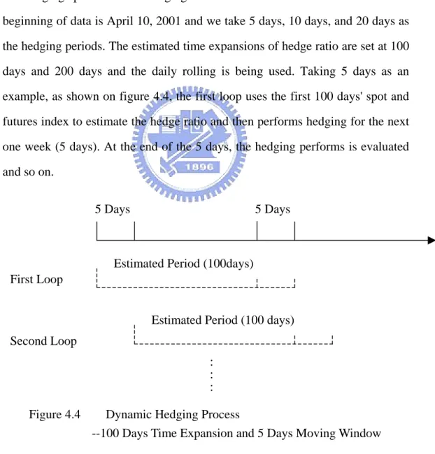
(48) 3.5 Hedging Effectiveness The variance's reduction of the predicted returns in an unhedged spot portion can be used to evaluate hedging performance. That is, the greater the risk reduces, the better the hedging performance will be. The first hedging effectiveness is derived from Ederington's (1979) conception. Assuming that the hedger has one unit spot position (price is St-1) at time t-1, he decides to short at time t with St. Then the unhedged return and variance is shown in equation (3.41) and (3.42): E(U)＝E(△St). (3.41). Var(U)＝Var(△St),. (3.42). where △St= St－St-1 .If the hedger wants to hedge and sell the future position with b unit, the portfolio expected return and variance after hedging is as bellow: E(H)＝E(△St)－b E(△Ft). (3.43). Var(H)＝Var(△St)－2bCov(△St , △Ft)＋b2Var(△Ft). (3.44). where △Ft= Ft－Ft-1. The effectiveness of the minimum-variance hedge can be evaluated by examining the percentage of risk reduced by the hedge (Ederington, 1979). Hence, the measure of hedging effectiveness is also defined as the ratio of the variance of the unhedged position minus the variance of the hedged position, over the variance of the unhedged position: HEEderington =. Var (U ) − Var ( H ) Var (U ). (3.45). In order to compute the average hedging effectiveness, the method of moving window has been adopted. The overall hedging effectiveness can be evaluated by the equation (3.46), HEa, where n is the times of rolling. The higher the number is, the better the dynamic hedging performance is. n. HEa =. ∑ HE i =1. (i ) Ederington. (3.46). n 37.

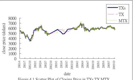
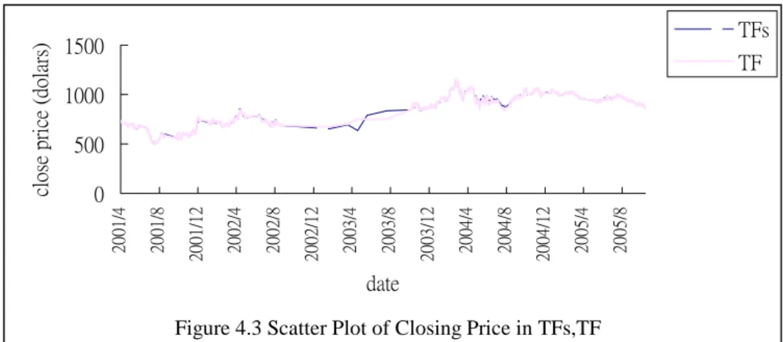
(49) Chapter 4 Empirical Analysis 4.1 Descriptive Statistic The implementation of this paper methodology is now summarized as follows. First, choose a underlying sample. Second, pre-written the unhedged portfolio and futures returns. There is some evidence that daily stock index returns display significant and persistent autocorrelation in both levels and in volatility. Hence, it has been down to calculate the return and analysis the data descriptions. Once it is satisfied with stationary process, then proceed in third stage by estimating the optimal hedge ratio of each different model. In the forth stage this paper move x days forward, the updating and rebalancing frequency, and compute the out-of-sample hedging error from t+1 to t+x. Then it is necessary to return to stage 2 and reiterate the procedure until the results arrive at the most recent observation. In stage fifth, this paper try to compute the variance of the accumulated series of hedging errors and express this as the hedged risk reduction, and obtain the hedging performance by equation (3.46). Finally, compare the hedging performances of the competing models. The scatter plots of daily closing price between spot and futures shows in figure (4.1) to figure (4.3). It is displayed that four kinds of underlying index near to homogeneous. This paper uses TXs, TEs and TFs as the symbol for TAIFEX stock index, electronic sector stock index and financial sector stock index. Besides, the symbols of MTX, TX, TE and TF represent as mini Taiwan stock index futures, Taiwan weighted stock index futures, electronic sector index futures and financial sector index futures, respectively. It can be observed that the trends of futures price corresponding to the trends of spot price. This shows the highly correlation between each other. The preliminary descriptions of data from July 10, 2001 to October 21, 2005 are showed in table (4.1). But only the MTX have lower mean and different standard deviation. This is because the MTX has different contract 38.