利用模糊類神經網路之音頻信號分類與切割技術

全文

(1)國立交通大學電機與控制工程學系碩士論文. 利用模糊類神經網路之音頻信號分類與切割技術 Audio Classification and Segmentation Technique Using Fuzzy Neural Networks. 研究生：陳瑞正指導教授：林進燈. 博士. 中華民國九十四年七月.

(2) 利用模糊類神經網路之音頻信號分類與切割技術 Audio Classification and Segmentation Technique Using Fuzzy Neural Networks. 研究生：陳瑞正. Student：Jui-Cheng Chen. 指導教授：林進燈博士. Advisor：Dr. Chin-Teng Lin. 國立交通大學電機與控制工程學系碩士論文. A Thesis Submitted to Department of Electrical and Control Engineering College of Engineering and Computer Science National Chiao Tung University in Partial Fulfillment of the Requirements for the Degree of Master in Electrical and Control Engineering July 2005 Hsinchu, Taiwan, Republic of China. 中華民國九十四年七月. i.

(3) 利用模糊類神經網路之音頻信號分類與切割技術. 學生：陳瑞正. 指導教授：林進燈博士. 國立交通大學電機與控制工程研究所摘. 要. 在本論文中我們提出了一個針對音頻信號之分類與切割的系統，此系統可將含有靜音、純語音、純音樂以及歌曲之檔案，根據其類型加以分類與切割。我們針對上述各種音訊的特徵的作分析與比較，並根據這些分析與比較的結果，設計一套分類流程將輸入的音訊分兩階段依序完成分類與切割。一開始的靜音偵測根據一個門檻值標示出音訊中屬於靜音的部分。之後，第一階段將輸入音訊中非靜音部分分為純語音與「含有音樂成分」兩類，第二階段將在第一階段中被歸類為「含有音樂成分」的部分，進一步分為純音樂以及歌曲。為了解決傳統特徵在進行純音樂與歌曲分類時分類效果不佳的問題，本論文提出了一個名為「前三峰值之頻率變化量(FVTP)」的新特徵。此特徵描述了歌曲的頻譜結構會隨著時間而顯著地改變而純音樂之頻譜結構改變量相對較小之特性。因此該特徵能在進行純音樂與歌曲分類時，改善分類效果不佳的問題。而在分類器的選用方面，本系統採用一前向式自我建構類神經模糊推理網路(SONFIN)做為核心分類器。該網路具有可自我建構並調整的架構與參數學習的功能，以及優異的模糊類神經推論過程。我們利用這些特性達到較佳之分類結果。實驗結果顯示，本系統可達到平均 90%以上的分類正確率。因此，本系統可作為許多如語音辨識、語者辨識等應用系統的前端處理，使輸入這些應用系統的內容符合系統要求以提升應用系統的效能。. i.

(4) Audio Classification and Segmentation Technique Using Fuzzy Neural Networks Student: Jui-Cheng Chen. Advisor:. Dr. Chin-Teng Lin. Institute of Electrical and Control Engineering National Chiao-Tung University. ABSTRACT In this thesis, we proposed an audio classification and segmentation system. The system is used to classify and segment audio files which contain silence, pure speech, pure music, and song according to their contents. We analyzed and compared features of audio signals and designed a two-stage classification flow to classify and segment input audio signals sequentially. The flow starts with the silence detection which indexes silence according to a threshold. Then, stage 1 classifies the nonsilence parts into pure speech and “with music components”. Stage 2 classifies the “with music components” parts in stage 1 into pure music and song. In order to solve the problem that traditional features do not work well when it comes to pure music/song classification, we proposed a novel feature named FVTP. The feature describes the property that variations of the spectrum structure are larger for song but smaller for pure music. Thus, the feature can improve the performance of pure music/song classification. On the other hand, an on-line self-constructing neural fuzzy inference network (SONFIN) was adopted as the main classifier in this system. The SONFIN finds its optimal structure as well as parameters automatically and it has a superior inference process. We achieved a better classification result by utilizing these properties. Experimental results showed that an accuracy rate of more than 90% was achieved. Thus, the proposed system is capable of being a front-end for many application systems such as speech recognition and speaker identification to improve the performance of these application systems.. ii.

(5) 誌. 謝. 本論文能順利完成實需感謝眾多師長同學的指導與幫助。首先感謝指導教授林進燈博士這兩年來的指導與提攜，在研究上一方面給予我極大的自由度，讓我能完全的發揮想像力與創造力，而另一方面研究在遇到瓶頸時，亦提供了我正確的方向，使研究能繼續順利進行。其次要感謝的是實驗室的劉得正學長，學長在研究的細節上給了我許多的幫助與建議，讓我在能很快的瞭解這個研究領域。此外也要謝謝實驗室裡眾多的學長、同學與學弟們，在日常生活中的協助與陪伴，讓研究的日子充實也充滿歡笑。最後感謝家人的支持，讓我沒有後顧之憂地完成我的學業。. iii.

(6) Contents Chinese Abstract.................................................................................... i Abstract ................................................................................................. ii Acknowledgement ............................................................................... iii List of Figures ...................................................................................... vi List of Tables ...................................................................................... viii Chapter 1 Introduction .........................................................................1 1.1 1.2 1.3. Motivation....................................................................................................1 The Goal of the Research.............................................................................3 Thesis Organization .....................................................................................5. Chapter 2 Background..........................................................................6 2.1 2.2. Related Works ..............................................................................................6 Introduction to Audio Signal Processing ...................................................10 2.2.1 The Characteristics of Audio Signals................................................10 2.2.2 Audio Signal Processing Techniques................................................12 2.2.2.1 Short Time Analysis of Audio Signals .....................................13. Chapter 3 Audio Feature Analysis and Selection .............................17 3.1 3.2 3.3 3.4 3.5 3.6. Zero-Crossing Rate ....................................................................................19 Spectrum Flux............................................................................................22 Normalized Root Mean Square Variance...................................................24 Low Short-Time Energy Ratio...................................................................27 High Zero-Crossing Rate Ratio .................................................................28 Frequency Variation of Top-3 peaks ..........................................................29. Chapter 4 SONFIN-Based Audio Signal Classification and Segmentation System ..........................................................................38 4.1 4.2. Neural Fuzzy Inference Network...............................................................38 Classification Flow and Post-processing ...................................................41. Chapter 5 Experimental Results ........................................................46 5.1 5.2 5.3. Audio Database..........................................................................................46 Evaluation with SONFIN and k-NN ..........................................................46 Discussion ..................................................................................................51 iv.

(7) Chapter 6 Conclusion..........................................................................53 References.............................................................................................55. v.

(8) List of Figures Fig. 1 The proposed ASC system...................................................................4 Fig. 2 A 10-second audio signal...................................................................13 Fig. 3 The first 600 points of the signal in Fig. 2.........................................14 Fig. 4 The concept of short-time analysis and a hamming window.............15 Fig. 5 Two major components of pattern classification. ..............................17 Fig. 6 ZCR and variance of ZCR..................................................................20 Fig. 7 ZCR_var histograms for speech and music signals...........................21 Fig. 8 Spectrum flux values. ........................................................................23 Fig. 9 SF histograms for pure speech and the signals with music components. .........................................................................................23 Fig. 10 SF histograms for pure speech and song. ........................................24 Fig. 11 The normalized RMS variance value of a period of speech and signal with music components. ............................................................26 Fig. 12 Normalized RMS variance histograms for pure speech and the signals with music components. ..........................................................26 Fig. 13 LSTER values..................................................................................28 Fig. 14 HZCRR values.................................................................................29 Fig. 15 ZCR_var histograms for pure music and song. ...............................30 Fig. 16 SF histograms for pure music and song...........................................30 Fig. 17 Normalized RMS variance histograms for pure music and song. ...31 Fig. 18 Five adjacent frames of pure music.................................................32 Fig. 19 Five adjacent frames of song. ..........................................................33 Fig. 20 Five adjacent frames of speech........................................................34 Fig. 21 (a) A 1-second music waveform with two notes. (b) RMS of 40 frames of the signal in (a) ....................................................................35 Fig. 22 The differences between 40 RMSs ..................................................35 Fig. 23 The transition point is marked by ‘o’. .............................................36 Fig. 24 FVTP histograms for pure music signals and song .........................37 Fig. 25 Network structure of SONFIN. .......................................................39 Fig. 26 The proposed audio classification flow. ..........................................42 Fig. 27 The concept of “smoothing”............................................................44 Fig. 28 Result of practical audio stream classification and segmentation in stage 1. .................................................................................................50 Fig. 29 Result of practical audio stream classification and segmentation in stage 2. .................................................................................................50 vi.

(9) Fig. 30 practical experimental result of music and song. ............................51. vii.

(10) List of Tables TABLE I Relation between physical and perceptual features. .................... 11 TABLE II Classification performance of different features in stage 1 ........47 TABLE III Classification performance of different features in stage 2.......48 TABLE IV Classification performance of stage 2 with the influence of stage 1............................................................................................................48 TABLE V Classification performance of speech/song discrimination ........49. viii.

(11) Chapter 1 Introduction 1.1 Motivation Sound is an extremely useful medium for conveying information. In addition to explicit semantic information such as the meaning of words used in speech, the acoustic signals conveyed to our ears carry a wealth of other information. These signals play important roles in our daily life. For example, audio including music, speech and kinds of sound is indispensable in modern multimedia applications which become essential in human’s daily life with the development of digital technology such as computers and digital signal processing. With these digital technologies, audio signals can be sampled, digitized, processed and stored in digital form. Furthermore, in order to benefit from digital signals, it is important to dig out different contents of audio by some signal processing methods according to different applications. One of these applications is classifying audio signals automatically which is interesting for people since humans classify audio signals all the time. To tell the difference between music and speech, to recognize which word is pronounced, and to identify one speaker to another are named speech/music classification, speech recognition and speaker identification, respectively [1], [2]. All of these tasks can be viewed as audio signal classification (ASC) problems. As mentioned in the previous paragraph, speech/music classification 1.

(12) is one of ASC domains. More precisely speaking, speech/music classification is a front-end for other ASC domains. The front-end processing is important because different types of audio need different processing techniques. Only with a good speech/music classifier can we have a better input for speech recognition systems or musical genre classifiers. For example, a speech recognition system assumes input is speech, and a musical genre classifier can work well only when input is music. Another example is that a system designed to translate broadcast news into text on radio channels will work better if the unknown input stream (which may consist of music and speech) is segmented and classified first. On the other hand, since the amount of audio data in multimedia databases and on the Internet increases swiftly, to retrieve the data manually becomes more and more impossible. Furthermore, most search engines nowadays like Google and Yahoo are text-based. Therefore, it seems to be a “mission impossible” for one who is not good at memorizing names to search databases and the Internet for audio data. Thus, ASC systems which can segment, classify, index, and retrieve audio data automatically according to its contents are now necessary. Take a realistic application for example, after indexing an audio database with the ASC technique, a song can be retrieved by humming the tune of it. This is a useful system since people sometimes can only remember the melody of a song instead of its title.. 2.

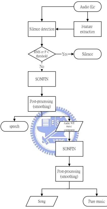
(13) 1.2 The Goal of the Research In the thesis, we developed an audio classification and segmentation system and focused on the differences between instrument music, speech, song and silence. This is an important and challenging topic since neither in time domain nor in frequency domain are these signals readily separable. However, these classes of signals are common in our daily life. In order to classify these signals with high accuracy for practical applications, it is essential and indispensable to analysis the signals. We applied some signal processing techniques on the signals to acquire some good features, which are critical to get great accuracy. Then, we analyzed the features and compared their properties. In the thesis, features such as zero-crossing rate, spectrum flux, and normalized RMS variance and so on are applied since their distributions are different for different types of audio signals. After grasping the distributions of these features in different types of audio signals, we can integrate the features and set a classification flow which is based on the concept of decision trees and applies an on-line self-constructing neural fuzzy inference network (SONFIN) to classify the signals with different content sequentially with a high accuracy rate. Figure 1 shows the ASC system proposed in the thesis. Audio features are first extracted. Then, silence segments are detected and indexed according to some features extracted in the previous step. The non-silent sounds are classified into speech segments and segments with music components. After that, segments with music components are categorized into two groups, namely song and pure music. We will 3.

(14) discuss the processes in detail in the latter chapters.. Fig. 1 The proposed ASC system.. 4.

(15) 1.3 Thesis Organization The thesis is organized as follows. In chapter 2, related works will be reviewed and some audio signal processing techniques will be briefly introduced for further discussion. In chapter 3, we give a detail analysis of features used in our system. Chapter 4 discusses the proposed audio classification system which includes a neural fuzzy inference network, and the post processing process. The experimental results are shown in chapter 5, and some comments are also provided. Chapter 6, which summarizes the thesis, will give concluding remarks and possible future works.. 5.

(16) Chapter 2 Background 2.1 Related Works As mentioned previously, ASC includes many research areas such as speech recognition, music genre classification, speaker identification, and so on. Although research in speech recognition, a domain of ASC, has existed for many years [3], there were not significant research output in other areas of ASC until recent years (after 1990’s). Some of related works on this topic will be presented in the following paragraphs. In [4], audio was classified into music, speech and others. For music, the system computes peaks in the magnitude spectrum, and then bases its decision on the average length of time that peaks exist in a narrow frequency region. To separate out speech, the pitch track is examined. Kimber and Wilcox [5] classified and segmented discussion recordings in meetings into speech, silence, laughter, and nonspeech sound using cepstral coefficients and a hidden Markov model (HMM). In [6], Pfeiffer et al. presented the analysis of the amplitude, frequency, pitch, onset, offset and frequency transitions of audio signals. With the analysis results, violence in movie soundtracks can be detected by recognizing shots, cries and explosions. Furthermore, music indexing can be an application of the analysis results. In [7], the goal of automatic retrieval, classification and clustering of musical instruments, sound effects, and environmental sounds can be 6.

(17) achieved by using statistical values (mean, variance, autocorrelation) of features (pitch, loudness, brightness, and bandwidth). In the article, some applications such as audio databases and file systems, audio database browsers, audio editors, and surveillance were also provided. A simple approach to discriminate music from speech was presented by John Saunders [8]. The discriminator used straightforward features such as the energy contour and the zero-crossing rate (ZCR). Experiments were performed with four measures of the skewness of the distribution of ZCR, and 90% correct classification rate was obtained using these features. Improved performance of 98% correct classification rate was reported by including an energy contour dip measure into the discrimination process. Scheirer and Slaney [9] introduced 13 features for speech/music discrimination. Statistical pattern recognition classifiers such as MAP, GMM, and KNN were evaluated. They used a 2.4-second window and got an error rate of 1.4%. When smaller windows as well as more classes were taken into consideration, the error rate would increase. A method for content-based audio classification and retrieval was presented in [10]. The audio feature vector, named PercCepsL, consisted of an 18-dimensional perceptual feature vector and a 2L-dimensional cepstral feature vector. The perceptual feature vector was composed of the silence ratio, the pitched ratio, the means and standard deviations of total power, 4 subband powers, brightness, bandwidth and pitch. The 2L-dimensional cepstral feature vector came from the L MFCCs. A new pattern classification method called the nearest feature line (NFL) was also reported in this paper. Applying the proposed method to the audio 7.

(18) database of 409 sounds from Muscle Fish, NFL+PercCeps8 yielded the lowest error rate of 9.78%. Zhang and Kuo [11] proposed a heuristic rule-based ASC system. The system was divided into two stages. They used four features including the energy function, the average zero-crossing rate, the fundamental frequency, and the spectral peak tracks to achieve classification accuracy of more than 90%. Lu et al. [12] classified an audio stream into speech, music, environment sound and silence using a robust two-stage audio classification and segmentation method. The features which were selected for classification such as high zero-crossing rate ratio (HZCRR), low short-time energy ratio (LSTER), spectrum flux (SF), band periodicity (BP), noise frame ratio (NFR), and LSP distance measure were described and discussed. An accuracy rate of over 96% was reported. In [13], an audio clip was classified into five classes—silence, music, background sound, pure speech, and nonpure speech by using kernel SVM with Gaussian Radial basis. The feature set included 8 order MFCCs, zero-crossing rates (ZCR), short time energy (STE), sub-band powers distribution, brightness, bandwidth, spectrum flux (SF), band periodicity (BP), and noise frame ratio (NFR). The accuracy rate of the proposed method using SVM distributed from 87.62% to 96.20% for each individual class. Panagiotakis and Tziritas [14] dealt with the characterization of an audio signal and developed a system for speech/music discrimination. They fitted the amplitude distribution measured by the root mean square. 8.

(19) (RMS) with the generalized χ 2 distribution, and used the distribution to segment an audio signal. And then these segments were classified into music and speech by utilizing five actual features (normalized RMS variance, the probability of null zero-crossings, joint RMS/ZC measure, silence intervals frequency, and maximum mean frequency) deriving from two basic characteristics, i.e. the amplitude and the zero-crossings. The proposed system segmented signals with an accuracy rate of about 97% and classified signals with an accuracy rate of about 95%. Although most of the systems mentioned previously classify general audio signals into various classes such as speech, pure music, song etc, some systems specifically aimed to classify musical genres [15]–[17]. In [18], Tzanetakis and Cook proposed three feature sets which resulted in a 30-dimentional feature vector to describe timbral texture, rhythmic content and pitch content. After feature extraction, they used standard statistical pattern recognition classifiers for classification. Several classifiers such as Gaussian classifiers, Gaussian mixture model (GMM) classifiers, and K-nearest neighbor (KNN) classifiers were trained to evaluate the proposed feature sets, and an accuracy rate of 61% for 10 genres was achieved by using GMM classifiers. To deserve to be mentioned, although the above systems mainly focus on processing audio signals individually, it is intriguing that audio segmentation and classification can be applied to video indexing. Researches showed that audio parts are often more useful than the visual images for indexing films or news programs [19]. In [20], an audio-based approach for video indexing was provided. Minami et al. applied image 9.

(20) processing techniques to analyze the spectrogram of audio signals in video, and detect music by image edge detection. After detecting music components, the music components were removed from speech detection. Speech detection was then accomplished by a comb filter. After music and speech detection, they used the information to construct two video indexing systems. In this thesis, we focus on audio classification and segmentation, a critical problem in audio content analysis. Some audio signal processing techniques utilized in the thesis are provided in the following section.. 2.2 Introduction to Audio Signal Processing An audio signal is an extremely useful medium for conveying information. Humans are surrounded by audio signals as long as he or she is able to listen. In this section, we will introduce some important characteristics of audio signals related to audio signal classification, and audio signal processing techniques in order to extract information from these characteristics.. 2.2.1 The Characteristics of Audio Signals An audio signal, i.e. sound, is a form of energy. After vibrating, an object will carry particles of the air near the object and produce a longitudinal wave with velocity about 343 meters per second. The frequency of a wave refers to how often the particles of the air vibrate when a wave passes through the medium. The frequency of a wave is 10.

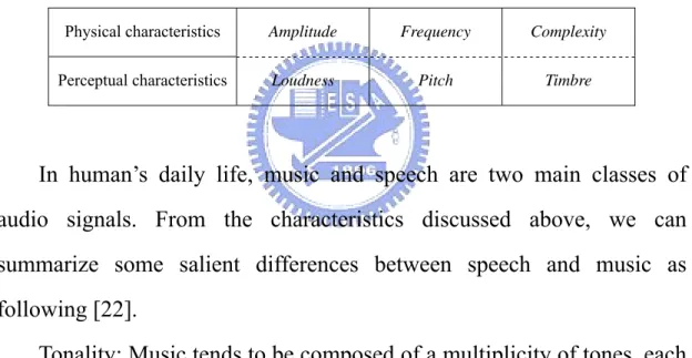
(21) measured as the number of complete back-and-forth vibrations of a particle of the medium per unit time. In addition to frequency, sound has two other important characteristics, amplitude and complexity. These three physical characteristics influence three perceptual characteristics, pitch, loudness, and timbre, respectively. Roughly speaking, human can perceive what kind of sound he or she hears because the characteristics of each kind of sound are different. TABLE I lists the relationship [21].. TABLE I Relation between physical and perceptual features. Physical characteristics. Amplitude. Frequency. Complexity. Perceptual characteristics. Loudness. Pitch. Timbre. In human’s daily life, music and speech are two main classes of audio signals. From the characteristics discussed above, we can summarize some salient differences between speech and music as following [22]. Tonality: Music tends to be composed of a multiplicity of tones, each with a unique distribution of harmonics. Speech consists of an alternating sequence of tonal and noise-like segments. Bandwidth: The frequency of music is up to 20000 Hz while the frequency of speech is limited to 4000 Hz. Energy sequences: Music usually has more stable energy sequences than speech does. Some of these characteristics might be helpful to discriminate 11.

(22) between these two kinds of audio signals, and they can be extracted using signal processing techniques. As mentioned previously, an audio signal can be represented as a function of density of air varying with time. Thus, it is a continuous function. In order to be processed in a computer, the function needs to be sampled and digitized, and becomes a discrete-time audio signal. There are two parameters, i.e. the sampling rate and the bit resolution which influence the quality of the digital signal. Any discrete-time audio signal can be created by adding infinite number of discrete-time sinusoidal signals with different frequencies and amplitudes. That is s[n] = ∑ Ak cos(ωk n) .. (2.1). k. This implies that we can decompose an audio signal into its component sinusoids. To perform the function, we need Fourier analysis, which will be introduced in the following subsection.. 2.2.2 Audio Signal Processing Techniques With the development of digital technology such as computers and digital signal processing (DSP), not only audio signals can be sampled, digitized, processed and stored in digital form, but also complex algorithms are able to be implemented cheaply and speedily. In this section, we will discuss short time analysis of audio signals owing to the non-stationary property of audio signals.. 12.

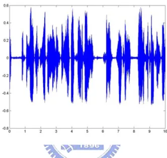
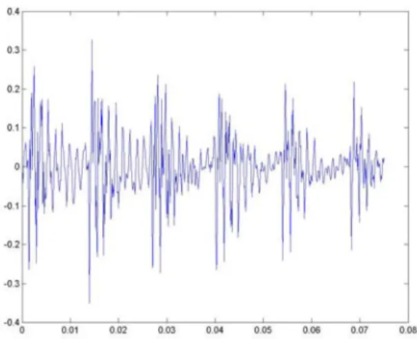
(23) 2.2.2.1 Short Time Analysis of Audio Signals [23] Generally speaking, an audio signal is time-varying. That is, the signal changes rapidly with time. Fig. 2 is an example of a 10-second audio signal. It has a quite large variation and lacks a regular pattern.. Fig. 2 A 10-second audio signal.. As we can see, it is difficult to acquire effective information from this kind of time-varying signal. However, when we examine the signal from a micro standpoint, the signal is stable and has a regular pattern as illustrated on Fig. 3. The waveform is extracted from the first 600 points of the signal in Fig. 2.. 13.

(24) Fig. 3 The first 600 points of the signal in Fig. 2.. Thus, most audio signal processing techniques assume that the variation of an audio signal in a short time is relatively small. Based on this assumption, every small segment of an audio signal is independent of each other, and the properties in a single segment are fixed. Therefore, we can view the small segments as short-time stationary signals. These small segments are called frames. To deal with these frames, short-time processing techniques are adopted. Most of the short-time processing techniques can be represented mathematically in the form. Qn =. ∞. T [ x(m)]w(n − m) ∑ m=−∞. (2.2). The audio signal is subjected to a transform, T[ ], which may be linear or nonlinear. The transform is determined according to what features are to be extracted. Thus, Qn can be viewed as one of features that represent the short-time signal. For example, the short-time energy. 14.

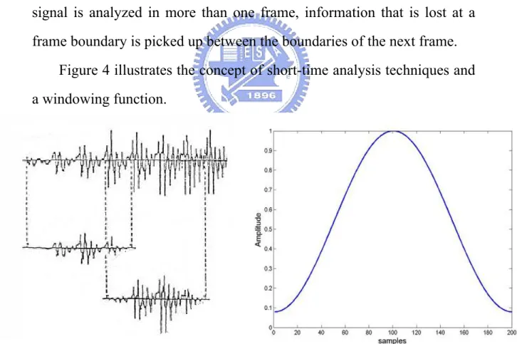
(25) function is defined as En =. 1 [ x(m) w(n − m)]2 . w(n) is a short-time ∑ N m. window such as Gaussian window, Hamming window, and Kaiser window. The function of a window is to gently scale the amplitude of the signal to zero at each end, reducing the discontinuity at frame boundaries. Using no windowing function is the same as using a rectangular window. The windowing functions do not completely remove the frame boundary effects, but they do reduce the effects substantially. When these windowing functions are applied to a signal, it is clear that some information near the frame boundaries is lost. For this reason, a further improvement is to overlap the frames. When each part of the signal is analyzed in more than one frame, information that is lost at a frame boundary is picked up between the boundaries of the next frame. Figure 4 illustrates the concept of short-time analysis techniques and a windowing function.. Fig. 4 The concept of short-time analysis and a hamming window.. 15.

(26) Among various types of short-time signal analysis methods, the Short Time Fourier Transform (STFT) is one of the most common and useful methods, and has the advantage of fast calculation based on the Fast Fourier Transform algorithm. The STFT of the nth frame is define as ⎛ ⎜ ⎝. Xn ⎜e. j 2π k N. ∞ ⎞ − j 2π km N = x ( m ) w ( nL − m ) e ⎟ ⎟ m=−∞ ⎠. ∑. 0 ≤ k ≤ N −1. (2.3). where w(n) is a short-time window, and L is the window length. Many features used in the purposed system are based on the short-time magnitude of the STFT of the signal. The features will be introduced and discussed in detail in the next chapter.. 16.

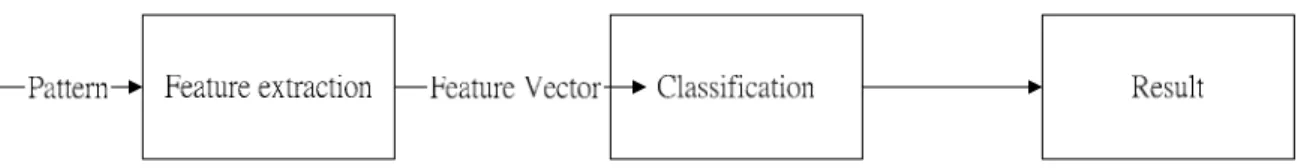
(27) Chapter 3 Audio Feature Analysis and Selection It is difficult to classify audio signals directly based on raw data since raw data contain too much information for analysis, and important characteristics are lost in the noise of unreduced data. Thus, it is necessary to reduce the amount of data. The process is called feature extraction, which computes a numerical representation that can be used to characterize a segment of audio. The important information to characterize a segment of audio is usually in the form of quantities such as frequency, rhythm, pitch and so on. To extraction features or a feature vector (which consists of some features) is the first step in any pattern classification system as shown in Fig. 5. A feature vector can be thought of as a short term description of the sound for that particular moment. For example, MFCCs (Mel-Frequency Cepstral Coefficients) characterize the vocal tract resonances and are commonly used in speech recognition.. Fig. 5 Feature extraction and the classification of the features are two major components of pattern classification.. Typically, the feature vectors are extracted within successive frames that overlap. For example, frames of 20 to 40 milliseconds overlapped by. 17.

(28) 10 milliseconds are often used because characteristics of the signal are relatively stable in this kind of frame. And feature vectors can be extracted from these frames. After representing the raw data with the feature vectors, the audio classification problem can be viewed as a pattern classification problem based on a time series of feature vectors, which are points in a multi-dimensional feature space. In the thesis, we break a long audio signal into small segments and a feature vector is computed for each segment. Therefore, the feature vector can be viewed as points in the feature space. Therefore, our goal is simplified as to classify the points into different classes. Since the goal is to classify the points into different classes, it is true that the more discriminative the features are, the better the problem is solved. However, the problem is how to find a good feature to classify audio signals effectively. As mentioned in the previous chapter, different types of audio signals bear different characteristics. Thus, if we are able to know how the characteristics behave in different types of audio signals, and quantify the characteristics, we can find a good feature for classification. In other words, the knowledge about audio signals is the key point. The features used in audio signal classification systems are usually divided into two categories: perceptual and physical features [24]. Perceptual features rely on a great deal of perceptual modeling. Physical features are directly related to physical properties of the signal and are easier to define and measure. In the following sections, we will introduce main features used in our 18.

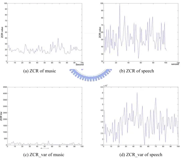
(29) system. All of these features are computed from successive frames of 200 sampling points for a 1-second sample which contains 8000 sampling points. In other words, each frame is 25-millisecond long, and the sampling rate for the audio signals is 8k Hz.. 3.1 Zero-Crossing Rate The zero-crossing rate (ZCR) of the nth frame is defined as ZCRn =. 1 sgn ⎡⎣ x ( m ) ⎤⎦ − sgn ⎡⎣ x ( m −1) ⎤⎦ w ( n − m ) 2∑ m. (3.1). where ⎧1, sgn ⎡⎣ x ( n ) ⎤⎦ = ⎪⎨ ⎪⎩−1,. x ( n ) ≥ 0, x ( n) < 0. x(m) is a discrete time audio signal and w(n) is a 200-sample rectangular window. In other word, ZCR is how often an audio signal goes through the zero point in a frame. The properties of ZCR are different in different types of audio signals. Take speech signals for example, speech signals consist of alternating voiced and unvoiced sounds. For unvoiced sounds, they tend to have higher ZCR. For voiced sounds, they tend to have lower ZCR. Thus, the variation of ZCR of a series of speech tends to be large. On the other hand, music signals usually have lower variation as well as lower ZCR. In this way, we cannot only discriminate unvoiced from voiced speech using ZCR, but also use the variation of ZCR to distinguish between music and speech. The variance of ZCR in a 1-second window is defined as. 19.

(30) (. 1 N ZCR _ var = ∑ ZCRn − ZCR N n=1. ). 2. (3.2). where ZCR is the average of all ZCRs in a 1-second sample. The ZCR and ZCR_var of different type of audio signals in plotted in Fig. 6. As we can see, the ZCR curve of music is relatively smooth, and ZCR_var is smaller. For speech signals, the ZCR curve varies rapidly, and ZCR_var curve is relatively larger.. (a) ZCR of music. (b) ZCR of speech. (c) ZCR_var of music. (d) ZCR_var of speech. Fig. 6 ZCR and variance of ZCR.. Another way to show that ZCR_var can discriminate between speech and music effectively is illustrated in Fig. 7. The figure shows the 20.

(31) histograms of ZCR_var for speech and music signals. The overlap is quite small. If ZCR_var is used alone to discriminate speech from pure music, the discrimination error rate would be only about 9%.. Fig. 7 ZCR_var histograms for speech and music signals.. The most attractive property of ZCR and the variance of ZCR is that these features have slight computation consumption. This is because ZCR can be calculated simply on time domain. Thus, no transformation is needed. This is an important feature for systems which is designed for real-time usage. For example, broadcast monitors which keep monitoring the content of radio to decide whether the content should be discarded is a real-time system. Although ZCR and the variance of ZCR are good features for speech/music discrimination, they are not sufficiently good when it comes to other classification. Thus, other features are necessary for further classification.. 21.

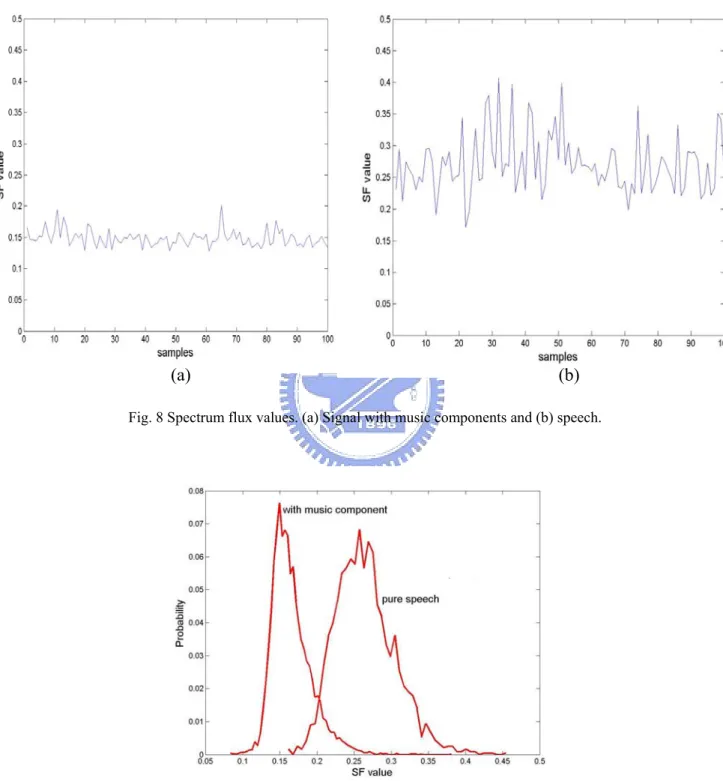
(32) 3.2 Spectrum Flux Spectrum flux measures the average variation value of spectrum. between two adjacent frames in a 1-second segment. It is defined as N −1 K −1 ⎡. ⎤ ⎛ j 2π k ⎞ ⎛ j 2π k ⎞ 1 N N ⎢ SF = log( X n ⎜ e ⎟ + δ ) − log( X n−1 ⎜ e ⎟ + δ )⎥ ⎜ ⎟ ⎜ ⎟ ⎥ ( N −1)(K −1) n=1 k =1 ⎢ ⎝ ⎠ ⎝ ⎠ ⎣ ⎦. ∑∑. ⎛ ⎜ ⎝. where X n ⎜ e. j 2π k N. 2. (3.3). ⎞ ⎟ is the amplitude of the discrete Fourier transform of ⎟ ⎠. the nth frame of the input signal as defined in (2.3) and K is the order of DFT, N is the total number of frames and δ = 0.000001, which is a very small value to avoid calculation overflow. Generally speaking, speech has larger SF value than pure music, song, and mix of speech and music. This is because the tone tends to vary in a short time when human speak, and a music note usually remains at the same level for a certain period of time. When people sing, the vocal sound follows the music note. Thus, the vocal sound also remains at the same level for a certain period of time. The difference between pure music and vocal sound is that vocal sound might lasts for more than one musical note, and vocal cords are apt to vibrate. This causes a ripple-like shape spectrogram and a higher SF value for music. The spectrum flux value of different types of audio signals is plotted in Fig. 8. As we can see, the SF value of speech signals is generally larger than that of signals with music components. From the statistical viewpoint, as shown in Fig. 9, there are small overlaps between the 22.

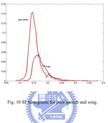
(33) histogram for pure speech signals and that for the signals with music components. Thus, spectrum flux value is another good feature to discriminate speech from signals with music components.. (a). (b). Fig. 8 Spectrum flux values. (a) Signal with music components and (b) speech.. Fig. 9 SF histograms for pure speech and the signals with music components.. Unfortunately, the SF value does not work well if we apply it 23.

(34) independently to discriminate pure music from song. As shown in Fig. 10, their distributions have a significant overlap. Thus, only about 60% average recognition rate can be achieved.. Fig. 10 SF histograms for pure speech and song.. 3.3 Normalized Root Mean Square Variance As we mentioned in 2.2.1, an audio signal is characterized by three physical characteristics, i.e. amplitude, frequency, and complexity. This implies that in addition to information provided by frequency, there should be more information hidden in other characteristics which can help us to classify audio signals. The amplitude, measured by the root mean square (RMS) value, is a good example.. RMS of the nth frame of the input signal is defined as. RMSn =. ⎡ x ( m ) w(n − m) ⎤ ∑ ⎣ ⎦ m. N 24. 2. (3.4).

(35) where w(m) is a rectangular window of length 200-point. Both ZCR and RMS are typical time domain features which can be calculated fast, but they are almost independent [14], [25]. Thus, they are good features to discriminate speech from music simultaneously. As ZCR, the variation of RMS can be applied as a feature since speech tends to have unstable amplitude owing to the pauses between utterances and the voiced and unvoiced components in speech. Although RMS and RMS_var are good features for speech/music discrimination, it fails for some cases that the volume is either extremely large. or. extremely. small.. To. overcome. the. problem,. some. volume-independent feature should be employed. The normalized RMS variance is defined as. σ A2 =. RMS _ Var RMS. (3.5). 2. where. RMS _ Var. variance of RMS in a 1-second window;. RMS. mean of RMS in a 1-second window.. The normalized RMS variance value of a period of speech and signal with music components is plotted in Fig. 11. The plot in Fig. 12 is the histogram for pure speech signals and that for the signals with music components. Both of these two figures reveal that normalized RMS. variance is a good feature to discriminate speech from signals with music components.. 25.

(36) Fig. 11 The normalized RMS variance value of a period of speech and signal with music components.. Fig. 12 Normalized RMS variance histograms for pure speech and the signals with music components.. 26.

(37) 3.4 Low Short-Time Energy Ratio It has been proven that short-time energy is useful in characterizing different audio signals. Furthermore, the variation of short-time energy is more discriminative. A measure of variation of short-time energy called. low short-time energy ratio (LSTER)is defined in [12] as. 1 LSTER = 2N. N −1. ⎡sgn 0.5E − E + 1⎤ ( n) ∑ ⎢ ⎥⎦ n =0 ⎣. (3.6). where En. the short-time energy of the nth frame;. N. the total number of frames;. E. the average of all short-time energy in a 1-second sample;. ⎧1, sgn ⎡⎣ x ( n ) ⎤⎦ = ⎪⎨ ⎪⎩−1,. x ( n ) ≥ 0, x ( n) < 0. The value of LSTER means the ratio of the number of frames whose short-time energy are less than 0.5 time of average short-time energy in a 1-second window. Fig. 13 illustrates LSTER values for a period of speech and music signals. From the distribution, we know that LSTER value of speech is usually larger than that of music. This is because speech signals contain more silence than music signals do. Thus, LSTER is a good feature to classify speech and music signals.. 27.

(38) Fig. 13 LSTER values (0-150 sec is speech, and 151-290 sec is signals with music components).. 3.5 High Zero-Crossing Rate Ratio As mentioned in 3.1, ZCR and its variation are good features to classify speech and music. Thus, a feature called high zero-crossing rate ratio (HZCRR) to quantify the variation of ZCR is proposed in [12]. HZCRR of a 1-second sample is defined as 1 HZCRR = 2N. N −1. ⎡sgn ZCR − 1.5ZCR + 1⎤ ( n ) ⎥⎦ ∑ ⎢ n =0 ⎣. where ZCRn. the zero-crossing rate of the nth frame;. N. the total number of frames;. 28. (3.7).

(39) ZCR. the average of all ZCRs in a 1-second sample;. ⎧1, ⎡ ⎤ sgn ⎣ x ( n ) ⎦ = ⎪⎨ ⎪⎩−1,. x ( n ) ≥ 0, x ( n) < 0. .. The value of HZCRR means the ratio of the number of frames whose ZCR are above 1.5-fold average zero-crossing rate in a 1-second window. Fig. 14 illustrates HZCRR values for a period of speech and music signals. From the distribution, we know that HZCRR is a good feature to classify speech and music signals, too.. Fig. 14 HZCRR values (0-150 sec is speech, and 151-290 sec is signals with music components).. 3.6 Frequency Variation of Top-3 peaks Although the features mentioned in previous sections are excellent features for speech/pure music discrimination, their performance are not sufficiently good when it comes to other kinds of classification such as pure music and song discrimination. Take ZCR_var, spectrum flux, and 29.

(40) normalized RMS variance for examples, their histograms for pure music and song are highly overlapped as shown in Fig. 15, 16, and 17. The solid lines represent histograms for these three features of pure music, and the dot lines represent histograms for these three features of song. Clearly, if only these features are employed for pure music/song discrimination, the recognition rate will take a nosedive.. Fig. 15 ZCR_var histograms for pure music and song.. Fig. 16 SF histograms for pure music and song.. 30.

(41) Fig. 17 Normalized RMS variance histograms for pure music and song.. To sort out the problem, a feature called frequency variation of top-3 peaks (FVTP) was proposed. FVTP was derived from the idea that the spectrum structure of pure music during a note is much more stable than that of song and speech. Fig. 18, 19, and 20 show the spectrums of five adjacent frames of pure music, song and speech, respectively. As we can see, the three largest peaks in the spectrum of music do not change their locations. On the other hand, the locations of the three largest peaks in the spectrum of song vary significantly. Thus, FVTP is defined as the sum of the variations of frequencies of the three largest peaks over 500 Hz in the spectrum during a note (for music) or a word (for song). That is, FVTP of kth note or word is defined mathematically as 3. N. (. FVTPk = ∑∑ f ij − f i i =1 j =1. ). 2. (3.8). where fij is the frequency of the ith peak of the jth frame, f i is the 31.

(42) average frequency of the ith peak in a note or word, and N is the number of frames in a note or word. The average of FVTPs of all notes or words in a 1-second sample is then calculated to be the feature, i.e. FVTP =. 1 K FVTPk . K∑ k =1. (a) The first frame. (b) The second frame. (c) The third frame. (d) The fourth frame. (e) The fifth frame Fig. 18 Five adjacent frames of pure music.. 32.

(43) (a) The first frame. (b) The second frame. (c) The third frame. (d) The fourth frame. (e) The fifth frame Fig. 19 Five adjacent frames of song.. 33.

(44) (a) The first frame. (b) The second frame. (c) The third frame. (d) The fourth frame. (e) The fifth frame Fig. 20 Five adjacent frames of speech.. 34.

(45) To find the boundaries between notes or words in one second, notes or words are segmented by amplitude. First, the average amplitude of the nth frame is calculated by RMSn defined in (3.4). For example, a 1-second music waveform with two notes and its RMSn are illustrated in Fig. 21.. (a). (b). Fig. 21 (a) A 1-second music waveform with two notes. (b) RMS of 40 frames of the signal in (a). Generally speaking, there will be a sudden change in the RMS value when the audio signal changes from one note to another. Thus, in order to locate the point, the differences between RMSs in Fig. 21 should be calculated as illustrated in Fig. 22.. Fig. 22 The differences between 40 RMSs. 35.

(46) Then, all local maximums of RMS differences which are larger than one-fifth of the global maximum of RMS differences are viewed as the transition points as shown in Fig. 23. In this case, only the global maximum of RMS differences is indexed and it is exactly where the note change happens.. Fig. 23 The transition point is marked by ‘o’.. Last of all, two FVTPs are computed separately, and the average of these two FVTPs can be obtained to be the FVTP of the 1-second sample. FVTP is an effective feature to discriminate pure music from song. Generally speaking, vocal components are prominent in song, so peaks in the spectrum are usually generated by vocal components. Vocal components in song might last for more than one musical note and human vocal cords tend to vibrate when singing, so the locations of the top-3 peaks in spectrum will fluctuate constantly. This causes a large FVTP value for song. In contrast, pure music produced by musical instruments normally has a stable spectrum structure and caused a relatively small 36.

(47) FVTP value. Fig. 24 shows the histogram for pure music signals and the histogram for song. As we can see clearly, that FVTP value of pure music is around 0.1×106 , while FVTP value of song is around 0.2 ×106 to 1×106 . Thus, FVTP is a good discriminator between pure music and song.. Fig. 24 FVTP histograms for pure music signals and song. With the features introduced in previous sections, we have accomplished the feature extraction for audio classification. In next chapter, we will step forward to discuss the framework of our audio classification system.. 37.

(48) Chapter 4 SONFIN-Based Audio Signal Classification and Segmentation System The proposed audio classification system consists of four major parts. Those are feature extraction, silence detection, SONFIN classifier, and a post-processing process. The framework of the system and the classification flow will be introduced in the following sections.. 4.1 Neural Fuzzy Inference Network The main classifier employed in the proposed system is a particular neural fuzzy network named SONFIN [26] (self-constructing neural fuzzy inference network). SONFIN is a general connectionist model of a fuzzy logic system, which is able to find its optimal structure and parameters automatically. Initially, there are no rules in the SONFIN, and rules are created and adapted as on-line learning proceeds via simultaneous structure and parameter learning. The structure of the SONFIN is shown in Fig. 25. This 6-layered network realizes a fuzzy model of the following form: Rule i: IF x1 is Ai1 and … and xn is Ain THEN y is m0i + ajixj + …. (4.1). where Aij is a fuzzy set, m0i is the center of a symmetric membership function on y, and aji is a consequent parameter. It is noted that unlike the 38.

(49) traditional TSK model where all the input variables are used in the output linear equation, only the significant ones are used in the SONFIN. The functions of the nodes in each of the six layers of the SONFIN are described in the following paragraph.. Fig. 25 Network structure of SONFIN.. Each node in Layer 1, which corresponds to one input variable, only transmits input values to the next layer directly. Each node in Layer 2, the membership value that specifies the degree how an input value belongs to a fuzzy set is calculated. Each node in Layer 3 represents one fuzzy logic rule and performs precondition matching of a rule. The number of nodes in layer 4 is equal to that in Layer 3, and the result (firing strength) calculated in Layer 3 is normalized in this layer. Layer 5 is called the consequent layer. Two types of nodes are used in this layer. The node 39.

(50) denoted by a blank circle is the essential node representing a fuzzy set of the output variable. The shaded node is generated only when necessary. One of the inputs to a shaded node is the output delivered from Layer 4, and the other possible inputs are the selected significant input variables from Layer 1. Combining these two types of nodes in Layer 5, we obtain the whole function performed by this layer as the linear equation on the THEN part of the fuzzy logic rule in (4.1). Each node in Layer 6 corresponds to one output variable. The node integrates all the actions recommended by Layer 5 and acts as a defuzzifier to produce the final inferred output. Two types of learning, i.e. structure and parameter learning are used concurrently to construct the SONFIN. The structure learning includes both the precondition and consequent structure identification of a fuzzy if-then rule. For the parameter learning, based upon supervised learning algorithms, the parameters of the linear equations in the consequent parts are adjusted to minimize a given cost function. The SONFIN can be used for normal operation at any time during the learning process without repeated training on the input-output patterns when on-line operation is required. There are no rules in the SONFIN initially, and rules are created dynamically as learning proceeds upon receiving on-line incoming training. data. by. performing. the. following. simultaneously, (A) Input/output space partitioning, (B) Construction of fuzzy rules, (C) Optimal consequent structure identification, (D) Parameter identification. 40. learning. processes.

(51) Processes A, B, and C belong to the structure learning phase and process D belongs to the parameter learning phase.. 4.2 Classification Flow and Post-processing The proposed audio classification flow is illustrated in Fig. 26. After an audio stream comes in, all input signals are downsampled into 8k Hz sampling rate and segmented into 1-second subsegments (samples) which is the classification unit in the system. Although it is possible that there is a mixture of two types of audio signals in a subsegment, the dominant type is chosen to index the subsegment. After the pre-processing, audio features are first extracted. Then, silence segments are detected and indexed by a silence detector according to some features extracted in the previous step. The non-silent sounds are classified into speech segments and segments with music components. After that, segments with music components are categorized into two groups, namely song and pure music. Different sets of feature vectors are applied in these two stages. In both classifying stages, a post-processing technique is utilized to correct the misclassification according to the property of continuity of an audio stream. The following will describe each of these processes.. 41.

(52) Fig. 26 The proposed audio classification flow.. A. Feature Extraction Audio features including ZCR, ZCR_var, spectrum flux, normalized. RMS variance ( σ A2 ), LSTER, HZCRR, and FVTP introduced in chapter 3 are first computed for 1-second duration to represent these samples. B. Silence Detection. 42.

(53) Silence segments are detected and indexed by a silence detector according to ZCR and P which is a measure of signal amplitude [14]. The criteria are defined as. ZCR < 5 OR P = 0.7 × median ( RMSn ) + 0.3× RMS < 6000. (4.2). where RMSn and RMS were defined in chapter 3. The criteria are robust estimate of signal amplitude from experiment results. If a segment satisfies the criteria, it is indexed as silence or 0 in our system. C. Stage 1: Speech and Sound with Music Components Classification The non-silent sounds are then classified into speech and segments with music components. In this stage, spectrum flux, normalized RMS. variance, LSTER, and HZCRR are employed to form a feature vector, {SF, σ A2 , LSTER, HZCRR}, to represent the audio samples. Then, the SONFIN is employed for classification. The classification works well in most cases. However, in some special cases, classification errors might occur. Thus, in order to optimize the. classification. performance,. a. post-processing. technique. is. indispensable.. D. Post-processing Technique As. mentioned. previously,. there. might. be. some. potential. classification errors. To deal with the problem, a post-processing named “smoothing” is applied to correct the classification errors. The main idea 43.

(54) of smoothing was derived from the fact that a genuine audio stream possesses the property of continuity. That is, there are few abrupt changes in a real audio stream. For example, there should not be a sudden 1-second speech segment in a pure music track. There should not be a sudden 1-second music segment in news broadcasting, either.. x(i). x(i+1). x(i+2). speech. music music. speech. x(i). x(i+1). x(i+2). speech. speech. smoothing. speech. Fig. 27 The concept of “smoothing”.. Smoothing searches for a 1-second-length discontinuity, and set the index of the sample the same as previous and following samples. Fig. 27 illustrates the concept of smoothing. And the rule can be expressed as. for i=1:length(x)-2{ if ( x(i+1)!=x(i) and x(i+1)!=0 and x(i+2)!=x(i+1) ) then x(i+1) = x(i); } where x(i) is the index number of the ith input audio segment. In the system, “smoothing” is applied to both classification stages to refine the classification result.. E. Stage 2: Music and Song Discrimination In the second classification stage, segments with music components are categorized into two groups, namely song and pure music. FVTP and 44.

(55) short-time energy are chosen to form a feature vector instead of {SF, σ A2 ,. LSTER, HZCRR} because the distributions of these features for pure music and song overlap significantly and result in a high classification error. As how the first classification stage is designed, SONFIN and smoothing are employed for classification and refinement, respectively. F. Segmentation Technically, segmentation of an audio signal is accomplished once the 1-second segments classification and “smoothing” are done. For example, a 100-second audio stream with silence, speech, pure music and song is about to be segmented. The audio stream is segmented into 100 subsegments and classified into the four classes using the proposed classification flow. Next, the “smoothing” is applied to search for the classification errors. This procedure works well for most cases. The experimental results are provided in the next chapter.. 45.

(56) Chapter 5 Experimental Results 5.1 Audio Database In order to evaluate the proposed audio classification system, an audio database was built. The database contains three types of audio signals, i.e. speech, pure music and song. The number of speech, pure music and song are 2460 seconds, 2884 seconds and 1843 seconds, respectively. These data were acquired randomly from language teaching radio programs, TV news, music CD tracks, and MP3 files. They were hand-labeled into the three categories: speech, pure music and song. All the files of the database are in a format of 8000 Hz sample rate, 16-bit resolution, and a mono channel.. 5.2 Evaluation with SONFIN and k-NN As mentioned previously, SONFIN was employed as the main classifier in the proposed system. Moreover, in order to verify the classification flow and the proposed feature vectors, a k-NN decision rule for classification is also applied. Here, a 1-NN decision rule combined with leave-one-out cross-validation is employed. In TABLE II, we present the experimental result of classification in stage 1 of the proposed system. The various features are evaluated alone with 1-NN decision rule combined with leave-one-out cross-validation. The feature vector 46.

(57) combing {SF, σ A2 , LSTER, HZCRR} has the best classification performance. Listed in the last row is the experimental result by using SONFIN in stage 1. The performance is so good that almost all samples can be classified correctly.. TABLE II Classification performance of different features in stage 1 of the proposed system. The “average” column shows the average accuracy rate of all samples while the other two columns show the accuracy rate of speech and “with music components”, respectively.. Accuracy (%) Features Average. Pure Speech. with music components. ZCR_var. 84.8. 77.8. 88.5. SF. 93.2. 90.2. 94.8. Normalized RMS Variance( σ A2 ). 87.4. 80.8. 90.9. FVTP. 79.3. 69.5. 84.4. LSTER. 38.2. 100. 6.1. HZCRR. 34.2. 100. 0. {SF, σ A2 , LSTER, HZCRR} + 1-NN. 98.3. 97.8. 98.6. {SF, σ A2 , LSTER, HZCRR} + SONFIN. 99.7. 99.67. 99.72. The results of stage 2 of the proposed system are listed in TABLE III. It should be noted that these experiments are carried out individually. The result of “with music components” of stage 1 is not provided as the input of stage 2 in this experiment. In this way, the evaluation can be carried. 47.

(58) out without interference. On the other hand, TABLE IV lists the result of stage 2 where the result of “with music components” of stage 1 is considered. From TABLE III, we can see that when features are applied alone to discriminate “pure music” from “song”, the proposed feature, FVTP, has the best performance. Furthermore, an accuracy rate of over 90% will be achieved when the proposed feature, FVTP, is combined with a basic feature, Energy. TABLE III Classification performance of different features in stage 2. The “average” column shows the average accuracy rate of all samples while the other two columns show the accuracy rate of pure music and song, respectively.. Accuracy (%) Features Average. Pure music. Song. ZCR_var. 70.8. 77.8. 60. SF. 58.9. 66.1. 47.7. Normalized RMS Variance( σ A2 ). 57.3. 66.3. 43.2. FVTP. 77.2. 82.0. 69.8. LSTER. 61. 100. 0.1. HZCRR. 61. 100. 0.1. TABLE IV Classification performance of stage 2 with the influence of stage 1.. Accuracy (%) Features Average. Pure music. Song. {FVTP, Energy} + 1-NN. 93.35. 94.72. 91.17. {FVTP, Energy} + SONFIN. 95.39. 96.53. 93.6. 48.

(59) In addition to stage 1 and stage 2 of the proposed system, we also conducted experiments on speech/song discrimination. The experimental result is listed in TABLE V. TABLE V Classification performance of speech/song discrimination. Accuracy (%) Features Average. Pure speech. Song. {SF, σ A2 , LSTER} with 1-NN LOO. 98.04. 98.3. 97.7. {SF, σ A2 , LSTER} with SONFIN. 99.76. 99.59. 100. For practical audio stream classification and segmentation, the results are illustrated in Fig. 28 and 29. Stage 1 and stage 2 are combined to perform classification when a real audio stream is about to be classified and segmented. The first 40-second audio clip was recorded from an English language teaching program called Studio classroom. There are two short musical interludes in the clip. The last 32 seconds are a 10-second song clip, a 12-second music clip, and an another 10-second song clip, respectively. Figure 28 shows the result of stage 1. The upper plot is the original input audio waveform which is 72-second long, and the middle plot is the result after classification without “smoothing”. The lower plot illustrates the result of the middle plot after “smoothing”. In the middle plot of Fig. 28, we can see that a 1-second segment indicated by an ellipse is misclassified. However, it is corrected after “smoothing”, as shown in the 49.

(60) lower plot. Figure 29 shows the final segmentation result where 0 corresponds to silence, 1 corresponds to pure speech, 2 corresponds to pure music, and 3 corresponds to song. In Fig. 29, we can see from the final result that the system successfully classified and segmented the audio stream.. Fig. 28 Result of practical audio stream classification and segmentation in stage 1.. Fig. 29 Result of practical audio stream classification and segmentation in stage 2. 50.

(61) Another practical experimental result with slightly erroneous classification is illustrated in Fig. 30. The first 12 seconds of the 18-second audio clip are pure music and others are song. In stage 1 (the second and the third plot), the performance is good. All segments are classified into “with music components” correctly. In stage 2 (the fourth plot), the last two seconds are song but misclassified as music. The main reason might be that in these two seconds, vocal components are relatively weak and lead the system into a misclassification.. Fig. 30 Practical experimental result of music and song.. 5.3 Discussion It was shown by these experiments that the proposed classification 51.

(62) system and the proposed feature, FVTP, performed well for audio classification and segmentation. Speech/music discrimination achieves a recognition rate of 99% using the proposed system and the combination of features. When it comes to pure music/song classification, most of existing features performs poorly except FVTP. When FVTP is combined with energy, the problem of pure music/song classification which is quite difficult can be solved effectively. To deserve to be mentioned, FVTP should have performed better theoretically according to our experiments on a single musical note and a speech or song utterance. FVTP of a musical note indeed has quite small variation and FVTP of a speech or song utterance has relatively large variation as illustrated in Fig. 18, 19, and 20 in 3.6. The main reason which decreases the classification accuracy might be that the transition point between notes or utterances is not located precisely enough. This might result in a larger FVTP for pure music or a smaller FVTP for song. Thus, an attempt to develop a technique which is able to locate the transition point more precisely is one of our future works. A general k-NN decision rule combined with leave-one-out cross-validation was also applied for verification and the result was consistent with that of our system. Thus, the results are quite believable. Indeed, there are some misclassifications under certain circumstances. Nevertheless, the “smoothing” technique performs well for errors correcting since real audio streams possess the property of continuity.. 52.

(63) Chapter 6 Conclusion In this thesis, we have presented an audio classification and segmentation system which distinguishes the difference between instrument music, pure speech, song and silence. We have applied some signal processing techniques on the signals to acquire some good features. The features have been analyzed and discussed in detail. In addition to analyzing the existing features, we have also proposed a novel feature named FVTP in order to classify audio signals with musical components into pure music and song with a higher accuracy rate. The system consists of two main stages. Different sets of features have been applied in each of these two stages of the system. A neural fuzzy inference network named SONFIN has been adopted in the proposed system as the classifier. A simple k-NN decision rule combined with leave-one-out cross-validation was also applied for verification. Also integrated in the system is a post-processing procedure named “smoothing”. Both experiments showed that the classification flow and the proposed feature performed well. The accuracy rate was higher than 90%. The system can be employed in many applications such as a front-end for current audio application, de-advertising, automatic equalization, audio indexing and retrieval and even audio-based video indexing. 53.

(64) Several future works can be conducted in the future. First of all, the ability to classify audio signals into more categories is necessary. More specifically, the design of music genre classifiers or instrument recognition systems is a very interesting topic. We will also try to improve the robustness of the system such that it can work well in all kinds of situations. Of course, to form a human-hearing-based audio signal processing system by combining the proposed audio classification system with our previous audio signal processing system such as speech recognition and speaker identification will be an exciting and practical future research topic.. 54.

(65) References [1] E. Scheirer, Music Listening Systems, PhD thesis, Media Laboratory, Massachusetts Institute of Technology, 2000. [2] D. Gerhard, Computationally Measurable Temporal Differences. between Speech and Song, PhD thesis, Computer Science, Simon Fraser University, 2003. [3] L. Rabiner and B. H. Juang, Fundamentals of Speech Recognition, Prentice Hall, New Jersey, 1993. [4] L. Wyse and S. Smoliar, “Toward content-based audio indexing and retrieval and a new speaker discrimination technique,” Computational. auditory scene analysis, Lawrence Erlbaum Associates, Inc., Mahwah, NJ, 1998. [5] D. Kimber, and L. Wilcox, “Acoustic segmentation for audio browsers,” in Proc. Interface Conf., Sydney, Australia , Jul. 1996. [6] S. Pfeiffer, S. Fischer, and W. Effelsberg, “Automatic audio content analysis,” in Proc. 4th ACM Int. Conf. Multimedia, pp. 21–30, Nov. 1996. [7] E. Wold, T. Blum, D. Keislar, and J. Wheaton, “Content-based classification, search, and retrieval of audio,” IEEE Multimedia, pp. 27–36, Vol. 3, No. 3, Fall 1996. [8] J. Saunders, “Real-time discrimination of broadcast speech/music,” in. Proc. Int. Conf. Acoustics, Speech, Signal Processing’96, Vol. 2, pp. 993–996, Atlanta, GA, May 1996. [9] E. Scheirer and M. Slaney, “Construction and evaluation of a robust multifeature speech/music discriminator,” in Proc. Int. Conf. 55.

(66) Acoustics, Speech, Signal Processing’97, Vol. 2, pp. 1331–1334, Munich, Germany, Apr. 1997. [10] S. Z. Li, “Content-based audio classification and retrieval using the nearest feature line method,” IEEE Trans. Speech and Audio. Processing, Vol. 8, No. 5, pp. 619–625, Sep. 2000. [11] T. Zhang and C.-C. J. Kuo, “Audio content analysis for on-line audiovisual data segmentation and classification,” IEEE Trans.. Speech and Audio Processing, Vol. 9, No. 3, pp. 441–457, May 2001. [12] L. Lu, H. J. Zhang, and H. Jiang, “Content analysis for audio classification and segmentation,” IEEE Trans. Speech and Audio. Processing, Vol. 10, No. 7, pp. 504–516, Oct. 2002. [13] L. Lu, H. J. Zhang, S. Li, “Content-based audio classification and segmentation by using support vector machines,” ACM Multimedia. Systems Journal, Vol. 8, No. 6, pp. 482–492, Mar. 2003. [14] C. Panagiotakis and G. Tziritas, “A speech/music discriminator based on RMS and zero-crossings,” IEEE Trans. Multimedia, Vol. 7, No. 1, pp.155–166, Feb. 2005. [15] S. Esmaili, S. Krishnan and K. Raahemifar, “Content based audio classification and retrieval using joint time-frequency analysis,” in. Proc. Int. Conf. Acoustics, Speech, Signal Processing’04, Vol. 5, pp. 665–668, Montreal, Quebec, May 2004. [16] C. H. L. Costa, J. D. Valle Jr., and A. L. Koerich, “Automatic classification of audio data,” in Proc. Int. Conf. Systems, Man and. Cybernetics’04, Vol. 1, pp. 562–567, The Hague, The Netherlands, Oct 2004. [17] G. Tzanetakis, Manipulation, Analysis and Retrieval Systems for 56.

(67) Audio Signals, PhD thesis, Computer Science, Princeton University, 2003. [18] G. Tzanetakis and P. Cook, “Musical genre classification of audio signals,” IEEE Trans. Speech and Audio Processing, Vol. 10, No. 5, pp. 293–302, Jul. 2002. [19] P. Gelin and C. J. Wellekens, “Keyword spotting for video soundtrack indexing,” in Proc. Int. Conf. Acoustics, Speech, Signal. Processing’96, Vol. 1, pp. 299–302, Atlanta, GA, USA, May, 1996. [20] K. Minami, A. Akutsu, and H. Hamada et al., “Video handling with music and speech detection,” IEEE Multimedia, Vol. 5, No. 3, pp. 17–25, Jul.–Sep. 1998. [21] D. W. Robinson and R. S. Dadson, “A redetermination of the equal loudness relations for pure tones,” British Journal of Applied. Physiology, Vol. 7, pp.166–181, 1956. [22] J. Backus , The Acoustical Foundations of Music, Murray, London, 1970. [23] L. Rabiner and R. W. Schafer, Digital Processing of Speech Signals, Prentice-Hall, 1978. [24] D. Gerhard, “Audio signal classification: history and current techniques,” Technical Report TR-CS 2003-7, Computer Science, University of Regina, Nov. 2003. [25] P. R. Krishnaiah and P. K. Sen, Handbook of Statisticals:. Nonparametric. Methods,. North-Holland,. Netherlands, 1984.. 57. Amsterdam,. The.

(68) [26] C. F. Juang and C. T. Lin, “An on-line self constructing neural fuzzy inference network and its applications,” IEEE Trans. Fuzzy System, Vol. 6, No. 1, pp. 12–32, Feb. 1998.. 58.

(69)