正交分頻多工系統之通道估計與資料檢測技術研究

國 立 交 通 大 學

電信工程學系

博 士 論 文

正交分頻多工系統之通道估計與資料檢測

技術研究

A Study on Channel Estimation and Data

Detection Techniques for OFDM Systems

研 究 生： 古 孟 霖

指導教授： 黃 家 齊

正交分頻多工系統之通道估計與資料檢測

技術研究

A Study on Channel Estimation and Data

Detection Techniques for OFDM Systems

研究生：古孟霖

Student: Meng-Lin Ku

指導教授：黃家齊 博士

Advisor: Dr. Chia-Chi Huang

國立交通大學

電信工程學系

博士論文

A Dissertation

Submitted to Institute of Communication Engineering

College of Electrical and Computer Engineering

National Chiao Tung University

in Partial Fulfillment of the Requirements

for the Degree of Doctor of Philosophy

in

Communication Engineering

Hsinchu, Taiwan

正交分頻多工系統之通道估計與資料檢測

技術研究

研究生：古孟霖

指導教授：黃家齊 博士

國立交通大學

電信工程學系

摘要

正交分頻多工是可在無線通道下達高速資料傳輸的有效技術，應用多輸入 多輸出技術於正交分頻多工系統被視為下一代無線通訊提升系統效能的熱門方 式。於本論文中，吾人研究正交分頻多工系統中通道估計與資料檢測技術，研 究主題包括多輸入多輸出通道之領航訊號設計、慢速時變通道之通道估計與追 蹤以及快速時變通道之資料檢測。 本論文可分為四部分，第一部分提出以互補碼領航訊號為基礎之空時區塊 碼-正交分頻多工系統。於此系統，一組預先定義順序之互補碼與資料訊號同時 傳送，做為兩根天線傳送分集系統之領航訊號，使用於接收機端估計通道以達 最佳資料檢測。吾人設計完整接收機架構，分析理論系統效能，同時利用電腦 模擬來驗證系統於行動無線電衰退通道下之效能。 於論文第二部分中，吾人由牛頓法推導於空時區塊碼-正交分頻多工系統中 以決策迴饋離散傅立葉轉換為基礎之通道估計方法，藉由導證過程，證明牛頓 法與以決策迴饋離散傅立葉轉換為基礎方法之間的等效。吾人亦使用電腦模擬 驗證位元錯誤率及正規化方差效能來展現兩方法之間的等效，此結論於傳統正 交分頻多工系統亦成立。

於論文第三部分中，吾人研究於行動無線通道下正交分頻多工系統採用空 時區塊碼之通道估計，根據典型以離散傅立葉轉換為基礎之通道估計方法，提 出一涵蓋兩階段處理方法。於初始階段，吾人使用多重路徑干擾消除技術估得 多重路徑延遲與複數增益，於追縱階段，吾人發展一種改善的以決策迴饋離散 傅立葉轉換為基礎之通道估計方法，此方法應用少量相嵌於正交分頻多工資料 符元之領航載波，在第一次迭代時，形成最佳梯度向量來減緩錯誤蔓延效應， 並且利用近似的權重矩陣以降低反矩陣計算複雜度。吾人經由電腦模擬兩發射 天線一接收天線之空時區塊碼-正交分頻多工系統以驗證所提出的方法，結果顯 示所提出方法不僅優於典型以離散傅立葉轉換為基礎之方法，亦優於以空時區 塊碼為基礎之最小均方差方法及卡爾曼濾波方法。模擬結果亦證明所提出方法 可達成顯著的訊號雜訊比效能改善，尤其在使用高階調變方式（例如：十六點 正交振幅調變）於高車速環境下。 於本論文最後部分中，吾人憑藉最大期望值演算法，來處理時變多路徑通 道對於正交分頻多工系統以及位元交錯調變碼-正交分頻多工系統所造成的載波 間干擾問題。吾人首先在頻域上分析載波間干擾以便使用減少的參數集，根據 此分析，導證最大期望值演算法用於最大似然資料檢測。吾人又針對正交分頻 多工系統提出最大似然-最大期望值接收機及位元交錯調變碼-正交分頻多工系 統提出渦輪-最大期望值接收機，其主要概念在於將所提出之最大期望值演算法 與群式載波間干擾消除方法結合，用以減少計算複雜度及獲得時間分集益處。 不同於最大似然-最大期望值接收機，渦輪-最大期望值接收機藉由渦輪原理， 進一步利用軟輸出維特比演算法與最大後驗之最大期望值檢測器交換訊息。電 腦模擬證實所提出之二個接收機顯然勝於傳統一階等化器，且渦輪-最大期望值 接收機的效能在正規化最大都卜勒頻率為 0.1 時，能逼近匹配濾波器界限。

A Study on Channel Estimation and

Data Detection Techniques

for OFDM Systems

Student: Meng-Lin Ku

Advisor: Dr. Chia-Chi Huang

Department of Communication Engineering

National Chiao Tung University

Abstract

Orthogonal frequency division multiplexing (OFDM) is an effective tech-nique for high data rate transmission over wireless channels. Employing multiple-input multiple-output (MIMO) techniques in OFDM systems is viewed as a popular way to improve system performance for the next gener-ation wireless communicgener-ations. In this dissertgener-ation, we investigate channel estimation and data detection techniques for OFDM systems, covering the research topics of pilot signal designs for MIMO channels, channel estima-tion and tracking for slowly time-varying channels, and data detecestima-tion for fast time-varying channels.

This dissertation is divided into four parts. The first part presents a com-plementary codes (CC) pilot-based space-time block code (STBC)-OFDM system. In this system, a pair of complementary codes transmitted in a pre-defined order with the OFDM data signals is used as the pilot signals in a

two-antenna transmit diversity system, and used to estimate the channels for optimal data detection at the receiver side. A complete receiver architecture has been designed, the theoretical system performance has been analyzed, and computer simulations have been used to verify the performance of the system in mobile radio fading channels.

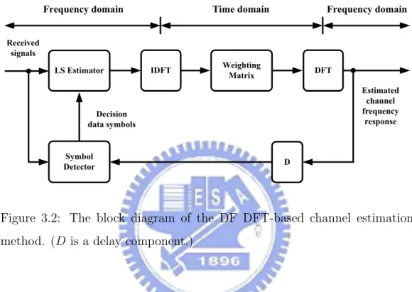
In the second part, we derive the decision-feedback (DF) discrete Fourier transform (DFT)-based channel estimation method from Newton’s method for STBC-OFDM systems. Through our derivation, the equivalence between Newton’s method and the DF DFT-based method is established. Computer simulations are also used to demonstrate the equivalence of the two methods in terms of bit error rate (BER) and normalized square error (NSE) perfor-mance. Finally, the results presented in this part also hold for conventional OFDM systems.

In the third part, we investigate channel estimation for OFDM systems with STBC in mobile wireless channels. Our proposed method consists of two-stage processing and is developed on the basis of the classical DFT-based channel estimation method. In the initialization stage, we employ a multipath interference cancellation (MPIC) technique to estimate multipath delays and multipath complex gains. In the tracking stage, we develop a refined DF DFT-based channel estimation method in which a few pilot tones inserted in OFDM data symbols are applied to form an optimal gradient vec-tor at the first iteration such that the error propagation effect is mitigated. In order to reduce computational complexity, an approximate weighting matrix is adopted to avoid matrix inversion. We demonstrate the proposed method

through computer simulation of an STBC-OFDM system with two transmit antennas and a single receive antenna. The results show that our method out-performs the classical DFT-based method, the STBC-based minimum mean square error (MMSE) method, and the Kalman filtering method as well, and that significant signal-to-noise ratio (SNR) performance improvement can be achieved, especially when a high-level modulation scheme, e.g. 16-quadrature amplitude modulation (QAM), is adopted in low-mobility environments.

In the final part, we resort to the expectation-maximization (EM) al-gorithm to tackle the inter-carrier interference (ICI) problem, caused by time-variant multipath channels, for both the OFDM systems and the bit-interleaved coded modulation (BICM)-OFDM systems. We first analyze the ICI in frequency domain with a reduced set of parameters, and following this analysis, we derive an EM algorithm for maximum likelihood (ML) data detection. An ML-EM receiver for OFDM systems and a TURBO-EM receiver for BICM-OFDM systems are then developed to reduce computa-tional complexity and to exploit temporal diversity, the main idea of which is to integrate the proposed EM algorithm with a groupwise ICI cancellation method. Compared with the ML-EM receiver, the TURBO-EM receiver fur-ther employs a soft-output Viterbi algorithm (SOVA) decoder to exchange information with a maximum a posteriori (MAP) EM detector through the turbo principle. Computer simulation demonstrates that the two proposed receivers clearly outperform the conventional one-tap equalizer, and the per-formance of the TURBO-EM receiver is close to the matched-filter bound even at a normalized maximum Doppler frequency up to 0.1.

Acknowledgements

I would like to express sincere gratitude to my advisor, Dr. Chia-Chi Huang, for his constant support and gracious guidance throughout my re-search works. His constructive suggestion and persistent help enables me to complete my dissertation successfully. I would also thank him for his encouragement to me in many times of frustration.

A debt of gratitude is owed to my colleagues and friends in Wireless Com-munication Laboratory at National Chiao Tung University. Many thanks are due to Dr. Chih-Min Yu, Dr. Shin-Yuan Wang, Dr. Shiang-Jiun Lin, Yong-Ting Chen, Chia-Hui Lin, Shin-Yi Tu as well as other colleagues for providing their invaluable help and consultation in many aspects during my PhD course. A special thanks to Yunn-Wen Chen, Ching-Kai Li, Che-Fang Yeh, Wen-Chuan Chen and Siao-Yi Jhong for their active contribution to my research works. Working with them has been a pleasant and memorable experience.

I would like to express my appreciation to Professors Wen-Rong Wu, Chin-Liang Wang, Shyh-Jye Jou, Sau-Gee Chen, Jeng-Kuang Hwang and Jia-Chin Lin, for their time and very useful comments on improving this dissertation.

Finally, yet importantly, this dissertation is dedicated to my lovely family. I am deeply indebted to my parents, my brother and my sister for their understanding, patience, and unwavering love.

Meng-Lin Ku Hsinchu, Taiwan

Contents

Chinese Abstract i

Abstract iii

Acknowledgements vi

Contents vii

List of Tables xii

List of Figures xiii

Acronyms xvii

Symbols xxi

1 Introduction 1

1.1 Problem and Motivation . . . 4 1.2 Organization of the Dissertation . . . 10 2 A Complementary Codes Pilot-Based Transmit Diversity

2.1 Literature Survey and Motivation . . . 12

2.2 CC Pilot Signals for Two Transmit Antenna Systems . . . 14

2.3 CC Pilot-Based STBC-OFDM Systems: Transmitter Archi-tecture . . . 17

2.4 CC Pilot-Based STBC-OFDM Systems: Receiver Architecture 18 2.4.1 Fine Data Detection . . . 21

2.4.2 Channel Estimation . . . 22

2.4.3 Computational Complexity . . . 24

2.5 Performance Analysis . . . 24

2.5.1 Time-Varying Effect of Two-Path Channels . . . 24

2.5.2 Performance Analysis of Coarse Data Detection . . . . 26

2.5.3 Performance Analysis of Channel Estimation and Fine Data Detection . . . 28

2.6 Computer Simulation . . . 32

2.6.1 Effect of Vehicle Speed . . . 34

2.6.2 Effect of Path Selection . . . 34

2.6.3 Analytic and Simulated BER Performance . . . 35

2.7 Summary . . . 39

3 On the Equivalence between DF DFT-based Channel Esti-mation Method and Newton’s Method in OFDM Systems 40 3.1 Literature Survey and Motivation . . . 40

3.2 STBC-OFDM Systems . . . 41

3.3 DF DFT- Based Method and Newton’s Method . . . 43

3.3.2 Channel Estimation via Newton’s Method . . . 44

3.3.3 Equivalence between Newton’s Method and DF DFT-Based Method . . . 49

3.4 Computer Simulation . . . 54

3.4.1 BER Performance . . . 54

3.4.2 NSE Performance . . . 54

3.5 Summary . . . 58

4 A Refined Channel Estimation Method for STBC-OFDM Systems in Low-Mobility Wireless Channels 59 4.1 Literature Survey and Motivation . . . 59

4.2 STBC-OFDM Systems . . . 62

4.2.1 Transmitted Signals . . . 62

4.2.2 Channel Model . . . 65

4.2.3 Received Signals . . . 65

4.3 Proposed Channel Estimation Method . . . 66

4.3.1 Initialization Stage: The MPIC-Based Decorrelation Method . . . 66

4.3.2 Equivalence between DF DFT-Based Method and New-ton’s Method . . . 69

4.3.3 Refined DF DFT-Based Channel Estimation . . . 71

4.4 Computational Complexity . . . 75

4.5 Computer Simulation . . . 76

4.5.1 NSE Performance of MPIC-Based Decorrelation Method 80 4.5.2 BER Performance . . . 81

4.5.3 Effect of Normalized Maximum Doppler Frequency . . 82

4.5.4 Effect of Number of Pilot Tones . . . 82

4.5.5 Effect of Number of Data Subcarriers Used . . . 83

4.5.6 Average Number of Iterations . . . 83

4.6 Summary . . . 93

5 EM-based Iterative Receivers for OFDM and BICM-OFDM Systems in Doubly Selective Channels 94 5.1 Literature Survey and Motivation . . . 94

5.2 System Model . . . 98

5.2.1 Transmitted and Received Signals . . . 98

5.2.2 Modeling of ICI in Frequency Domain . . . 100

5.3 EM-based Data Detection Method . . . 102

5.4 Implementation: EM-based Iterative Receivers . . . 106

5.4.1 ML-EM Receiver for OFDM Systems . . . 106

5.4.2 TURBO-EM Receiver for BICM-OFDM Systems . . . 112

5.4.3 Initial Setting and Channel Estimation Update . . . . 114

5.4.4 Computational Complexity . . . 115

5.5 Computer Simulation . . . 116

5.5.1 BER Performance of ML-EM Receiver . . . 118

5.5.2 Effect of Group Size . . . 120

5.5.3 BER Performance of TURBO-EM Receiver . . . 120

5.5.4 FER Performance of TURBO-EM Receiver . . . 121

5.6 Summary . . . 128

Bibliography 131

Appendices 143

A Complementary Sequences 143 B Proof of (2.37) and (2.38) 146

C Proof of (3.21) 148

D Explanation of Hessian Matrix 149 E Review of EM Algorithm 151 F Proof of (5.24) and (5.25) 154 G Calculation of (5.36) 156

Vita 157

List of Tables

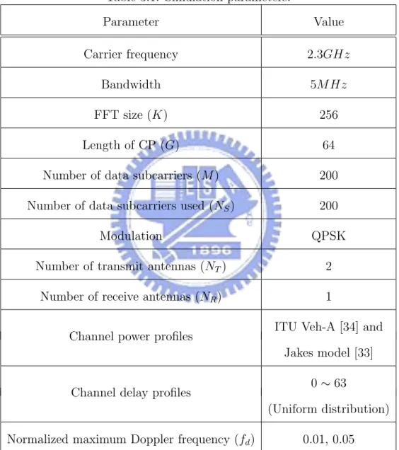
2.1 Simulation parameters. . . 33 3.1 Simulation parameters. . . 55 4.1 Computational complexity for the system parameters given in

Section 4.5. . . 77 4.2 Simulation parameters. . . 78 5.1 Computational Complexity (Ex: G = 4, Q = 4, γ = 1, and

L = 6). . . 117

List of Figures

1.1 Transmitter of basic OFDM systems. . . 5 1.2 Receiver of basic OFDM systems. . . 7 2.1 Transmitter architecture of CC pilot-based STBC-OFDM

sys-tems. . . 19 2.2 Receiver architecture of CC pilot-based STBC-OFDM systems. 19 2.3 Fine data detection functional block. . . 21 2.4 Channel estimation functional block. . . 22 2.5 BER performance versus number of iterations at Eb/σn2=24dB

and fDTs=0.0111. . . 31

2.6 BER performance of CC pilot-based STBC-OFDM systems in the two-path fading channel with vehicular speed as a param-eter (Np = 2). . . 36

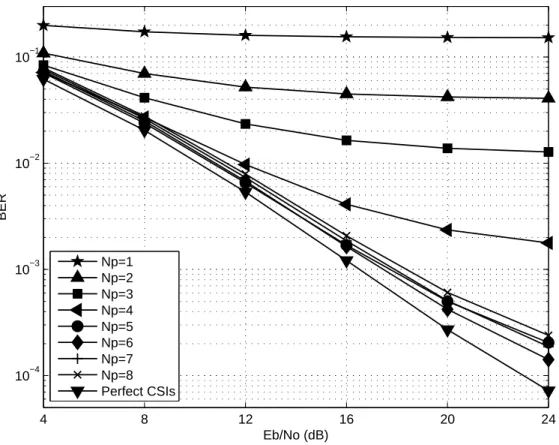
2.7 BER performance of CC pilot-based STBC-OFDM systems in the UMTS system defined fading channel with Np as a

2.8 The analytic and simulated BER performance of CC pilot-based STBC-OFDM systems in the two-path fading channel

with vehicular speed as a parameter. . . 38

3.1 STBC-OFDM systems. . . 42

3.2 The block diagram of the DF DFT-based channel estimation method. (D is a delay component.) . . . 44

3.3 Equivalence between (a) Newton’s method and (b) the DF DFT-based method. . . 53

3.4 BER performance of the two methods. . . 56

3.5 NSE performance of the two methods (fd= 0.05). . . 57

4.1 (a) STBC-OFDM system (b) OFDM frame format. . . 63

4.2 The MPIC-based decorrelation method in the initialization stage. (G is the ratio of the CP length to the useful OFDM symbol time, and IDF T {·} is a K-point IDFT operation.) . . 67

4.3 Block diagram of the refined DF DFT-based channel estima-tion method in the tracking stage. (The subscript ”p” is to indicate that the calculation is only associated with the pilot subcarrier set.) . . . 72

4.4 NSE performance of the MPIC-based decorrelation method in the initialization stage (ve = 240km/hr). . . 84

4.5 BER performance for QPSK modulation in the two-path chan-nel at ve = 240km/hr (|J| = 8 and |Θ| = |Q| = 192). . . 85

4.6 BER performance for 16QAM modulation in the two-path channel at ve = 240km/hr (|J| = 8 and |Θ| = |Q| = 192). . . . 86

4.7 BER performance for 16QAM modulation in the ITU Veh-A channel at ve = 240km/hr (|J| = 8 and |Θ| = |Q| = 192). . . . 87

4.8 BER versus normalized maximum Doppler frequency in the ITU Veh-A channel for QPSK modulation (|J| = 8, |Θ| =

|Q| = 192, and Eb/No=16dB). . . 88

4.9 BER versus normalized maximum Doppler frequency in the ITU Veh-A channel for 16QAM modulation (|J| = 8, |Θ| =

|Q| = 192, and Eb/No=22dB). . . 89

4.10 BER versus number of pilot tones used in the ITU Veh-A channel for 16QAM modulation (ve = 240km/hr, |Θ| = |Q|,

and Eb/No=20dB). . . 90

4.11 BER versus number of data subcarriers used in the ITU Veh-A channel for 16QVeh-AM modulation (ve = 240km/hr, |J| = 8,

and Eb/No=20dB). . . 91

4.12 Average number of iterations versus |Θ| in the ITU Veh-A channel for 16QAM modulation (ve = 240km/hr, |J| = 8,

and Eb/No=20dB). . . 92

5.1 BICM-OFDM systems. . . 98 5.2 EM-based data detection method. . . 107 5.3 (a) ML-EM receiver for OFDM systems (b) An illustration for

group detection. . . 108 5.4 TURBO-EM receiver for BICM-OFDM systems. . . 111 5.5 Initialization procedure for ML-EM and TURBO-EM receivers.114

5.6 BER performance of the ML-EM receiver in the two-path channel (NM L = 3 and [G, Q] = [4, 4]). . . 122

5.7 BER performance of the ML-EM receiver in the ITU Veh-A channel (NM L = 3 and [G, Q] = [4, 4]). . . 123

5.8 BER performance of the ML-EM receiver with channel esti-mation update for various [G, Q] (NM L= 3). . . 124

5.9 BER performance of the TURBO-EM receiver in the two-path channel (NT B = 3 and [G, Q] = [4, 4]). . . 125

5.10 BER performance of the TURBO-EM receiver in the ITU Veh-A channel (NT B = 4 and [G, Q] = [4, 4]). . . 126

5.11 FER performance of the TURBO-EM receiver in the ITU Veh-A channel (NT B = 4 and [G, Q] = [4, 4]). . . 127

Acronyms

• 1G : first-generation

• 2G : second-generation

• 3G : third-generation

• 3GPP : Third Generation Partnership Project

• 4G : fourth-generation

• AR : autoregressive

• AWGN : additive white Gaussian noise

• BER : bit error rate

• BICM : bit-interleaved coded modulation

• BPSK : binary phase-shift keying

• CC : complementary codes

• CDMA : code division multiple access

• CP : cyclic prefix

• CSI : channel state information

• DF : decision-feedback

• DFT : discrete Fourier transform

• ECLL : expected complete log-likelihood

• EM : expectation-maximization

• FER : frame error rate

• FFT : fast Fourier transfom

• GI : guard interval

• GSM : Global System for Mobile Communications

• IAI : inter-antenna interference

• ICI : inter-carrier interference

• IDFT : inverse discrete Fourier transform

• IFFT : inverse fast Fourier transfom

• ISI : inter-symbol interference

• ITU : International Telecommunication Union

• LLR : log-likelihood ratio

• LTE : Long-Term Evolution

• MAP : maximum a posteriori

• MC : multicarrier modulation

• MIMO : multiple-input multiple-output

• ML : maximum likelihood

• MMSE : minimum mean square error

• MPIC : multipath interference cancellation

• MSE : mean square error

• NSE : normalized square error

• OFDM : orthogonal frequency division multiplexing

• OFDMA : orthogonal frequency division multiple access

• P/S : parallel-to-serial

• PAPR : peak-to-average power ratio

• QAM : quadrature amplitude modulation

• QPSK : quadratic phase shift keying

• S/P : serial-to-parallel

• SC : single-carrier

• SM : spatial multiplexing

• SNR : signal-to-noise ratio

• SOVA : soft-output Viterbi algorithm

• STBC : space-time block code

• STC : space-time coding

• TDMA : time division multiple access

• UMTS : Universal Mobile Telecommunications System

• WCDMA : wideband code division multiple access

• WiMAX : Worldwide Interoperability for Microwave Access

Symbols

By convention, boldface letters are used for matrices, vectors, and sets. The superscripts (·)∗_{, (·)}T_{, (·)}H _{and (·)}−1 _{stand for complex conjugate, transpose,}

Hermitian, matrix inversion, respectively. The notation <e(·) takes the real part of (·). The notation IN presents an N × N identity matrix. We deonte

the Kronecker delta function as δ[n]. Besides, we denote the dimension of the vector x as |x|. The notation {·} denotes a set, e.g. a set x = {x1, . . . , x|x|},

where |x| is cardinality of the set x. Further, diag{x} denotes the diagonal matrix with vector x on the diagonal, and diag{X1, . . . , XM} denotes the

block diagonal matrix with the submatrices X1, . . . , XM on the diagonal.

The notations E [·] and Var [·] denote the calculation of expectation and variance, respectively. Finally,  = √−1.

Chapter 1

Introduction

The second-generation (2G) wireless systems were introduced in the early 1990s, and considered as the prominent evolution of cellular systems in telecommunication. Because 2G systems feature the implementation of digi-tal technology, they offer better voice quality and elementary data service, as compared with analog communication provided in the first-generation (1G) radio systems. Today, the European digital cellular system, referred to as Global System for Mobile Communications (GSM), is undoubtedly the most successful 2G systems in the world, and still dominates the cellular service market with over 250 million subscribes in about 120 countries. With the in-creasing demands for multimedia-level data rates in mobile communication, the third-generation (3G) systems, based on wideband code division multiple access (WCDMA) radio technology, are now being progressively deployed on a large scale all over the world. The 3G systems upgrade the existing 2G network to provide data rates up to 144kb/s for high-mobility environments, 284kb/s for low-mobility environments and 2Mb/s for stationary

environ-ments, and they also aim to greatly expand cell coverage. A comprehensive introduction of air interface evolution for cellular communication systems can be referred to [1] for details. A desire for high data rate transmission moti-vates the development of the fourth-generation (4G) systems. In order to get richer multimedia services in the future, the 4G systems attempt to provide a peak data rate up to a level of 100Mb/s for wide area coverage with high mobility and 1Gb/s for local area coverage with low mobility. As data rate increases, the effect of time dispersion in wireless channels becomes much more significant and will cause more severe inter-symbol interference (ISI). As a result, a relatively complicate time-domain equalizer in single-carrier (SC) systems, such as GSM, is needed, which will raise the cost of imple-mentation. In 3G systems, although a rake receiver can be used to combat dispersive fading by resolving and combining the multipath, the receiver is not suitable over a broadband channel due to the appearance of excessive multipath interference. On the other hand, orthogonal frequency division multiplexing (OFDM) is an attractive choice to meet the requirement for high-data-rate transmission in future 4G systems due to its inherent ability to compensate for multipath fading [2]. OFDM was originally proposed in the 1970s, and it is a special form of multicarrier modulation (MC) scheme in which a large number of narrowband and orthogonal subcarriers are used to transmit data symbols in parallel through the use of inexpensive inverse fast Fourier transfom (IFFT) and fast Fourier transform (FFT). As a conse-quence, it converts a frequency selective fading channel into several flat fad-ing channels, and allows for a simpler one-tap equalizer at the receiver side.

Besides, the flexibility of OFDM enables the use of frequency-domain adap-tation and multi-antenna solutions. Based on all these advantages, OFDM has been chosen as a potential air interface candidate for two popular 4G cellular systems [3–5]:

• Worldwide Interoperability for Microwave Access (WiMAX) systems in

IEEE 802.16 standard.

• Long-Term Evolution (LTE) of 3G systems in Third Generation

Part-nership Project (3GPP).

The capacity of wireless communication can be substantially boosted if a communication system employs multiple antennas at the transmitter and receiver, also known as multiple-input multiple-output (MIMO) system. It is proved in [6] that, the capacity of MIMO systems is linearly increased with the minimum number of transmit and receive antennas in a flat fading channel. In order to improve cell coverage and data rate, various MIMO tech-nologies should be supported as a well-integrated part of 4G systems, rather than just an add-on to the specifications [7,8]. Since OFDM is well suited for MIMO processing, the combination of MIMO and OFDM is a nature choice for wideband transmission to obtain diversity gains or multiplexing gains in the spatial dimension. With this popularity, MIMO-OFDM technology has been adopted in several standards, and it is the most attractive air in-terface for high performance 4G broadband wireless communications [9, 10]. The primary goal of this dissertation is to deal with channel estimation and data detection for OFDM systems, and detailed descriptions of problem and motivation are given in the next section.

1.1

Problem and Motivation

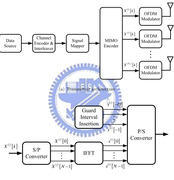
Figure 1.1 shows a transmitter of basic OFDM systems with NT transmit

antennas. The information bits are first encoded by a channel encoder and fed into an interleaver in order to achieve good coding gains as well as di-versity gains. Afterwards, the coded bit stream is mapped onto constellation points, e.g. quadratic phase shift keying (QPSK) or quadrature amplitude modulation (QAM), using a signal mapper, and then processed by an MIMO encoder. The MIMO encoder transforms a symbol stream into NT parallel

substreams, and it can be implemented in a number of different ways, de-pending on application requirements. Herein, we focus on two key schemes: space-time coding (STC) and spatial multiplexing (SM). More details on these two schemes can be found in [11]. In the STC scheme, the same symbol stream is encoded into different substreams across multiple transmit anten-nas to achieve spatial diversity gains. Of particular interest is Alamouti’s space-time block code (STBC) in two transmit-antenna systems [12]. On the other hand, the SM scheme aims at increasing data rate by spatially multiplexing a symbol stream into independent substreams across transmit antennas. After the MIMO processing, these substreams are simultaneously transmitted using the corresponding antennas through the same process of OFDM transmission. As illustrated in Figure 1.1(b), in an OFDM modula-tor at the ith transmit antenna, a symbol substream©X(i)_[k]ª_{is first passed}

through a serial-to-parallel (S/P) converter, and modulated by an inverse fast Fourier transform (IFFT) to produce time domain samples ©x(i)_[n]ª_.

inter-( )1_{[ ]} X k ( )2_{[ ]} X k ( )NT _{[ ]} X k

(a) Transmitter architecture

( )

_{[ ]}

0 i X ( )i

_[

₁

_]

X N− ( )

_{[ ]}

0 i x ( )i

_[

₁

_]

x N− ( )i

_{[ ]}

X k ( )

_{[ ]}

1 i x − ( )i

_{[ ]}

x −G (b) OFDM modulator

val (GI) x(i)_{[n], for n = −1, . . . , −G, with length longer than delay spread, is}

attached at the beginning of these samples through a parallel-to-serial (P/S) converter to generate an OFDM symbol. Although a silent GI can be used to take care of ISI, inter-carrier interference (ICI) remains a critical issue due to the loss of orthogonality among subcarriers. If a cyclic prefix (CP) is used for the GI, ICI can also be avoided. In this regard, the CP is more widely adopted in current standards, and an OFDM symbol transmitted from the

ith antenna is given by

x(i)[n] = 1

N

N −1_X k=0

X(i)[k] e2πknN (1.1)

for n = −G, . . . , N − 1. The impulse response of wireless channels between the ith transmit antenna and the jth receive antenna can be expressed as

h(j,i)[n, τ ] =

L−1

X

l=0

h(j,i)[l, n] δ [τ − l] (1.2)

where h(j,i)_{[l, n] is complex gain of the lth path, associated with path delay}

l, and L is the number of propagation paths. Note that h(j,i)_{[l, n] changes}

with time index n when Doppler spread exists.

The receiver of basic OFDM systems with NRreceive antennas is shown in

Figure 1.2. The received signal at the jth receive antenna can be represented as r(j)[n] = NT X i=1 L−1 X l=0 h(j,i)[l, n] x(i)[((n − l))_N] + z(j)[n] (1.3) where ((·))_N represents modulo N operation and z(j)_{[n] is complex additive}

white Gaussian noise (AWGN) at the jth antenna. At the receiver side, after S/P conversion, GI removal and FFT operation, the received signal of each

( )1_{[ ]} R k ( )2_{[ ]} R k ( )NR _{[ ]} R k ( )1_{[ ]} r n ( )2_{[ ]} r n ( )NR _{[ ]} r n

(a) Receiver architecture

( )j

_{[ ]}

₀ R ( )

_[

_]

1 j R N− ( )

_{[ ]}

0 j r ( )

_[

_]

1 j r N− ( )j

_{[ ]}

R k ( )j

_{[ ]}

₁ r − ( )j

_{[ ]}

r −G (b) OFDM demodulator

antenna arm is transformed into frequency domain as follows:

R(j)_{[k] =} N −1_X

n=0

r(j)_{[n] e}−2πkn_{N (1.4)}

for k = 0, . . . , N −1. By substituting (1.1) and (1.3) into (1.4), we can obtain

R(j)[k] = NT X i=1 L−1 X l=0 N −1_X m=0 X(i)[m] α(j,i)[k, m, l] e−2πmlN + Z(j)[k] (1.5)

where Z(j)_{[k] and α}(j,i)_{[k, m, l] can be evaluated by}

Z(j)_{[k] =} N −1_X n=0 z(j)_{[n] e}−2πkn_{N (1.6)} α(j,i)_{[k, m, l] =} 1 N N −1 X n=0 h(j,i)_{[l, n] e}−2πn((k−m))N_{N (1.7)} We then define H(j,i)_{[k, m] =} L−1 X l=0 α(j,i)_{[k, m, l] e}−2πml N (1.8)

and rewrite (1.5) as follows:

R(j)_{[k] = H}(j,q)_{[k, k] X}(q)_[k] | {z } desired term + NT X i=1,i6=q H(j,i)[k, k] X(i)[k] | {z } IAI term + NT X i=1 N −1_X m=0,m6=k H(j,i)[k, m] X(i)[m] | {z } ICI term + Z(j)_[k] | {z } noise term (1.9)

It is observed from (1.9) that for detecting the qth transmitted signal X(q)_[k],

the demodulated signal R(j)_{[k] suffers from not only noise but also}

inter-carrier interference (ICI) as well as inter-antenna interference (IAI). Essen-tially, the ICI arises from Doppler spread, while the IAI is due to multiple antennas transmission, and these two unwanted signals will severely degrade the performance of a mobile OFDM receiver. When wireless channels are quasi-static, i.e. channel gains are time-invariant, (1.7) and (1.8) become as

α(j,i)_{[k, m, l] =}    h(j,i)_{[l] , for k = m} 0, for k 6= m (1.10) H(j,i)_{[k, m] =}      L−1_P l=0 h(j,i)_{[l] e}−2πml_{N , for k = m} 0, for k 6= m (1.11) where h(j,i)_{[l, n] is a constant value of h}(j,i)_{[l], for n = 0, . . . , N − 1. Then,}

(1.9) is reduced to R(j)_{[k] = H}(j,q)_{[k, k] X}(q)_[k] | {z } desired term + NT X i=1,i6=q H(j,i)_{[k, k] X}(i)_[k] | {z } IAI term + Z(j)_[k] | {z } noise term (1.12) Moreover, the extension of (1.9) and (1.12) to single-input single-output (SISO)-OFDM systems is also straightforward by setting NT = 1 and NR=

1. As expected, there is no IAI problem in this special case.

There are several challenges in attempts to design an OFDM system. As depicted in Figure 1.2, the success of implementing a receiver hinges on

several basic issues, consisting of synchronization, channel estimation, data detection, and channel decoding, etc. In this dissertation, we will focus on channel estimation and data detection problem. From the aforementioned discussion, the knowledge of channel state information (CSI) is required for coherent data detection in (1.9) and (1.12). Hence, it is crucial to have accu-rate estimates of CSI, which is in general difficult to achieve over fast fading channels and MIMO channels. In fast fading channels, a more sophisticated receiver is needed to track rapid channel variation; otherwise, performance deterioration may occur. In MIMO channels, the intent to identify multi-ple channel parameters at each receiver antenna makes channel estimation more challenging. In addition to channel estimation, it is also necessary to investigate data detection for efficiently dealing with ICI and IAI. These ob-servations motivate us to investigate channel estimation and data detection for OFDM systems.

1.2

Organization of the Dissertation

The rest of this dissertation is organized as follows. In Chapter 2, we use complementary codes (CC) to design pilot signals with minimum peak-to-average power ratio (PAPR) for channel estimation in MIMO systems. Then, we present a CC pilot-based STBC-OFDM system which transmits CC pilot signals together with OFDM data signals in time domain without sacrificing bandwidth efficiency. A complete receiver architecture for channel estimation and data detection is proposed and analyzed. Chapter 3 introduces a classical decision-feedback (DF) discrete Fourier transform (DFT)-based channel

es-timation method for STBC-OFDM systems. We then prove the equivalence between the DF DFT-based method and the Newton’s method, and establish their relationship. In Chapter 4, we propose a two-stage channel estimation method for STBC-OFDM systems. In the initialization stage, a multipath interference cancellation (MPIC)-based decorrelation method is employed to identify significant channel taps. Through the equivalence discussed in Chap-ter 3, we develop a refined DF DFT-based channel estimation method in the tracking stage to improve bit error rate (BER) performance. Chapter 5 presents two expectation-maximization (EM)-based iterative receivers to mitigate ICI, introduced by Doppler effect, for both OFDM systems and bit-interleaved coded modulation (BICM)-OFDM systems. We derive an EM algorithm for maximum likelihood (ML) data detection. Towards the goal of reducing computational complexity, we then develop an ML-EM receiver for OFDM systems and a TURBO-EM receiver for BICM-OFDM systems. Chapter 6 draws some conclusions.

Chapter 2

A Complementary Codes

Pilot-Based Transmit Diversity

Technique for OFDM Systems

2.1

Literature Survey and Motivation

In a recent paper, STBC [12, 13] has been suggested to improve the per-formance of an OFDM system [14]. Garg studied the degradation in the performance of the STC with imperfect channel estimation [15]. In general, channel estimation is an important issue in realizing a successful STBC-OFDM system. We all know that channel estimation can be performed at a receiver by inserting pilot signals into transmitted signals. There are sev-eral factors which have to be considered for the practical use of pilot signals in multiple transmit antenna systems. First, pilot signals should be sent in the same frequency band and at the same time with data signals to ensure the accuracy of channel estimation. Second, multiple CSIs must be derived

from the received signal in a system with multiple transmit antennas. To estimate multiple channels, antennas at the transmitter side can alternately transmit a single pilot signal or simultaneously transmit different pilot signals which have impulse-like auto-correlation and zero cross-correlation proper-ties [16–19]. Third, the length of pilot signals should not be too short in order to achieve accurate channel estimation. In some special cases, pilot signals take the length of 2P_{, where P is an integer, to meet with the requirement of}

fast signal processing algorithms. Finally, the values of pilot signals need to be taken from some predetermined signal sets such as {1, −1, , −} to main-tain constant amplitude and avoid the non-linear effect of an amplifier. The design of optimal pilot signals is an open problem [16–23]. Computer simu-lations are used in [16–19] to exhaustively search the pilot signals which are able to achieve MMSE channel estimation. [20] proposed a channel estimator based on the correlation of channel frequency response at adjacent frequen-cies. However, a large size of matrix inverse is required in this scheme. [21–23] extended the work in [20] to reduce the complexity of channel estimation. Besides, some channel estimation methods based on superimposed training sequences are proposed for SISO-OFDM systems [24–26]. At the expense of reducing power efficiency, these methods can not only significantly save bandwidth but also effectively track time-variant channels. Recently, chan-nel estimation using superimposed training for MIMO-OFDM systems has been investigated [27, 28]. The PAPR of the OFDM signals with superim-posed training is analyzed in [29], and it is demonstrated that the constant magnitude pilot sequences result in the best BER performance due to their

ability to lower the PAPER of the transmitted OFDM signal.

In this chapter, we suggest that CC can be used as pilot signals and transmitted in time domain for the purpose of channel estimation in a two transmit antenna system. The CC pilot signals satisfy the requirements of pilot signals we mentioned above, and at the same time, have the minimum PAPR. We will describe the functional block diagrams and simulate the per-formance of an STBC-OFDM system with CC pilot signals. The rest of this chpater is organized as follows. In Section 2.2, we will describe the CC pilot signals for a two transmit antenna system. In Section 2.3, We will introduce the transmitter architecture of a CC pilot-based STBC-OFDM system. The details of the receiver operation such as data detection, channel estimation, etc., are described in Section 2.4. The performance of the CC pilot-based STBC-OFDM system is then analyzed in Section 2.5. In Section 2.6, we show our computer simulation and performance evaluation results. Finally, concluding remarks are drawn in Section 2.7.

2.2

CC Pilot Signals for Two Transmit

An-tenna Systems

Binary CC was originally conceived by Golay for infrared multi-slit spec-trometry applications [30, 31]. More recently, these codes were also used in OFDM systems to reduce PAPR [32]. For details, please refer to Appendix A. We can define CC as follows. Let us consider a pair of equally long se-quences {α [n]} and {β [n]}, for n = 0, . . . , N − 1, where N is the length of the two sequences. These sequences are called CC if their auto-correlations

satisfy the relationship: Γ [n] ≡ N −1_X m=0 {α [m] α∗_{[((m − n))} N] + β [m] β∗[((m − n))_N]} = 2N · δ [n] =    2N, for n = 0 0 , for n 6= 0 (2.1) where (·)∗ _{denotes the complex conjugate operation, ((·))}

N denotes the

mod-ulo N operation, and δ[n] is the Kronecker delta function.

The pilot signals of a two transmit antenna system can be constructed from a pair of CC. For simplicity, we assume that CC sequences {α [n]} and {β [n]} are normalized such that their combined auto-correlation value Γ [n] = δ [n] as shown in (2.1). Consider a system with two transmit anten-nas and one receive antenna. Two signals {α [n]} and {−β [n]} are simulta-neously transmitted from the two transmit antennas over two independent frequency selective fading channels in the first time slot; the other two signals

{β∗_[((−n))

N]} and {α∗[((−n))N]} are then simultaneously transmitted over

the same two channels in the second time slot. Furthermore, a CP is added before each transmitted pilot signal to avoid ISI and to preserve the circular convolution between the pilot signal and the channel impulse response in the time domain. Here, we assume that the two channels are quasi-static over the two transmission time slots. Hence, the received pilot signals in the fre-quency domain in the first and second time slot, RT 1[k] and RT 2[k], can be

expressed as  RT 1[k] RT 2[k]   =  Pα[k]−Pβ[k] P∗ β[k] Pα∗[k]    H1[k] H2[k]   + Z [k] = P [k]  H1[k] H2[k]   + Z [k] (2.2) for k = 0, . . . , N − 1, where H1[k] and H2[k] are the channel frequency

responses from the two transmit antennas to the receive antenna, Pα[k] and

Pβ[k] are the N-point DFT of the CC sequences {α [n]} and {β [n]}, P [k]

is called a pilot matrix which is a unitary matrix, and Z [k] is an AWGN vector with zero mean and covariance matrix σ2

nI2, where IK is a K × K

identity matrix. The received pilot signals are then multiplied by a matrix PH_{[k], where (·)}H _{denotes the complex conjugate transpose operation, to}

obtain estimated CSIs in the frequency domain  Hˆ1[k] ˆ H2[k]   = PH _[k]  RT 1[k] RT 2[k]   =  H1[k] H2[k]   + PH_{[k] Z [k] (2.3)}

for k = 0, . . . , N − 1. As a result, the mean square error (MSE) of channel estimation is given by MSE = E ·¯ ¯ ¯ ˆHj[k] − Hj[k] ¯ ¯ ¯2 ¸ = σ2 n, for j = 1, 2 (2.4)

Generally speaking, the pilot matrix can be any unitary matrix which satisfies the power constraint of |Pα[k]|2 + |Pβ[k]|2 = 1 for all k. For

ex-ample, |Pα[k]|2 = |Pβ[k]|2 = 1/2 for all k also satisfies the unitary matrix

requirement. However, the CC pilot signals used in this dissertation have the minimum PAPR (= 0dB) in time domain, thus improve radio frequency power amplifier efficiency. In the case of |Pα[k]|2 = |Pβ[k]|2 = 1/2 for all k,

the PAPR is 10logN (dB). Moreover, we can easily extend the design of the pilot matrix to four transmit antenna systems by using a 2×2 unitary matrix as follows: P4[k] = 1 √ 2   P [k] P [k] −P [k]P [k]   _(2.5)

2.3

CC Pilot-Based STBC-OFDM Systems:

Transmitter Architecture

The transmitter block diagram of a CC pilot-based STBC-OFDM system is shown in Figure 2.1. The block diagram shows two transmit antennas. The transmitted signal from each antenna consists of a data signal and a pilot signal. Now we describe the generation of the data signals. At the output of the signal mapper, the ith block of 2N data symbols d(i)_{[k] are separated}

into two data sub-blocks and represented as

X_F(i)[k] = d(i)[k] (2.6) and

for k = 0, . . . , N − 1, where N denotes number of subcarriers in an OFDM symbol, X_F(i)[k] and X_S(i)[k] are the kth data symbol of the first and sec-ond data sub-block, respectively. Here, we use Alamouti’s STBC encoding method [12] to encode the two data sub-blocks, X_F(i)[k] and X_S(i)[k], in the sequence as described in [14]. An N-point inverse discrete Fourier transform (IDFT) unit is used in each arm of Figure 2.1 to transform the frequency domain data symbols into a time domain data signal. Afterward, we add the CC pilot signal as described in Section 2.2 to the time domain data sig-nal. Both the data signal and the pilot signal are assumed to be of the same length and they are added synchronously to become an effective OFDM sym-bol with symsym-bol duration T . The cyclic extension with time duration Tg of

an effective OFDM symbol is then inserted as a GI to combat the ISI effect. Finally, a complete OFDM symbol with symbol duration Tsis converted into

an analog signal with a digital-to-analog converter, filtered by a low-pass fil-ter, up converted to radio frequency band, and transmitted in air with a pre-selected antenna, where we set Ts = T + Tg.

2.4

CC Pilot-Based STBC-OFDM Systems:

Receiver Architecture

The receiver block diagram of the CC pilot-based STBC-OFDM system is shown in Figure 2.2. This receiver architecture consists mainly of a fine data detection functional block and a channel estimation functional block, along with other common blocks. After a radio frequency signal is received from an antenna, it is down converted to the equivalent baseband, low-pass filtered,

( )i_{[ ]} F X k ( )i_{[ ]} S X k 2N b bits

Figure 2.1: Transmitter architecture of CC pilot-based STBC-OFDM sys-tems. ( )i_{[ ]} o Y k ( )i[ ] e Y k ( )i_{[ ]} o y n ye( )i[ ]n ( )i_{[ ]} o Y k Ye( )i[ ]k ( )_{[ ]} 1 ˆi H k ˆ2( )[ ] i H k

and digitized. We assume that timing and carrier frequency synchronization are perfect and the length of the channel impulse response is not longer than the length of the GI. The channels are assumed to be quasi-static during any two successive OFDM symbols duration. The frequency response of the propagation channel between the first transmit antenna and the receive antenna is denoted by H₁(i)[k], and the other one is denoted by H₂(i)[k], where index i is used to indicate the corresponding (2i) th and (2i + 1) th OFDM symbol duration. Hence, after the GI removal, S/P conversion and N-point DFT computation, the successively received signals Ye(i)[k] and Yo(i)[k] on

the kth subcarrier in the (2i) th and (2i + 1) th OFDM symbol duration can be represented as Y(i) e [k] = H (i) 1 [k] ³ X_F(i)[k] + Pα[k] ´ +H₂(i)[k] ³ X_S(i)[k] − Pβ[k] ´ + Z(i) e [k] (2.8) and Y(i) o [k] = H (i) 1 [k] ³ −X_S(i)∗[k] + P∗ β [k] ´ +H₂(i)[k] ³ X_F(i)∗[k] + P∗ α[k] ´ + Z(i) o [k] (2.9)

for k = 0, . . . , N − 1, where Ze(i)[k] and Zo(i)[k] are the AWGN in the (2i) th

and (2i + 1) th OFDM symbol duration, respectively. The noise is modeled as an independent complex Gaussian random variable with zero-mean and variance σ2

( )i _{[ ]} o Y k Ye( )i[ ]k ( )i_{[ ]} e Y k ( )i_{[ ]} o Y k ( )i _{[ ]} F X k ( )i _{[ ]} S X k ( )_{[ ]} ˆ i F X k ( )_{[ ]} ˆ i S X k ( )_{[ ]} 1 ˆ i H k ˆ( )2 [ ] i H k

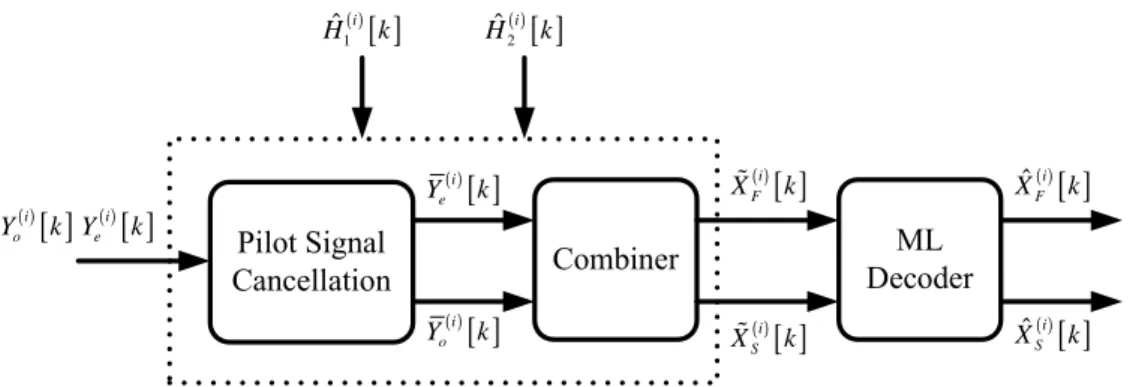
Figure 2.3: Fine data detection functional block.

2.4.1

Fine Data Detection

Figure 2.3 shows the details of the fine data detection functional block which include a pilot cancellation unit, a combiner unit and an ML decoder unit. We assume that the estimated CSIs are accurate, i.e. Hˆ₁(i)[k] = H₁(i)[k];

ˆ

H₂(i)[k] = H₂(i)[k], and the pilot interference signals can thus be reconstructed and be completely subtracted from the received signals Ye(i)[k] and Yo(i)[k].

The output of the pilot signal cancellation unit can be expressed as ¯ Y(i) e [k] = H1(i)[k] XF(i)[k] + H (i) 2 [k] XS(i)[k] + Ze(i)[k] (2.10) and ¯ Y(i) o [k] = −H (i) 1 [k] X (i)∗ S [k] + H (i) 2 [k] X (i)∗ F [k] + Zo(i)[k] (2.11)

for k = 0, . . . , N − 1. We then use the combiner unit to combine the received signals from different transmit antennas according to the method revealed in [14]. Finally, in the ML decoder unit, the ML decision rule can be used to detect the transmitted data symbol on each subchannel [12].

( )i_{[ ]} e Y k ( )i_{[ ]} o Y k ( )_{[ ]} ˆi FC X k XˆSC( )i [ ]k ( )i_{[ ]} e Y k ( )i_{[ ]} o Y k ( )_{[ ]} 1 i h n ( )_{[ ]} 2 i h n ( )_{[ ]} 1 ˆi h n ( )_{[ ]} 2 ˆi h n ( )_{[ ]} 1 ˆi H k ( )_{[ ]} 2 ˆi H k

Figure 2.4: Channel estimation functional block.

2.4.2

Channel Estimation

Figure 2.4 depicts the detailed structure of the channel estimation functional block. First, we use a coarse data detection unit to obtain coarsely estimated data symbols ˆX_{F C}(i) [k] and ˆX_SC(i) [k] by using the estimated CSIs in the previ-ous two OFDM symbols, i.e., the (2i − 2) th and (2i − 1) th OFDM symbol. The structure of the coarse data detection unit is similar to the fine data detection functional block as shown in Figure 2.3. The data interference sig-nals are then reconstructed and subtracted from the received sigsig-nals Ye(i)[k]

and Yo(i)[k] in a data interference cancellation unit. We assume that the data

interference signals can be cancelled perfectly and the refined signals can be represented as

^

Y_e(i)[k] = H₁(i)[k] Pα[k] − H2(i)[k] Pβ[k] + Ze(i)[k] (2.12)

and ^ Y(i)_o [k] = H₁(i)[k] P∗ β [k] + H (i) 2 [k] Pα∗[k] + Zo(i)[k] (2.13)

for k = 0, . . . , N − 1. Next, the refined signals are multiplied by the complex conjugate transpose of the pilot matrix P [k] in the pilot matching unit in Figure 2.4, to obtain more accurately estimated CSIs in the frequency do-main. We then use an N-point IDFT unit to obtain the estimated CSIs in the time domain, i.e.,

¯h(i) 1 [n] = h(i)1 [n] + IDF T © Z_e(i)[k] P_α∗[k] + Z_o(i)[k] Pβ[k] ª (2.14) and ¯h(i) 2 [n] = h(i)2 [n] + IDF T © −Z_e(i)[k] P_β∗[k] + Z_o(i)[k] Pα[k] ª (2.15) for n = 0, . . . , N − 1. Finally, a path selection unit is used to suppress the noise effect and to refine the estimated CSIs. For path selection, we first define a parameter Np, which is the desired number of paths to be selected.

Only the Np paths with larger amplitudes in ¯h(i)1 [n] (or ¯h (i)

2 [n]) are preserved

and all the other paths are discarded. As a result, we obtain ˆh(i)₁ [n] and ˆh(i)

2 [n] in the following way:

ˆh(i) j [n] =    ¯h(i) j [n] , if ¯ ¯ ¯¯h(i)_j [n] ¯ ¯

¯ is one of the Np larger values

0, otherwise

(2.16) for n = 0, . . . , N − 1 and j = 1, 2.

To initialize the channel estimator, pilot preambles without data signals added are transmitted in the first two OFDM symbols. The received signals are passed only through the pilot matching and the path selection unit to generate the preliminary channel estimations.

2.4.3

Computational Complexity

In this subsection, the complexity of the CC pilot-based STBC-OFDM re-ceiver will be calculated in terms of the number of complex multiplications. Either N-point DFT or IDFT needs DF T N multiplications per OFDM sym-bol. At the recever, three DFT or IDFT operations are needed for every OFDM symbol (see Figure 2.2 to Figure 2.4). According to Figure 2.3, the pilot signal cancellation unit and the combiner unit need 8N multiplications for every two OFDM symbols. In Figure 2.4, the data interference cancella-tion unit and the pilot matching unit also need 8N multiplicacancella-tions for every two OFDM symbols. Furthermore, the coarse data detection unit requires the same number of multiplications as the fine data detection functional block, i.e. 8N per two OFDM symbols. Hence, the receiver has the complexity order of 3DF T N + 12N multiplications per OFDM symbol.

2.5

Performance Analysis

In this section, we include an analysis of the BER performance of the pro-posed system in a two-path fading channel. The analysis method is general and can be easily extended to a mobile radio channel with more paths.

2.5.1

Time-Varying Effect of Two-Path Channels

The equivalent baseband impulse response of the two-path fading channel is represented by

where δ [n] denotes a delta function, τ is the excess delay of the second path, and al is the complex gain of the lth path. Assume that the complex gain

of the lth path, for l = 1 and 2, during the (2i) th and (2i + 1) th OFDM symbol is a complex Gaussian random variable and denoted as a(i)_l = a(i)_l,I +

a(i)_l,Q, where a(i)_l,I and a(i)_l,Q are the real and imaginary part of a(i)_l , respectively. According to the Jakes fading channel model [33], the random variables a(i−1)_l,I ,

a(i−1)_l,Q , a(i)_l,I and a(i)_l,Q have the following correlations: E

h

a(i−1)_l,I a(i)_l,I

i = E h a(i−1)_l,Q a(i)_l,Q i = εl 2J0(2πfD(2Ts)) (2.18) and E h

a(i−1)_l,I a(i)_l,Q

i = E

h

a(i−1)_l,Q a(i)_l,I

i

= 0 (2.19) where E [·] is the operation of taking expectation, εl = E

·¯ ¯ ¯a(i)_l ¯ ¯ ¯2 ¸ is the power of the lth path, fD is the maximum Doppler frequency, and J0(·) is the Bessel

function of the first kind. In order to model the time-varying effect of the

lth path between a(i−1)_l and a(i)_l , we have the following equation:

a(i)_l = a(i−1)_l + ∆(i)_l (2.20)

where ∆(i)_l is a complex Gaussian random variable with zero mean. Therefore, the normalized error power of the lth path becomes

E ·¯ ¯ ¯∆(i)_l ¯ ¯ ¯2 ¸ εl = 2 (1 − J0(4πfDTs)) (2.21)

Assume the corresponding channel frequency response is denoted by H(i)_[k],

and as a result, the channel variation in frequency domain, Ω(i)_{[k], can be}

described by the following equation:

The two fading paths are assumed to be independent of each other, and it is obtained from (2.21) that Ω(i)_{[k] is a zero-mean complex Gaussian random}

variable with variance

σ_Ω2 = Eh¯¯Ω(i)[k]¯¯2 i = 2 (1 − J0(4πfDTs)) 2 X l=1 εl (2.23)

Without loss of generality, we assume that the channel power is normalized to one, i.e. P2_l=1εl = 1; hence, we get σ2Ω = 2 (1 − J0(4πfDTs)).

2.5.2

Performance Analysis of Coarse Data Detection

Assume that binary phase-shift keying (BPSK) modulation is used, and data signals X_F(i)[k] and X_S(i)[k] in each subcarrier k are independently and iden-tically distributed (i.i.d.) random variables with zero mean and variance

Eb/2. For the simplicity of analysis, it is assumed that the CC sequences

are ideal random binary sequences with zero mean, and the power of CC pilot signals is the same as data signals. Finally, we assume that the esti-mated CSI ˆH₁(i−1)[k] used by the coarse data detection unit can be modeled as H₁(i)[k] − Λ(i)₁ [k], where the term Λ(i)₁ [k] includes both the effects of chan-nel variation and chanchan-nel estimation error, and its mean and variance are given by zero and σ2

Λ. The estimated CSI ˆH (i−1)

2 [k] is also assumed in a

like manner. For simplicity, the indices i and k are omitted in the following derivation.

From (2.8) and (2.9), the outputs of the pilot signal cancellation unit, in the coarse data detection unit in Figure 2.4, are given by

¯ YeC = H_| 1XF_{z+ H2XS_} De + P_|αΛ1_{z− PβΛ_}2 ˜ Ie +Ze (2.24)

and ¯ YoC = −H_| 1XS∗_{z+ H2XF∗_} Do + P_β∗Λ1+ Pα∗Λ2 | {z } ˜ Io +Zo (2.25)

where ¯YeC and ¯YoC consist of three mutually independent components:

·

desired data signal components De and Do;

·

residual pilot interference signal components ˜Ie and ˜Io;

·

AWGN components Ze and Zo.

Since the random variables Pα, Pβ, Λ1, and Λ2 are mutually independent of

each other, the mean and variance of ˜Ie and ˜Io are given by

E h ˜ Ie i = E h ˜ Io i = 0 (2.26) and Var h ˜ Ie i = Var h ˜ Io i = EbσΛ2 (2.27)

where Var [·] is the operation of taking variance. Given the channel gains H1

and H2, and the transmitted data signals XF and XS, we have the mean

E£Y¯eC

¤

= H1XF + H2XS (2.28)

E£Y¯_oC∗ ¤= −H₁∗XS+ H2∗XF (2.29)

and the variance

Var£Y¯eC

¤

The outputs of the combiner unit in the coarse data detection unit are [14] ˜ XF C = ˆH1∗Y¯eC + ˆH2Y¯oC∗ (2.31) and ˜ XSC = ˆH2∗Y¯eC − ˆH1Y¯oC∗ (2.32) Since ˆH∗

1, ¯YeC, ˆH2 and ¯YoC∗ are mutually uncorrelated of each other, the mean

and variance of ˜XF C are given by

E h ˜ XF C i = E h ˆ H∗ 1 i E£Y¯eC ¤ + E h ˆ H2 i E£Y¯∗ oC ¤ = ζXF (2.33) and Var h ˜ XF C i = E2h_Hˆ∗ 1 i Var£Y¯eC ¤ + E2£_Y¯ eC ¤ Var h ˆ H∗ 1 i +E2h_Hˆ 2 i Var£Y¯∗ oC ¤ + E2£_Y¯∗ oC ¤ Var h ˆ H2 i +Var h ˆ H₁∗ i Var£Y¯eC ¤ + Var h ˆ H2 i Var£Y¯_oC∗ ¤ = ζ¡2EbσΛ2 + σ2n ¢ + 2EbσΛ4 + 2σ2Λσn2 (2.34)

where ζ = |H1|2+ |H2|2. Similarly, the other combiner output ˜XSC has the

same variance as ˜XF C, but different mean ζXS. Therefore, conditioned on

the combined channel gain ζ, the BER is given by

BERC(ζ) = Q µ ζ √ aζ + b ¶ (2.35) where Q (x) = R_x∞¡1±√2π¢e−y2_/2 dy, a = 2σ2 Λ+ σn2/Eb, b = 2σΛ4+ 2σΛ2σn2/Eb.

2.5.3

Performance Analysis of Channel Estimation and

Fine Data Detection

As shown in Figure 2.4, in order to reconstruct the data interference signals, tentative decisions of data symbols are made and denoted as ˆXF C and ˆXSC.

From (2.8) and (2.9), notice that after the data interference cancellation, the output signal Y^e is given by

^ Ye = H_| 1Pα_{z− H2Pβ_} Ie + H1 ³ XF − ˆXF C ´ + Λ1XˆF C + H2 ³ XS − ˆXSC ´ + Λ2XˆSC | {z } ˜ De +Ze (2.36)

and consists of three parts. The first part is the desired pilot signal Ie. The

second part is the residual data interference signal ˜De, which is caused by two

factors. One is the channel estimation error, and the other is the tentative data decision error from the coarse data detection unit. The third part is AWGN Ze. From (2.35) and (2.36), the mean and the second moment of ˜De

can be calculated as (see Appendix B) E h ˜ De i = 2BERC(ζ) (H1XF + H2XS) (2.37) and E ·¯ ¯ ¯ ˜De ¯ ¯ ¯2 ¸ = 2BERC(ζ) ζEb+ σΛ2Eb +4BER2 C(ζ) (H1H2∗XFXS∗+ H1∗H2XF∗XS) (2.38)

Similarly, for the other output Y^o, we have the residual data interference

signal ˜Do as follows E h ˜ Do i = 2BERC(ζ) (−H1XS∗ + H2XF∗) (2.39) and E ·¯ ¯ ¯ ˜Do ¯ ¯ ¯2 ¸ = 2BERC(ζ) ζEb+ σ2ΛEb −4BER2_C(ζ) (H1H2∗XFXS∗ + H1∗H2XF∗XS) (2.40)

According to (2.3) and (2.36), the estimated CSIs at the output of the pilot matching unit can be written as

¯ H1 = H1 + 1 Eb ³ P_α∗D˜e+ Pα∗Ze+ PβD˜o+ PβZo ´ (2.41) and ¯ H2 = H2+ 1 Eb ³ −P∗ βD˜e− Pβ∗Ze+ PαD˜o+ PαZo ´ (2.42) As can be seen in (2.41) and (2.42), the estimated CSIs ¯H1 and ¯H2 have

different means H1 and H2, respectively, but equal variance 2BERC(ζ) ζ +

σ2

Λ+ σn2/Eb. In a two-path fading channel, the variance of ¯H1 and ¯H2 can be

further reduced by a factor of 2/N if we assume the path selection process is perfect, i.e., we have

¯ σ2 Λ= Var £ _¯ H1 ¤ = Var£H¯2 ¤ = 2 N µ 2BERC(ζ) ζ + σ2Λ+ σ2 n Eb ¶ (2.43) We can then replace σ2

Λ with ¯σΛ2 in (2.35) to obtain the BER, denoted as

BER (ζ), for the fine data detection unit. With the two-path Rayleigh

fad-ing channel model, ζ is a random variable with probability density function

p (ζ) = ζe−ζ_{, where ζ ≥ 0. The averaged BER for the fine data detection}

unit can be obtained by averaging BER (ζ) over ζ, i.e.

BER =

Z _∞

0

BER (ζ) p (ζ)dζ (2.44)

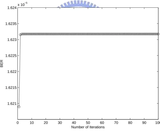
In general, BER can be computed iteratively using software like MATLAB with the following procedure:

1. Initially, we set the variance of channel estimation error in the pilot preambles as σ2

2. Due to the Doppler effect, the variance of channel estimation error for the next two OFDM symbols is given by σ2

Λ= σ2U+ σΩ2

3. Using (2.35), (2.43) and (2.44), we can calculate BERC(ζ), ¯σΛ2, BER (ζ),

and BER, respectively.

For simple analysis of BER performance, we average ¯σ2

Λ over ζ and use the

averaged ¯σ2

Λ instead of σ2U for the next iteration (return to the procedure 2).

With 100 iterations, i.e., 200 OFDM symbols are processed, Figure 2.5 shows that BER almost stayed at the same value.

0 10 20 30 40 50 60 70 80 90 100 1.621 1.6215 1.622 1.6225 1.623 1.6235 1.624x 10 −5 Number of Iterations BER

Figure 2.5: BER performance versus number of iterations at Eb/σn2=24dB

2.6

Computer Simulation

We utilize computer simulations to verify the performance of the proposed CC pilot-based STBC-OFDM system in a two-path fading channel and a Universal Mobile Telecommunications System (UMTS) defined channel. The complex gain of each path is independently generated from the Jakes fading channel model [33]. The relative path power profiles of the two-path channel is 0, 0 (dB). Besides, the channel selected for evaluating the third generation UMTS European systems with relative path power profiles: 2.5, 0, 12.8, -10, -25.2, -16 (dB), is also used to simulate the system performance [34]. We also assume the two transmit antennas are spatially separated far enough and the two channels from the two transmitters to the receiver are uncorrelated in our simulation.

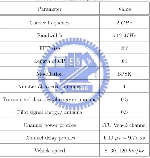
The system parameters for the CC pilot-based STBC-OFDM system sim-ulation are listed in Table 2.1. In our simsim-ulation, a single-user at a time scenario, i.e. time division multiple access (TDMA) can be used as a multi-ple access scheme, is assumed. The entire simulations are conducted in the equivalent baseband. We assume both symbol synchronization and carrier synchronization are perfect. Golay’s binary CC [31] is directly used to gen-erate the CC pilot signals. Each antenna transmits both the data signal and the pilot signal at an equal power level of 0.5 per sample. The excess delay of the paths is uniformly distributed between 0.19µs and 9.77µs. Finally, throughout the simulation, the parameter Eb/No is defined as the received

Table 2.1: Simulation parameters. Parameter Value Carrier frequency 2 GHz Bandwidth 5.12 MHz FFT size 256 Length of CP 64 Modulation BPSK Number of receive antennas 1 Transmitted data signal energy/ antenna 0.5

Pilot signal energy/ antenna 0.5

Channel power profiles ITU Veh-B channel Channel delay profiles 0.19 µs ∼ 9.77 µs