模糊K-最近相鄰點分類法於蛋白質可溶性預測

(1)

國立交通大學

電機與控制工程研究所

碩士論文

模糊

K-最近相鄰點分類法於蛋白質可溶性預測

Fuzzy K-Nearest Neighbor Classifier to Predict Protein

Solvent Accessibility

學生：施逸祥

指導教授：張志永

(2)

模糊

K-最近相鄰點分類法於蛋白質可溶性預測

Fuzzy K-Nearest Neighbor Classifier to Predict Protein

Solvent Accessibility

學生 : 施逸祥 Student : Yi-Xiang Shi

指導教授 : 張志永 Advisor : Jyh-Yeong Chang

國立交通大學

電機與控制工程學系

碩士論文

A Thesis

Submitted to Department of Electrical and Control Engineering

College of Electrical Engineering and Computer Science

National Chiao Tung University

in Partial Fulfillment of the Requirements

for the Degree of Master in

Electrical and Control Engineering

July 2007

Hsinchu, Taiwan, Republic of China

(3)

模糊 K-最近相鄰點分類法於蛋白質可溶性預測

學生:施逸祥指導教授:張志永博士國立交通大學電機與控制工程研究所

摘要

蛋白質在生物體中一直扮演著很重要的角色，蛋白質被發現的數量及其結構逐年增加。隨著蛋白質的應用越來越廣泛，待解決的課題也就越來越多。例如：蛋白質二級結構預測問題、蛋白質相對溶劑可接觸性預測問題等。本篇論文，我們利用修改的模糊K-最近相鄰點法，混合從 PSI-BLAST 產生的位置加權矩陣，針對蛋白質相對溶劑可接觸性預測問題進行研究。最近 Sim 等人 [31]，應用模糊K-最近相鄰點法於蛋白質可溶性預測有顯著的效果。我們提出改進之模糊 K-最近相鄰點法，應用在三態相對溶劑可接觸性預測和二態相對溶劑可接觸性預測，所得到的實驗結果與近幾年的其它方法比較，有較佳的預測正確率。我們並與歐等人 [52]所發表的快速輻射半徑基底函數網路演算法做結合。最後，將這兩種方法之結果做資訊融合以有效地提高預測的準確度。六種修正方法包括:(1) 模糊K-最近相鄰點法、(2) 改進的模糊 K-最近相鄰點法、(3)

(4)

快速輻射半徑基底函數網路演算法、(4) 第一種線性相加合併法、(5) 第二種線性相加合併法、以及(6) 信心指數合併法。在大部分條件表現最佳的情況下，我們建議選擇第二種線性相加合併法。

(5)

Fuzzy K-Nearest Neighbor Classifier to Predict Protein

Solvent Accessibility

STUDENT: YI-XIANG SHI ADVISOR: JYH-YEONG CHANG

Institute of Electrical and Control Engineering National Chiao-Tung University

Abstract

Proteins have been played an important role in a creature and the numbers of proteins and their structures have been increased with years. Since protein applications are more widely used, there will be a lot of problems to be solved.

Using a position-specific scoring matrix (PSSM) generated from PSI-BLAST in this thesis, we develop the modified fuzzy k-nearest neighbor method to predict the protein relative solvent accessibility. By modifying the membership functions of the fuzzy k-nearest neighbor method by Sim et al. [31], has recently been applied to protein solvent accessibility prediction with excellent results. Our modified fuzzy

k-nearest neighbor method is applied on three-state, E, I, and B, and two-state, E, and

B, relative solvent accessibility predictions, and its prediction accuracy compares favorly with those by the fuzzy k-NN and QuickRBF approaches. At last, we combine

(6)

the prediction results of modified fuzzy k-nearest neighbor method and QuickRBF approach to improve the performance. Six modification approaches include: (1) Fuzzy

K-Nearest Neighbor Method, (2) Modified Fuzzy K-Nearest Neighbor Method, (3)

QuickRBF, (4) Linear Combination Fusion 1, (5) Linear Combination Fusion 2, and (6) Reliability Index Fusion. We recommend the Linear Combination Fusion 2 approach which has shown the best performance in most cases.

(7)

Acknowledgement

I would like to express my sincere appreciation to my advisor, Dr. Jyh-Yeong Chang. Without his patient guidance and inspiration during the two years, it is impossible for me to overcome the obstacles and complete the thesis. In addition, I am thankful to all my lab members for their discussion and suggestion.

Finally, I would like to express my deepest gratitude to my family. Without their strong support and encouragement, I could not go through the two years.

(8)

List of Figures

Fig. 2.1. Measure Accessibility……….………….………...19

Fig. 2.2. Binary Model……….……...………….….…………...23

Fig. 2.3. Raw Profile From PSI-Blast Log File………...……...25

Fig. 2.4. BLOSUM 62 Matrix……….….………...25

Fig. 2.5. Simple 2-D case, each instance is described only by two values …...….27

Fig. 2.6. General Architecture of Radial Basis Function Network.…………...31

Fig. 3.1. The two-state membership functions……….……...39

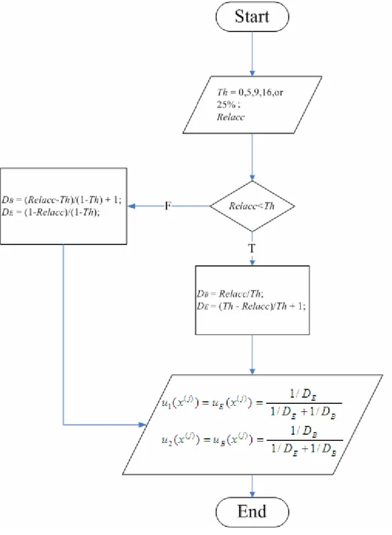
Fig. 3.2. The flowchart to calculate 2-state membership values……….40

Fig. 3.3. The three-state membership functions………..41

Fig. 3.4. The flowchart to calculate 3-state membership values...42

Fig. 3.5. Architecture of QuickRBF method...………....44

Fig. 3.6. The normalization procedure in Linear Combination Fusion 1…………46

(11)

List of Tables

Table 2.1. Database of Non-Homologous Proteins Used For Seven-Fold Cross Validation...17 Table 2.2. Definition of Solvent Accessibility States...21 Table 3.1. Fusion method : Linear combination……….…………...47 Table 4.1. RSA classification accuracy of two kinds Fuzzy K - Nearest Neighbor methods on the RS126 data set with PSI-BLAST pssm profiles……...52 Table 4.2. RSA classification accuracy of QuickRBF and the fusion methods………54 Table 4.3 Comparison of performance of the six approaches in RSA prediction on the RS126 data set with PSSMs generated by PSI-BLAST………...56 Table 4.4. The accuracy tables A of Modified Fuzzy K-NN on each fold and RS126…………...58 Table 4.5. Matthew’s Correlation Coefficients of the five approaches on RS126………60 Table 4.6. Comparison of performance of Modified Fuzzy K-NN approach with other methods…...64

(12)

Chapter 1. Introduction

1.1 Motivation and the Background of this Research

The solvent accessibility of amino acid residues plays an important role in tertiary structure prediction, especially in the absence of significant sequence similarity of a query protein to those with known structures. The prediction of solvent accessibility is less accurate than secondary structure prediction in spite of improvements in recent researches.

Predicting the three-dimensional (3D) structure of a protein from its sequence is an important issue because the gap between the enormous number of protein sequences and the number of experimentally determined structures has increased [1], [2]. However, the prediction of the complete 3D structure of a protein is still a big challenge, especially in the case where there is no significant sequence similarity of a query protein to those with known structures [3]–[6]. The prediction of solvent accessibility and secondary structure has been studied as an intermediate step for predicting the tertiary structure of proteins, and the development of knowledge-based approaches has helped to solve these problems [7]–[11].

Secondary structures and solvent accessibilities of amino acid residues give a useful insight into the structure and function of a protein [11]–[14]. In particular, the knowledge of solvent accessibility has assisted alignments in regions of remote sequence identity for threading [1], [15]. However, in contrast to the secondary

(13)

determined solvent accessibility into a finite number of discrete states such as buried,

intermediate and exposed states. Also, the prediction accuracies of solvent

accessibilities are lower than those for secondary structure prediction, since the solvent accessibility is less conserved than secondary structure [1], although there has been some progress recently.

The prediction of solvent accessibility, as well as that of the secondary structure, is a typical pattern classification problem. The first step for solving such a problem is the feature extraction, where the important features of the data are extracted and expressed as a set of numbers, called feature vectors. The performance of the pattern classifier depends crucially on the judicious choice of the feature vectors. In the case of the solvent accessibility prediction, using evolutionary information such as multiple sequence alignment and position-specific scoring matrix generally has given good prediction results [16], [17]. Once an appropriate feature vector has been chosen, a classification algorithm is used to partition the feature space into disjoint regions with decision boundaries. The decision boundaries are determined using feature vectors of a reference sample with known classes, which are also called the reference dataset or training set. The class of a query data is then assigned depending on the region it belongs to.

Various classification algorithms have been developed. Bayesian statistics is a parametric method where the functional form of the probability density is assumed for each class, and its parameters are estimated from the reference data.

(14)

networks, support vector machines and nearest neighbor methods. In the neural network methods, the decision boundaries are set up before the prediction using a training set. Support vector machines are similar to neural networks in that the decision boundaries are determined before the prediction, but in contrast to neural network methods where the overall error function between the predicted and observed class for the training set is minimized, the margin in the boundary is maximized.

In the k-nearest neighbor methods, the decision boundaries are determined implicitly during the prediction, where the prediction is performed by assigning the query data the class most matched represented among the k-nearest reference data. The standard k-nearest neighbor rule is to place equal weights on the k-nearest reference data for determining the class of the query, but a more general rule is to use weights proportional to a certain power of distance. Also, by assigning the fuzzy membership to the query data instead of a definite class, one can estimate the confidence level of the prediction. The method employing these more general rules is called the fuzzy k-nearest neighbor methods [18].

Neural network methods are very popular and have been widely used for solvent accessibility prediction [1], [7], [19]–[22], and support vector machines, a recently developed method, shows comparable results to neural network methods [23]–[25]. Bayesian statistics has also been used by Thompson and Goldstein (1996).

The k-nearest neighbor method has been frequently used for the classification of biological and medical data, and despite its simplicity, the performances are competitive compared to many other methods. However, the k-nearest neighbor

(15)

used to predict protein secondary structure [26]–[28].

In this thesis, we apply the modified fuzzy k-nearest neighbor method to the prediction of solvent accessibility where PSI-BLAST [29] profiles are used as the feature vectors. We obtain relatively high accuracy on various benchmark tests.

1.2 Thesis Outline

The organization of this thesis is structured as follows. Chapter 1 introduces the motivation and the background of this thesis. In Chapter 2, we will first introduce the data set and the definition of protein solvent accessibility. Then the k-nearest neighbor algorithm and quick radial basis function network will be described. Moreover, we will propose five different methods to predict protein relative solvent accessibility in Chapter 3. In Chapter 4, the experiment of computer simulation and the results are conducted and compared with other methods. Finally, the conclusion and discussion of this thesis is presented in Chapter 5.

(16)

Chapter 2. The Data Set Used and Previous Algorithms

2.1 Training and Data Set

The set of 126 nonhomologous globular protein chains used in the experiment of

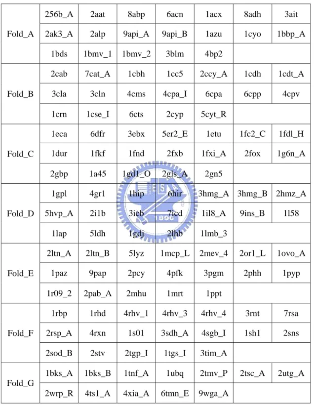
Rost and Sander [1] and referred to as the RS126 set was used to evaluate the accuracy of the prediction. The proteins in the RS126 data set have less than 25% pairwise sequence identity. This set was used to evaluate different methods of relative solvent accessibility prediction, for example, PHDacc [1] and other methods [23], [30], [31]. In this paper, we performed a sevenfold cross-validation test on this set as defined in Table 2.1 [53]. In order to avoid the selection of extremely biased partitions, the RS126 set was divided into subsets of approximately same composition of each type of RSA state. One subset was chosen as the testing set while the rest was merged into the training set. This procedure was repeated seven times to cover whole RS126 data set.

(17)

Table 2.1. The database of non-homologous proteins used for seven-fold cross validation. All proteins have less than 25% pairwise similarity for lengths greater than 80 residues.

256b_A 2aat 8abp 6acn 1acx 8adh 3ait 2ak3_A 2alp 9api_A 9api_B 1azu 1cyo 1bbp_A Fold_A

1bds 1bmv_1 1bmv_2 3blm 4bp2

2cab 7cat_A 1cbh 1cc5 2ccy_A 1cdh 1cdt_A 3cla 3cln 4cms 4cpa_I 6cpa 6cpp 4cpv Fold_B

1crn 1cse_I 6cts 2cyp 5cyt_R

1eca 6dfr 3ebx 5er2_E 1etu 1fc2_C 1fdl_H 1dur 1fkf 1fnd 2fxb 1fxi_A 2fox 1g6n_A Fold_C

2gbp 1a45 1gd1_O 2gls_A 2gn5

1gpl 4gr1 1hip 6hir 3hmg_A 3hmg_B 2hmz_A 5hvp_A 2i1b 3icb 7icd 1il8_A 9ins_B 1l58 Fold_D

1lap 5ldh 1gdj 2lhb 1lmb_3

2ltn_A 2ltn_B 5lyz 1mcp_L 2mev_4 2or1_L 1ovo_A 1paz 9pap 2pcy 4pfk 3pgm 2phh 1pyp Fold_E

1r09_2 2pab_A 2mhu 1mrt 1ppt

1rbp 1rhd 4rhv_1 4rhv_3 4rhv_4 3rnt 7rsa 2rsp_A 4rxn 1s01 3sdh_A 4sgb_I 1sh1 2sns Fold_F

2sod_B 2stv 2tgp_I 1tgs_I 3tim_A

1bks_A 1bks_B 1tnf_A 1ubq 2tmv_P 2tsc_A 2utg_A Fold_G

(18)

2.2 The Definition of Protein Solvent Accessibility

2.2.1 Static Residue Solvent Accessibility

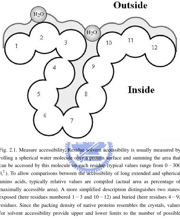
The native structure of globular proteins exists only in the presence of water, and therefore the analysis of their interactions with water is central to the theory of protein structure. The term “accessible surface area” was introduced by Lee and Richards [32] to quantitatively describe the extent to which atoms on the protein surface can form contacts with water. For a particular protein atom it is defined as the area over which the center of a water molecule can be placed while retaining van der Waals contacts with that atom and not penetrating any other atom. The principal goal is to predict the extent to which a residue embedded in a protein structure is accessible to solvent. Solvent accessibility can be described in several ways [32]–[34]. The most detailed fast method compiles solvent accessibility by estimating the volume of a residue embedded in a structure that is exposed to solvent as shown in Fig. 2.1; note: this method was developed by Lee and Richards [32] and later implemented in DSSP [35]. Different residues have a different possible accessible area.

Studies of solvent accessibility in proteins have led to many new insights into protein structure [32]–[37]. Knowledge of solvent accessibility has proved useful for identifying protein function, sequence motifs, and domains, and for formulating hypotheses about antigenic determinants, site-directed mutagenesis, humanization of antibodies, and on the correctness of designed or experimentally determined protein structures. Furthermore, knowledge of solvent accessibility has assisted alignments in regions of remote sequence identity.

(19)

Fig. 2.1. Measure accessibility. Residue solvent accessibility is usually measured by rolling a spherical water molecule over a protein surface and summing the area that can be accessed by this molecule on each residue (typical values range from 0－300 Å2

). To allow comparisons between the accessibility of long extended and spherical amino acids, typically relative values are compiled (actual area as percentage of maximally accessible area). A more simplified description distinguishes two states: exposed (here residues numbered 1－3 and 10－12) and buried (here residues 4－9) residues. Since the packing density of native proteins resembles the crystals, values for solvent accessibility provide upper and lower limits to the number of possible inter-residue contacts.

(20)

2.2.2 Residue Relative Solvent Accessibility

How can the solvent accessibility of a residue embedded in a 3D structure be cast into a simple number? One simple way is to count the number of water molecules in direct contact with the residue, as estimated by the program DSSP for the first hydration shell. For comparison between amino acids of different sizes, the relative solvent accessibility is a useful quantity as defined in Table 2.2.

Amino acid relative solvent accessibility is the degree to which a residue in a protein is accessible to a solvent module. The relative solvent accessibility can be calculated by the formula as follows:

(%) (%) MaxAcc Acc 100 c RelAc = × , (2.1) where Acc is the solvent accessible surface area of the residue observed in the 3D structure, given in Angstrom units, calculated from coordinates by the dictionary of protein secondary structure (DSSP) program [35]. The number of water molecules around a residue can be approximated by Acc/10, and MaxAcc is the maximum value of solvent accessible surface area of each kind of residue for a Gly-X-Gly extended tripeptide conformation.

(21)

Table 2.2. Definition of solvent accessibility states. z Solvent accessibility:

Acc = solvent accessibility of a residue (given in Å2

) calculated from coordinates using DSSP [35]. W≈ Acc/10, approximates the number of water molecules around the residue.

z Relative solvent accessibility:

RelAcc = Acc/MaxAcc, with maximal accessibility (measured in Å2

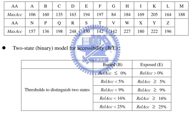
) for the amino acids given by the table following (amino acids in one-letter code; B stands for D or N; Z for E or Q, and X for an undetermined amino acid) [37][38].

AA A B C D E F G H I K L M

MaxAcc 106 160 135 163 194 197 84 184 169 205 164 188

AA N P Q R S T V W X Y Z

MaxAcc 157 136 198 248 130 142 142 227 180 222 196

z Two-state (binary) model for accessibility (B/E) :

Buried (B) Exposed (E)

RelAcc ≤ 0% RelAcc > 0% RelAcc < 5% RelAcc ≥ 5% RelAcc < 9% RelAcc ≥ 9% RelAcc < 16% RelAcc ≥ 16% Thresholds to distinguish two states

RelAcc < 25% RelAcc ≥ 25%

z Three-state (ternary) model for accessibility (B/I/E) :

Buried (B) Intermediate (I) Exposed (E) Thresholds to distinguish three states RelAcc < 9% 9% ≤ RelAcc < 36% RelAcc ≥ 36%

z Measure for evaluation of conservation and accuracy of prediction:

Q2 percentage of conserved, or correctly predicted, residues in two states defined

by thresholds given above.

Q3 percentage of conserved, or correctly predicted, residues in three states

(22)

RelAcc can hence adopt values between 0% and 100%, with 0% corresponding

to a fully buried and 100% to a fully accessible residue, respectively. Different arbitrary threshold values of relative solvent accessibility are chose to define categories: buried and exposed as shown in Fig. 2.2, or ternary categories: buried, intermediate, or exposed. The precise choice of the threshold is not well defined [1].

We used two kind of class definitions: (1) buried (B) and exposed (E); and (2) buried (B), intermediate (I), and exposed (E). For the two-state, B and E definition, we chose various thresholds of the relative solvent accessibility such as 25%, 16%, 9%, 5%, and 0%. For the three-state, B, I, and E, description of relative solvent accessibility, one set of thresholds that we selected is the same as those in Rost and Sander [1]:

Buried (B): RelAcc < 9% Intermediate (I): 9% ≤ RelAcc < 36%

(23)

Fig 2.2. Binary model: thick and dark line is buried residues; thin and light line is exposed residues [39].

(24)

2.3 PSI-BLAST Profiles

It is well known that evolutionary information in the form of multiple alignments and profiles significantly improves the accuracy of, for instance, secondary structure prediction methods [2], [9], [40]–[42]. This is so because the secondary structure of a family is more conserved than the primary amino acid sequence. Similar effects have been reported for the prediction of contact number and relative solvent accessibility. For relative solvent accessibility, a corresponding increase of 5% has been described both with neural networks [40] and Bayesian methods.

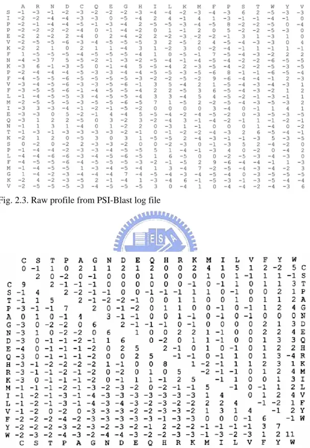
PSI-BLAST [29] generates the profile of a protein in the form of an N×20 position-specific scoring matrix as shown in Fig. 2.3, where N is the length of the sequence. PSI-BLAST is run with default options, -j 3, -h 0.001, and -e 10.0, and the non-redundant protein sequence database (ftp://ncbi.nlm.nih.gov/blast/db) filtered by PFILT [9] to mask out regions of low complexity sequence, the coiled coil regions and transmembrane spans. The BLOSUM62 [43] substitution matrix as shown in Fig. 2.4, is used for PSI-BLAST. These profiles were scaled to the required 0–1 range using the standard logistic function:

, ) ( ) ( x exp 1 1 x f − + = (2.2) where x is the raw profile matrix value.

(25)

Fig. 2.3. Raw profile from PSI-Blast log file

Fig. 2.4. BLOSUM 62 substitution matrix (Lower) and difference matrix (Upper) obtained by subtracting the PAM 160 matrix position by position. These matrices have identical relative entropies (0.70); the expected value of BLOSUM 62 is -0.52; that for PAM 160 is -0.57.

(26)

2.4 K-Nearest Neighbor Algorithm

Nearest neighbor methods are based on learning by analogy. The training samples are described by n-dimensional numeric attributes. Each sample represents a point in an n-dimensional space. In this way, all of the training samples are stored in an n-dimensional pattern space. When given an unknown sample, a k-nearest neighbor classifier searches the pattern space for k training samples that are closest to the unknown sample. The k training samples are the k “nearest neighbors” of the unknown sample. “Closeness” is defined in terms of Euclidean distance, where the Euclidean distance between two points, Xr =(x1,x2,...,xn) and Y =(y1,y2,...,

r ) n y is

∑

= − = n i i i y x Y X d 1 2 ) ( ) , (r r (2.3)

Consider the case of m classes

{

C

_i

}

m_i=1 and a set of N sample patterns

N i i

z

}

₁

{

r

₌

whose classification is a priori known. Let xr denote an arbitrary incoming pattern. The nearest neighbor classification approach classifies xr in the pattern class of its nearest neighbor in the set

{

z

r

i

}

_iN=₁, i.e., if i

N i j x z z xr − r = r − r ≤ ≤ 1min then x∈Cj r

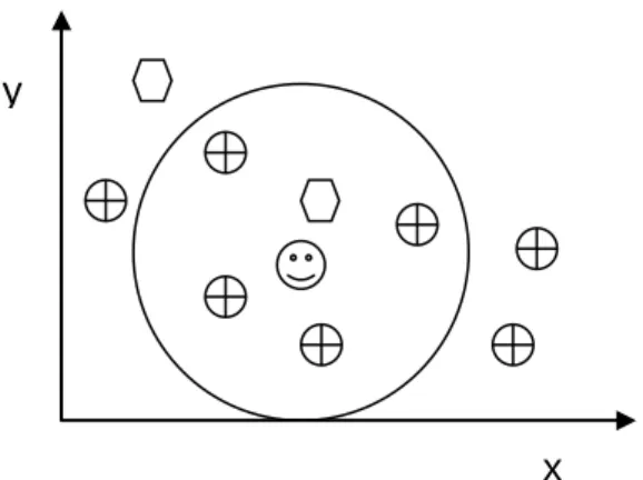
if zrj ∈Cj. This scheme which is basically another type of minimum-distance classification, can be modified by considering the k nearest neighbors to xr and using a majority-rule type classifier. Its advantage is overcoming class noise in the training set. And the example is shown in Fig. 2.5 :

(27)

y

x

Fig. 2.5. Simple 2-D case, each instance is described only by two values (x, y coordinates). The class is either or .

Inside the circle of Fig. 2.5, we can easily see that the class of simple-NN (1-NN) is , and the class of 5-NN is ( is the testing data).

Nearest neighbor classifiers are instance-based or lazy-learners in that they store all of the training samples and do not build a classifier until a new (unlabeled) sample needs to be classified. This contrasts with eager learning methods, such as decision tree induction and back propagation, which construct a generalization model before receiving new samples to classify. Lazy learners can incur expensive computational costs when the number of potential neighbors (i.e., stored training samples) with which to compare a given unlabeled sample is large. Therefore, they require efficient indexing techniques. As expected, lazy learning methods are faster at training than eager methods, but slower at classification since all computation is delayed to that time. Unlike decision tree induction and back propagation, nearest neighbor classifiers assign equal weight to each attribute. This may cause confusion when there are many irrelevant attributes in the data.

(28)

Nearest neighbor classifiers can also be used for prediction, that is, to return a real-valued prediction for a given unknown sample. In this case, the classifier returns the average value of the real-valued labels associated with the k-nearest neighbors of the unknown sample.

(29)

2.5 Quick Radial Basis Function Network

Networks based on radial basis functions have been developed to address some of the problems encountered with training multilayer perceptrons: radial basis functions are usually able to converge and the training is much more rapid. Both are feed-forward networks with similar-looking diagrams and their applications are similar; however, the principles of action of radial basis function networks and the way they are trained are quite different from multilayer perceptrons.

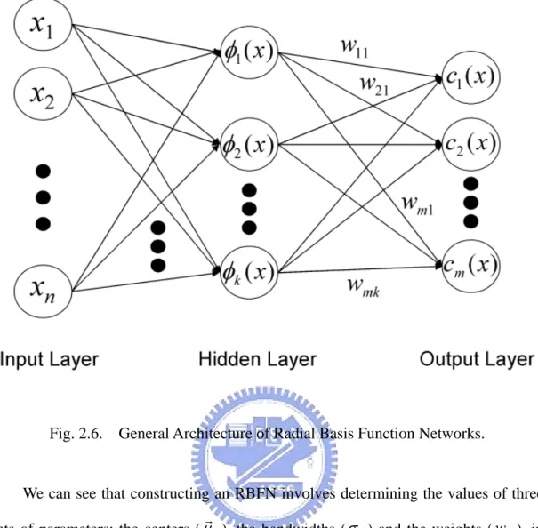
A RBFN (radial basis function network) consists of three layers, namely the input layer, the hidden layer and the output layer. The input layer broadcasts the coordinates of the input vector to each of the nodes in the hidden layer. Each node in the hidden layer then produces an activation based on the associated radial basis function. Finally, each node in the output layer computes a linear combination of the activations of the hidden nodes.

For radial basis function networks, each hidden unit represents the center of a cluster in the data space. Input to a hidden unit in a radial basis function is not the weighted sum of its inputs but a distance measure: a measure of how far the input vector is from the center of the basis function for that hidden unit. Various distance measures are used, but perhaps the most common is the well-known Eculidean distance measure.

The Eculidean distance between them is given by

∑

− = − = i ji i j j x x y D 2 ) (

μ

r r (2.4)

(30)

if xr is an input vector and μrj is the location vector of the basis function for hidden

node j. The hidden node then computes its outputs as a function of the distance between the input vector and its center. For the Gaussian radial basis function the hidden unit output is

hj(Dj2) = 2 j 2 j 2 D

e

− / σ (2.5) whereD is the Euclidean distance between an input vector and the location vector _j for hidden unit j; h is the output of hidden j and_j σj is a measure of the size of the

cluster j (in statistical terms it is called the variance or the square of the standard deviation).

How a RBFN reacts to a given input stimulus is completely determined by the activation functions associated with the hidden nodes and the weights associated with the links between the hidden layer and the output layer. The general mathematical form of the output nodes in an RBFN is as follows:

(

)

∑

= − = k j j ji i rj r x w x c 1 ; ) (r

φ

μ

σ

(2.6) where cr(xr) is the function corresponding to the r-th output unit (class r) and is a linear combination of k radial basis function φ(⋅) with center μrj and bandwidth component σj. Also, wrr is the weight vector of class r and w is the weight rj

corresponding to the r-th class and j-th center. The general architecture of RBFN is shown as follows.

(31)

Fig. 2.6. General Architecture of Radial Basis Function Networks.

We can see that constructing an RBFN involves determining the values of three sets of parameters: the centers (μrj), the bandwidths (σj) and the weights (w ), in rj

order to minimize a suitable cost function.

In QuickRBF package, the centers are randomly selected and bandwidth are fixed and set as 5 for each kernel function for conducting the simplest method. The transformation between the inputs and the corresponding outputs of the hidden units is now fixed. The network can thus be viewed as an equivalent single-layer network with linear output units. Then, the LMSE method is used to determine the weights associated with the links between the hidden layer and the output layer.

(32)

[

φ

1(xr),

φ

2(xr) ,K,

φ

k(xr )

]

T

=

h (2.7) where k is the number of centers, φ1(xr) is the output value of first kernel function

with input xr. Then, the discriminant function cr(xr) of class r can be expressed by

the following:

cr(xr)=wrrTh , r =1,2,K,m (2.8) where m is the number of class, and wr is the weight vector of class r. We can show r

r

wr as:

[

w x w x , w x

]

wr =r r1(r), r2(r) K, rk(r) T (2.9)

After calculating the discriminant function value of each class, we choose the class with the biggest discriminant function value as the classification result. We will discuss how to get the weight vectors by using least mean square error method in the following.

For a classification problem with m classes, let Vrr designate the r-th column

vector of an m × m identity matrix and W be an k × m matrix of weights:

W =

[

wr1, wr2,..., wrm

]

(2.10)

Then the objective function to be minimized

J PE V m r r T r r

∑

= ⎭⎬ ⎫ ⎩ ⎨ ⎧ ₋ = 1 2 ) (W W h r (2.11) where P and r Er{ ⋅} are the a priori probability and the expected value of class r,

respectively.

(33)

( ) 2

{ }

2

{ }

[ ] 1 1 0 h W hh W = − = ∇

∑

= = T r m r r r m r T r r wJ P E PE Vr (2.12)

where [0] is a k × m null matrix. Let K denote the class-conditional matrix of the r

second-order moments of h, i.e.

{ }

T

r

r E hh

K = (2.13) If K denotes the matrix of the second-order moments under the mixture distribution,

we have

∑

= = m 1 r r r P K K (2.14) Then Eq. (2.12) becomes

KW=M (2.15) where PE

{ }

V m r T r r r

∑

= = 1 r h M (2.16) If K is nonsingular, the optimal W can be calculated by

W* =K-1M

(2.17)

However, there is a critical drawback of this method. That is, K may be singular

and this will crash the whole procedure. By observing the matrix hh , we are aware T

of that the matrix hh is symmetric positive semi-definite (PSD) matrix with rank T

equal to 1. Since K is the summation of hh for each training instance, K is also a T

PSD matrix with rank smaller than n. However, PSD matrix may be a singular matrix, so we should add the regularization term to make sure the matrix will be invertible. In the regularization theory, it consists in replacing the objective function as follows:

rT r m r m r r T r rE V w w P J

∑

r

∑

r r = = + ⎭ ⎬ ⎫ ⎩ ⎨ ⎧ ₋ = 1 1 2 ) (W W h

λ

(2.18)

(34)

where λ is the regularization parameter. Then the Eq. (2.15) becomes

(

K+λI

)

W=M (2.19)

If we set λ >0,

(

K+λI

)

will be a positive definite (PD) matrix and therefore is nonsingular.The optimal W* can be calculated by

W* =

(

K+λI

)

-1M (2.20)

However, the PD matrix has many good properties, and one of them is a special and efficient triangular decomposition, Cholesky decomposition. By using Cholesky decomposition, we can decompose the

(

K+λI

)

matrix as follows:

(

)

T

LL I

K+λ = (2.21) where L is a lower triangular matrix. Then, the Eq. (2.19) becomes

(

LLT

)

W=M (2.22) Actually, the linear system can be solved efficiently by using back-substitution twice. Finally, we can get the optimal W for class r from r* W , and then the *

optimal discriminant function cr(xr) for class r is derived. By using the

(35)

Chapter 3. Protein Relative Solvent Accessibility Prediction

3.1 Fuzzy K-Nearest Neighbor Approach

The nearest neighbor algorithm is a simple classification algorithm; a query data

is classified according to the classification of the nearest neighbor from a database of known classifications. A natural generalization of the nearest neighbor algorithm is the so-called k-nearest neighbor algorithm, where the k-nearest samples are selected and the query data is assigned the class most frequently represented among them. A further extension is to weight the k-nearest samples with a certain power of the distance from the query data. Also, instead of assigning a definite class to the query data, one can calculate the fuzzy membership (see below), which can be used to reflect the confidence level of each nearest neighbor in its prediction. The algorithm incorporating these generalizations is called the fuzzy k-nearest neighbor algorithm [18].

Despite its simplicity, nearest neighbor methods can give competitive performance compared to many other methods. The nearest neighbor methods have been used to predict protein secondary structure [26]–[28] and classify biological and medical data. Also it has been reported that performances of classification were improved by using fuzzy k-nearest neighbor algorithms [44]–[49]. However the

k-nearest neighbor method has few been used to predict protein solvent accessibility.

As with Hua and Sun’s work [50], the present analysis used the classical local

(36)

with n rows and 20 columns can be defined for single sequence with n residues. Each residue is represented using 20 components in a vector, based on the PSSM. Then, each input vector has 20×w components, where w is a sliding window size.

They constructed a window of size 15 centered on a target residue [9], [23], [24], and use the profile that falls within this window, a 15×20 matrix, as a feature vector. Then, the distance between two feature vectors A and B is defined as

=

∑

− j i B ij A ij i AB W P P D , ) ( ) ( , (3.1) where P_ij( A)( i = 1, 2,…, 15; j = 1, 2,…, 20) is a component of the feature vector A,

and W is a weight parameter. Since it is expected that the profile elements for _i residues nearer to the target residue to be more important in determining the local environment of the target residue, weights W are set to i W_i =(8− 8−i)2.

In their work, they applied the fuzzy k-nearest neighbor method to the solvent accessibility prediction. In the fuzzy k-nearest neighbor method, the fuzzy class membership )u_i(x to the class i is assigned to the query data x according to the following equation: , ) ( ) ( ) /( ) /( ) (

∑

= − − − − = = _k 1 j 1 m 2 j 1 m 2 j j k 1 j i i D D x u x u i = 1, 2,…, c, (3.2)

where m is a fuzzy strength parameter, which determines how heavily the distance is weighted when calculating each neighbor’s contribution to the membership value, k is the number of nearest neighbors, and c is the number of classes. Also, D is the _j distance between the feature vector of the query data x and the feature vector of its

(37)

the i th class, which is 1 if x belongs to the i th class, and 0 otherwise. The ( j) advantage of the fuzzy k-nearest neighbor algorithm over the standard k-nearest neighbor method is quite clear. Modulating the ith neighbor’s fuzzy class membership

) (x

u_i through its percentile distance to the query residue can be considered as the estimate of the probability that the query data belongs to class i, and provides us with more information than a definite prediction of the class for the query data. Moreover, the reference samples which are closer to the query data are given more weight, and an optimal value of m can be chosen along with that for k, in contrast to the standard

k-nearest neighbor method with a fixed value of 2/(m－1) = 0. In fact, the optimal

value of k and m are found from the leave-one-out cross-validation procedure, and the resulting value for 2/(m－1) is indeed nonzero.

We adopt the optimal values of m and k in [31], which are (m, k) = (1.33, 65) for the 3-state prediction (for both 9% and 36% thresholds) and (m, k) = (1.50, 40), (1.25, 75), (1.29, 65) and (1.33, 65) for the 2-state predictions (for 0, 5, 16, and 25% thresholds, respectively). Moreover, we use (m, k) = (1.27, 70) for the 9% threshold, whose prediction accuracy is slightly higher than other (m, k) values.

3.2 Modified Fuzzy K-Nearest Neighbor Approach

In Sec. 3.1 above, we can see u_i(x( j)) is defined as the membership value of

) ( j

x to the i th class, which is 1 if _{x belongs to the i th class, and 0 otherwise.}( j)

Here, we modify the definition of u_i(x( j)) in Eq.(3.2). It is expected that a neighbor residue close to the threshold RelAcc chosen is not as decisive in determining query

(38)

values as a neighbor residue far from the residue’s RelAcc state. For two-state model for accessibility, as shown in Table 2.2, we have to choose a threshold to distinguish the two states (Buried and Exposed). If we choose a value Th (must between 0 and 1) as our threshold, the residues where Relacc values range from 0 to Th will be classified to the buried state, and others (from Th to 100%) will be classified to the exposed state. So the two boundaries of buried class are 0 and Th, and the two of buried one are Th and 1. The range lies in [0, Th] for the buried state and [Th, 1] for the exposed state.

It is known that 0 is the minimum for RelAcc value, and 1, 100%, is the maximum. That means 0 is the most buried point and 100% is the most exposed one.

For each residue of a protein sequence, we can calculate a “buried distance, D_B” which represents the “distance” from present residue to 0 and a “exposed distance,

E

D ” which represents the “distance” from present residue to 1. If the RelAcc value of a residue is smaller than Th, then we calculate its D_B and D_E values by the following equations: , Th RelAcc DB = Th RelAcc Th 1 DE = + − .

In contrast, if the RelAcc value is larger than Th, we calculate the D_B and D_E values by the equation shown below:

, Th 1 Th RelAcc 1 DB − − + = Th 1 RelAcc 1 DE − − = .

(39)

residue should be small. That is, D_B is inversely proportional to the “buried degree.” Similarly, D_E value is also inversely proportional to the “exposed degree.” With this concept in mind, we can use D_B and D_E to calculate membership values u_i(x( j)):

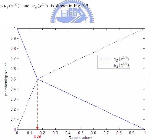
, / / / ) ( ) ( ( ) ( ) B E E j E j 1 D 1 D 1 D 1 x u x u + = = . / / / ) ( ) ( ( ) ( ) B E B j B j 2 D 1 D 1 D 1 x u x u + = = Obviously, if we let ( ( ))= ( (j))=0.5 E j B x u x

u in both conditions (buried an exposed) to calculate RelAcc value, then we will obtain that RelAcc = Th. That means the membership values of both classes at the threshod Th are 50%. The membership functions are shown in Fig. 3.1. The flowchart to calculate 2-state membership values ( ( j))

E x

u and ( ( j))

B x

u is shown in Fig. 3.2.

Fig. 3.1. The 2-state membership functions ( ( j))

E x

u and ( ( j))

B x

(40)

Fig. 3.2. The flowchart to calculate 2-state membership values u₁(x(j)) and ) ( ( ) 2 j x u .

(41)

the boundaries are 0 and 9% for the buried state, 9% and 36% for the intermediate state, 36% and 100% for the exposed state, so the center value of the intermediate class, . . , 2 36 0 09 0 +

is 0.225. u_B(x( j)) is set to zero when the RelAcc value of a residue is greater than 0.225, so we can calculate u_I(x( j)) and u_E(x( j)) by two-class method given above. In the same manner, we set the ( ( j))

E x

u to zero when RelAcc value is smaller than 0.225, and we can calculate u_I(x( j)) and

) ( ( j)

B x

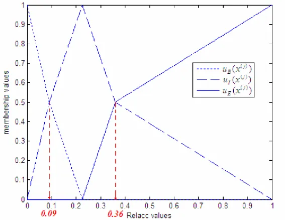
u as above. The three-state membership functions are shown in Fig. 3.3. The flowchart to calculate 3-state membership values is shown in Fig. 3.4.

Fig. 3.3. The 3-state membership functions u_E(x( j)), )u_I(x( j) , and u_B(x( j)) with

Ths = 9% and 36%.

Therefore, in this setting of membership functions, the values of ( ( j))

i x

(42)

∑

= = c i j i x u 1 ) ( 1 )

( . After this modification, we continue to calculate all the u_i(x) by Eq. (3.2) by the method shown in Sec.3.1, and the maximal ui(x) class is assumed to be

the target class of the residue x.

Fig. 3.4. The flowchart to calculate 3-state membership values u_E(x( j)),u_I(x( j)), and )u_B(x( j) .

(43)

3.3 QuickRBF Approach

A QuickRBF structure used for solvent accessibility prediction system are shown in Fig. 3.5. The QuickRBF classifier classifies each residue of each sequence into the three relative solvent accessibility states, E, I, or B, by using the values of matrices of PSI-BLAST profile as the inputs. The outputs represent the tendency that the residue belongs to that state. The one-against-rest strategy was used for the multiclass classification, so each residue was classified into the state with the largest output value for a QuickRBF approach.

(44)

Fig. 3.5. Architecture of QuickRBF method. The system includes two parts: the PSI-BLAST profile, and the classifier. The profile is transformed into a number of 21*17 dimension vectors using the slide-window method. These vectors are input into the QuickRBF classifier. The outputs of the QuickRBF classifier are a number of 3D vectors representing the tendency that the residue belongs to that state. The one-against-rest strategy was used to classify each residue into the state with the largest value.

PSI-BLAST Profile

Coding : transform the 17*20 matrix into a 17*21 dimension vector

QuickRBF Classifier Data Normalization

Classifier

(45)

3.4 Fusion Method

3.4.1 Linear Combination Fusion 1

We have proposed modified fuzzy k-NN approach and QuickRBF approach, both based on the PSSM profiles, to predict the protein relative solvent accessibility. We have found the differences of predictive results between the two approaches are somewhat distinct. This motivates us to design a fusion scheme combining the results of both approaches in order to raise the overall accuracy.

After observing the output values of modified fuzzy k-NN and QuickRBF, we found their dynamic ranges are different. In modified fuzzy k-NN approach shown in Sec. 3.2, the membership values u_i(x( j)) of all the two or three classes calculated range between 0 to 1, but the outputs of the QuickRBF approach do not vary in this range. We need to normalize them first before we can make the fusion. Here, we calculated the mean of each class in three-state prediction result for each method, respectively. For each method, these three values (mE,mI, and m ) were used as the B

“normalization factor.” We divided all the prediction results of each class by its mean to get normalized output. At last, we combined by adding the normalized output of both methods, and the final output class of each residue is assigned to the one with the largest output value. This normalization procedure is shown in Fig. 3.6. The normalization was done similarly in the two-state case.

(46)

Fig. 3.6. The normalization procedure in Linear Combination Fusion 1.

Referring to Table 3.1, each residue of the present sequence has three target labels denoted as E, I and B. The respective results of each label are the linear

combination of results of the normalized QuickRBF and modified fuzzy k-NN. Then the final output class of each residue is assigned to the one with the largest output value. Namely, it applies

P(x( )) argmax fl(x(j)) (l {E,I,B}, j 1, 2,..., m)

l j

l = ∈ = (3.3)

where fl are the linearly combined values shown below:

) ( ) ( ) ( ) ( ) ( ) ( ) ( ) ( ) ( 2 1 2 1 2 1 j B j B j B f j I j I j I f j E j E j E f f B f I f E + = = + = = + = = (3.4)

(47)

Table 3.1. Fusion method : Linear combination.

3.4.2 Linear Combination Fusion 2

We have also developed a different normalization method in this section. We obtained the absolute values of a residue in QuickRBF output data, and summed them up as the “normalization factor.” Then, we divided all the three prediction values E, I, and B of the residue by the normalization factor to obtain their respective normalized outputs. After the normalization, we combined the normalized output by adding the modified fuzzy k-NN and QuickRBF in the same method shown in Sec. 3.4.1. This normalization procedure is shown in Fig. 3.7.

(48)

Fig. 3.7. The normalization procedure in Linear Combination Fusion 2.

3.4.3 Reliability Index

The prediction reliability index (RI) was used to access the effectiveness of the approaches for the prediction of the secondary structure of a new sequence. The RI offers an excellent tool for focusing on key regions having high prediction accuracy. Hence, we used reliability index in protein relative solvent accessibility prediction. There are different definitions of the RI. Here we used a definition similar to that proposed by Rost and Sander: RI = maximal_output(I)－Second_largest_output(I) [51]. If the value of RI > 0.9, then set RI = 0.9, so the value of RI is between 0 and 0.9. The prediction accuracy of residues with higher RI values is much better than those with lower RI values. Therefore, the definition of RI reflects the prediction reliability.

(49)

QuickRBF (after normalization shown in 3.4.2), we developed a new classifier design using RI. In this scheme, the classifier with a maximum RI is chosen as the arbiter classifier for the decision of the class. The final class is chosen to the largest output class of this arbiter classifier. For example, if the E/I/B output of the decision function of QuickRBF: E/I/B, modified fuzzy k-NN: E/I/B are 0.1/0.2/0.7 and 0.3/0.2/0.5, their RI’s are 0.5, 0.7－0.2, and 0.2, 0.5－0.3, respectively. Therefore, the classifier with highest RI, here QuickRBF, is chosen as the arbiter. In this example, the query residue is assigned to be buried since it is the largest class value of the QuickRBF classifier.

(50)

Chapter 4. Experiment and Simulation Results

4.1 Datasets

The set 126 nonhomologous globular protein chains used in the experiment of

Rost and Sander [1], referred to as the RS126 set, was utilized to evaluate the accuracy of the classifiers. The RS126 dataset contains 23606 residues. Fuzzy

K-Nearest Neighbor approaches and QuickRBF approaches were implemented with

multiple sequence alignments, and tested on the dataset using a seven-fold cross validation technique to estimate the prediction accuracy. With seven-fold cross validation, approximately six-seventh of the RS126 dataset was selected for training and, after training, the left one-seventh of the dataset was used for testing. In order to avoid the selection of extremely biased partitions, the RS126 set was divided, by [53] previously, into seven subsets with each subset having similar size as shown in Table 2.1.

(51)

4.2 Results

4.2.1 Results of Fuzzy K-NN and Modified Fuzzy K-NN Classifiers

Fuzzy k-nearest neighbor approaches are applied on three-state, E, I, and B, and two-state, E and B, relative solvent accessibility predictions. For both classifiers, each residue of sequences is coded as a 20-dimensional vector, which the 20 elements of the vector are the corresponding elements in PSI-BLAST matrix. The window length is 15 and the dimension of the feature vector is 20×15.

The results and the comparison of the fuzzy k-nearest neighbor approach and modified fuzzy k-nearest neighbor approach on RS126 data set are listed in Table 4.1.

On the RS126 data set processed by ourselves, fuzzy k-nearest neighbor approach [31]

led to the overall prediction accuracy 58.14% for the three-state prediction with respect to thresholds: 9% and 36%; and 87.93%, 79.18%, 77.59%, 75.35%, 73.49% for the two-state prediction with the thresholds of 0%, 5%, 9%, 16%, and 25%, repectively.

Modified fuzzy k-nearest neighbor approach gave the overall prediction accuracy 58.57% for the three-state prediction with respect to the following two thresholds chosen: 9% and 36%; and 87.93%, 79.84%, 77.76%, 76.34%, 75.26% for the two-state prediction with the chosen thresholds of 0%, 5%, 9%, 16%, and 25%, respectively.

(52)

Table 4.1. RSA classification accuracy of ours and previous fuzzy k-nearest neighbor methods on the RS126 data set with PSI-BLAST pssm profiles.

Fuzzy k-NN classifiers [31] Accuracy: % thresholds dataset 3-state (9% ; 36%) 2-state (0%) 2-state (5%) 2-state (9%) 2-state (16%) 2-state (25%) Fold_A 58.33 86.37 78.63 76.10 75.00 73.97 Fold_B 58.22 88.93 79.84 78.76 76.14 73.17 Fold_C 61.23 87.93 80.11 79.22 77.74 76.18 Fold_D 57.01 88.38 78.28 77.30 74.26 72.65 Fold_E 58.52 88.75 79.90 79.21 76.21 73.15 Fold_F 55.90 88.99 79.54 77.19 73.22 71.20 Fold_G 57.30 86.38 78.09 75.39 74.52 73.66 Average 58.14 87.93 79.18 77.59 75.35 73.49

Ours modified fuzzy k-NN classifiers

Accuracy: % thresholds dataset 3-state (9% ; 36%) 2-state (0%) 2-state (5%) 2-state (9%) 2-state (16%) 2-state (25%) Fold_A 59.14 86.37 77.90 77.50 77.27 76.61 Fold_B 59.00 88.93 81.35 78.52 77.03 75.49 Fold_C 60.39 87.93 80.92 78.52 77.71 77.08 Fold_D 57.99 88.38 80.33 77.30 75.40 74.81 Fold_E 59.84 88.75 81.54 77.99 76.21 74.99 Fold_F 56.95 88.99 79.54 77.59 74.31 72.54 Fold_G 55.80 86.38 77.26 76.77 75.72 74.22 Average 58.57 87.93 79.84 77.76 76.34 75.26

(53)

4.2.2 Results of QuickRBF approach and the Fusion Methods

For QuickRBF approach, each residue is coded as a 21-dimensional vector, where the first 20 elements of the vector are the corresponding elements in PSI-BLAST matrix and the last element was added in order to allow a window to extend over the N- and the C-terminus. The window length is 17 and the dimension of the feature vector is 21×17. The number of the centers randomly selected from the training data set is 2000 and the bandwidth is five for each kernel function. The architecture of QuickRBF in the three-state prediction is shown in Fig. 3.5, Sec. 3.3.

QuickRBF approach produced the overall prediction accuracy 60.36% for the three-state prediction with respect to thresholds: 9% and 36%; and 87.76%, 81.15%, 79.06%, 77.64%, 76.17% for the two-state prediction with the thresholds of 0%, 5%, 9%, 16%, and 25%, respectively.

Linear Combination Fusion 1, column mean normalization and then adding, gave the overall prediction accuracy 61.30% for the three-state prediction with respect to thresholds: 9% and 36%; and 71.38%, 75.35%, 77.18%, 77.90%, 76.60% for the two-state prediction with the thresholds of 0%, 5%, 9%, 16%, and 25%, respectively. Obviously, the two-state prediction accuracies of thresholds 0%, 5%, and 9% are lower than those by QuickRBF approach.

Linear Combination Fusion 2, row-wise normalization and then adding, led to the overall prediction accuracy 61.06% for the three-state prediction with respect to thresholds: 9% and 36%; and 87.97%, 81.28%, 79.77%, 78.23%, 76.96% for the

(54)

Reliability Index Fusion, maximal relative index, gave the overall prediction accuracy 61.09% for the three-state prediction with respect to thresholds: 9% and 36%; and 87.97%, 81.24%, 79.73%, 78.16%, 77.01% for the two-state prediction with the thresholds of 0%, 5%, 9%, 16%, and 25%, respectively. The prediction accuracies of QuickRBF and the fusion methods on RS126 data set are listed in Table 4.2.

Table 4.2. RSA classification accuracies by QuickRBF and the fusion methods.

QuickRBF accuracy: % thresholds dataset 3-state (9%＆36%) 2-state (0%) 2-state (5%) 2-state (9%) 2-state (16%) 2-state (25%) Fold_A 60.71 86.51 79.40 78.30 77.64 76.38 Fold_B 60.67 89.15 81.35 79.60 78.06 76.38 Fold_C 61.81 87.59 80.92 80.25 78.90 77.17 Fold_D 59.16 88.01 81.29 78.46 76.96 75.51 Fold_E 60.85 88.51 82.76 80.53 78.65 76.07 Fold_F 58.90 88.74 81.13 78.02 76.00 74.27 Fold_G 60.23 85.85 78.35 78.35 77.00 77.26 Average 60.36 87.76 81.15 79.06 77.64 76.17

Linear Combination Fusion 1

of accuracy: % thresholds dataset 3-state (9%＆36%) 2-state (0%) 2-state (5%) 2-state (9%) 2-state (16%) 2-state (25%) Fold_A 62.14 72.08 75.91 77.39 78.46 77.15 Fold_B 61.16 71.15 76.03 77.25 78.22 77.11 Fold_C 63.97 72.89 76.73 78.72 79.27 77.83 Fold_D 59.91 70.47 74.00 75.22 76.91 75.95 Fold_E 62.21 70.74 75.72 78.13 78.61 76.77 Fold_F 59.22 71.02 75.57 76.25 75.60 75.10 Fold_G 59.89 70.99 76.59 77.56 77.79 75.72 Average 61.30 71.38 75.75 77.18 77.90 76.60

(55)

Linear Combination Fusion 2 accuracy: % thresholds dataset 3-state (9%＆36%) 2-state (0%) 2-state (5%) 2-state (9%) 2-state (16%) 2-state (25%) Fold_A 61.48 86.53 80.12 78.95 78.51 77.88 Fold_B 61.13 89.45 81.48 80.59 78.60 77.11 Fold_C 63.66 87.73 82.48 81.06 79.22 78.44 Fold_D 60.09 88.30 81.03 79.01 77.71 76.16 Fold_E 61.83 88.61 83.32 80.91 78.75 76.63 Fold_F 59.18 89.07 81.20 79.00 76.54 75.17 Fold_G 59.48 86.27 79.59 78.91 77.90 76.74 Average 61.06 87.97 81.28 79.77 78.23 76.96

Reliability Index Method

accuracy: % thresholds dataset 3-state (9%＆36%) 2-state (0%) 2-state (5%) 2-state (9%) 2-state (16%) 2-state (25%) Fold_A 61.58 86.53 80.17 78.95 78.27 78.04 Fold_B 60.95 89.42 81.40 80.54 78.68 77.06 Fold_C 63.22 87.64 82.45 80.95 79.10 78.55 Fold_D 60.15 88.32 80.88 78.88 77.66 76.28 Fold_E 62.07 88.58 83.14 80.88 78.75 76.73 Fold_F 59.58 89.07 81.05 79.11 76.40 75.03 Fold_G 59.63 86.27 79.85 78.95 77.94 76.70 Average 61.09 87.96 81.24 79.73 78.16 77.01

(56)

Table 4.3. Comparison of performance of the six approaches in RSA prediction on the RS126 data set with PSSMs generated by PSI-BLAST.

Comparison of six methods

accuracy: % thresholds method 3-state (9%＆36%) 2-state (0%) 2-state (5%) 2-state (9%) 2-state (16%) 2-state (25%) Fuzzy k-NN 58.14 87.93 79.18 77.59 75.35 73.49 Modified fuzzy k-NN 58.57 87.93 79.84 77.76 76.34 75.26 QuickRBF 60.36 87.76 81.15 79.06 77.64 76.17

Linear Combination Fusion 1 61.30 71.38 75.75 77.18 77.90 76.60

Linear Combination Fusion 2 61.06 87.97 81.28 79.77 78.23 76.96

(57)

4.3 Matthew’s Correlation Coefficients of Modified Fuzzy K-NN Approach

Another measure used to evaluate the performance of prediction methods is the Matthew’s Correlation Coefficient (MCC). It can be calculated from an accuracy table

A by the following equations:

ij

A = number of residues predicted to be in type j and observed to be in type i,

) )( )( )( ( _i _i _i _i _i _i _i _i i i i i i o n u n o p u p o u n p MCC + + + + − = , i p = A , _ii i n = , 3 3

∑∑

≠i ≠ j k i jk A i o = , 3

∑

≠i j ji A i u = , 3

∑

≠i j ij A for i = E, I, B.

Also, pi , ni , oi and ui are the number of true positives, true negatives, false positives

and false negatives for class i, respectively. The MCCs have the same value for the two classes in the case of the two-state prediction, i.e. MCCE = MCCB.

First, the accuracy tables A of modified fuzzy k-NN approach on each fold and the RS126 data set is shown in Table 4.3. Then, the MCCs of five methods on the RS126 data set is shown in Table 4.4. In a similar trend as Table 4.2, MCC’s of Linear Combination Fusion 2 usually perform well, although not always the best, in comparison to other approaches.

(58)

Table 4.4. The accuracy tables A of modified fuzzy k-NN on each fold and RS126. 3-state (9%; 36%) AEE AII ABB AEI AEB AIE AIB ABE ABI Fold_A 1073 525 931 384 67 432 263 253 348 Fold_B 1068 419 699 313 60 442 229 186 289 Fold_C 847 467 778 356 66 314 245 134 257 Fold_D 1003 491 741 336 97 439 266 182 299 Fold_E 737 376 605 288 56 276 177 135 221 Fold_F 755 320 503 229 52 356 159 168 229 Fold_G 724 435 827 375 172 367 402 167 382 RS126 6207 3033 5084 2281 570 2626 1741 1225 2025 2-state (25%) AEE ABB AEB ABE Fold_A 1515 1761 468 532 Fold_B 1456 1341 388 520 Fold_C 1209 1461 420 374 Fold_D 1389 1494 453 518 Fold_E 1021 1132 379 339 Fold_F 1031 979 335 426 Fold_G 880 1098 354 333 RS126 8501 9266 2797 3042 2-state (16%) AEE ABB AEB ABE Fold_A 1942 1362 431 541 Fold_B 1832 1022 399 452 Fold_C 1563 1129 414 358 Fold_D 1790 1116 471 477 Fold_E 1327 861 352 331 Fold_F 1330 729 300 412 Fold_G 1147 871 320 327 RS126 10931 7090 2687 2898

(59)

Table 4.4. (continued) 2-state (9%) AEE ABB AEB ABE Fold_A 2294 1014 450 518 Fold_B 2151 758 380 416 Fold_C 1877 844 418 325 Fold_D 2164 811 468 411 Fold_E 1580 659 330 302 Fold_F 1595 554 276 346 Fold_G 1375 675 313 302 RS126 13036 5315 2635 2620 2-state (5%) AEE ABB AEB ABE Fold_A 2588 774 440 474 Fold_B 2369 589 400 347 Fold_C 2104 671 398 291 Fold_D 2412 605 454 383 Fold_E 1771 523 327 250 Fold_F 1782 422 266 301 Fold_G 1558 523 315 269 RS126 14584 4107 2600 2315 2-state (0%) AEE ABB AEB ABE Fold_A 3612 81 40 543 Fold_B 3263 32 34 376 Fold_C 2961 85 49 369 Fold_D 3355 51 23 425 Fold_E 2499 49 37 286 Fold_F 2425 41 26 279 Fold_G 2261 41 17 346 RS126 20376 380 226 2624

(60)

Table 4.5. Matthew’s Correlation Coefficients of the five approaches on RS126. 3-state (9%; 36%) MCC method MCCE MCCI MCCB Fuzzy k-NN 0.439 0.133 0.499 Modified fuzzy k-NN 0.432 0.163 0.485 QuickRBF 0.478 0.138 0.529

Linear Combination Fusion 1 0.491 0.176 0.533 Linear Combination Fusion 2 0.487 0.171 0.533

2-state (25%) MCC method MCCE = MCCB Fuzzy k-NN 0.492 Modified fuzzy k-NN 0.505 QuickRBF 0.530

Linear Combination Fusion 1 0.539

(61)

Table 4.5. (continued) 2-state (9%) MCC method MCCE = MCCB Fuzzy k-NN 0.470 Modified fuzzy k-NN 0.501 QuickRBF 0.510

After comparing the prediction results of three fusion methods, we can find that the two-state prediction accuracies of Linear Combination Fusion 1 are lower than

(62)

those by the other two fusion methods with thresholds 0%, 5%, and 9%. In our opinion, this maybe due to the normalization step used in Linear Combination Fusion 1. If the chosen threshold Th is close to zero in two-state modified fuzzy k-NN prediction, then the uB(x( j)) values for most residues will be very low. And hence,

B

m will be close to zero, as shown in Fig. 3.6. After dividing all uB(x( j)) values by

B

m , the new uB(x( j)) values will become very large, and this will cause the faulty classification after the fusion.

4.4 Comparison with other Approaches

For RSA prediction on the RS126 data set, the performance comparison of our approach to other methods is shown in Table 4.6. The Linear Common Fusion 2 is the best in most cases. It is reported 61.1% for the three-state prediction with respect to thresholds of 9% and 36%; 88.0%, 81.3%, 79.8%, 78.2%, and 77.0% for the two-state predictions with the thresholds of 0%, 5%, 9%, 16%, and 25%, respectively.

Sim et al. has led to slightly better prediction accuracies than other methods by fuzzy k-nearest neighbor method using PSI-BLAST profiles on the RS126 data set produced by them. In [31], they reported 63.8% for the three-state prediction with respect to thresholds of 9% and 36%; 87.2%, 82.2%, 79.0%, and 78.3% for the two-state predictions with the thresholds of 0%, 5%, 16%, and 25%, respectively. Using the same method and best parameter settings on our produced RS126 data set, we just obtained 58.1% for the three-state prediction; 87.9%, 79.2%, 75.4%, and

(63)

respectively.

PHDacc [1] used a neural network method using evolutionary profiles of amino acid substitutions derived from multiple sequence alignments, and reported 57.5% for the three-state prediction with respect to thresholds of 9% and 36%; 86.0%, 74.6%, and 75.0% for the two-state predictions with the thresholds of 0%, 9%, and 16%, respectively.

SVMpsi [23] was based on a support vector machine using the position-specific scoring matrix generated from PSI-BLAST, and reported 59.6% accuracy for the three-state prediction with respect to thresholds of 9% and 36%; 86.2%, 79.8%, 77.8%, and 76.8% for the two-state predictions with the thresholds of 0%, 5%, 16%, and 25%, respectively.

Two-Stage SVMpsi [30] used a Two-Stage SVMpsi approach using the position-specific scoring matrix generated from PSI-BLAST. It is reported 90.2%, 83.5%, 81.3%, and 79.4% for the two-state predictions with the thresholds of 0%, 5%, 9%, and 16%, respectively. These prediction accuracies are obtained from their published results.

模糊K-最近相鄰點分類法於蛋白質可溶性預測

國 立 交 通 大 學

電 機 與 控 制 工 程 研 究 所

碩 士 論 文

模糊

K-最近相鄰點分類法於蛋白質可溶性預測

Fuzzy K-Nearest Neighbor Classifier to Predict Protein

Solvent Accessibility

學 生： 施 逸 祥

指 導 教 授： 張 志 永

模糊

K-最近相鄰點分類法於蛋白質可溶性預測

Fuzzy K-Nearest Neighbor Classifier to Predict Protein

Solvent Accessibility

學 生 : 施逸祥 Student : Yi-Xiang Shi

指導教授 : 張志永 Advisor : Jyh-Yeong Chang

國立交通大學

電機與控制工程學系

碩士論文

A Thesis

Submitted to Department of Electrical and Control Engineering

College of Electrical Engineering and Computer Science

National Chiao Tung University

in Partial Fulfillment of the Requirements

for the Degree of Master in

Electrical and Control Engineering

July 2007

Hsinchu, Taiwan, Republic of China

模糊 K-最近相鄰點分類法於蛋白質可溶性預測

摘要

Fuzzy K-Nearest Neighbor Classifier to Predict Protein

Solvent Accessibility

Abstract

Acknowledgement

Contents

List of Figures

List of Tables

Chapter 1. Introduction

Chapter 2. The Data Set Used and Previous Algorithms

∑

{

C

}

z

}

{

r

{

z

r

}

∑

μ

e

(

)

∑

φ

μ

σ

[

φ

φ

φ

]

[

]

[

]

∑

{ }

{ }

∑

∑

{ }

∑

{ }

∑

∑

∑

國立交通大學

電機與控制工程研究所

碩士論文

學生：施逸祥

指導教授：張志永

學生 : 施逸祥 Student : Yi-Xiang Shi