基於傳遞函數比與非線性H∞濾波器之穩健適應性語音純化波束形成器

國 立 交 通 大 學

電控工程研究所

博 士 論 文

基於傳遞函數比與非線性

H

_∞

濾波器之穩

健適應性語音純化波束形成器

Robust Adaptive Beamformer for Speech

Enhancement based on the Transfer Function Ratio

and Nonlinear H

_∞

Filter

研究生：楊佳興

指導教授：胡竹生

中華民國九十九年十二月

基於傳遞函數比與非線性

H

∞

濾波器之穩健適應性

語音純化波束形成器

Robust Adaptive Beamformer for Speech Enhancement

based on the Transfer Function Ratio and

Nonlinear H

∞

Filter

研 究 生：楊 佳 興 Student：Chia-Hsin Yang

指導教授：胡 竹 生

Advisor：Jwu-Sheng Hu

國立交通大學

電控工程研究所

博 士 論 文

A Dissertation

Submitted to Institute of Electrical Control Engineering

College of Electrical and Computer Engineering

National Chiao Tung University

in partial Fulfillment of the Requirements

for the Degree of

Doctor of Philosophy

in

Institute of Electrical Control Engineering

Dec. 2010

基於傳遞函數比與非線性

H

_∞

濾波器之

穩健適應性語音純化波束形成器

研究生：楊佳興

指導教授：胡竹生 教授

國立交通大學電控工程研究所博士班

摘要

在過去三十年中，利用麥克風陣列純化語音的技巧已受到許多研究者的專 注。在許多現實環境中，目標語音訊號通常受穩態雜訊與多個非穩態雜訊所干 擾。本論文的目標為利用均勻線性麥克風陣列提供一滿意的波束形成器(亦稱空 間濾波器)效能與穩健度對抗背景雜訊與空間響應效應。本論文提出兩種適應性 空間濾波器：以傳遞函數比為基礎之適應性空間濾波器與以二階延伸 H∞濾波器 為基礎之穩健最小變異無失真響應空間濾波器。 在第一類適應性空間濾波器中，傳遞函數比為事先利用系統識別方法來模 型。本論文提出的以傳遞函數比為基礎之適應性空間濾波器由傳遞函數比空間濾 波器與多通道適應性濾波器所構成。傳遞函數比空間濾波器用以消除多個非穩態 訊號中的主要部分，而目標語音訊號的通道效應則由傳遞函數比的資訊來同化。 由於H∞ 濾波器能較穩健於模型誤差，因此從傳遞函數比空間濾波器輸出的剩餘 雜訊訊號則由限制H∞ 濾波器來消除。此外，本論文提出虛擬聲源的觀念用以簡 化多個非穩態訊號的空間複雜度。 在第二類適應性空間濾波器中，傳遞函數假設為一單純延遲模型與一不確定 數的組合。本論文提出一新的方法用來實現穩健最小變異無失真響應空間濾波 器。穩健最小變異無失真響應空間濾波器是設計在最差效能下最佳化的結果，此 濾波器對於目標訊號方向向量誤差提供了絕佳的穩健度。為了方便即時性的實 現，此種空間濾波器曾轉化為狀態空間模型並利用二階延伸Kalman 濾波器來實 現。然而，二階延伸Kalman 濾波器假設系統動態為已知並假設雜訊為零平均與 已知變異量。此類假設會影響穩健最小變異無失真響應空間濾波器的效能。本論 文發展與推導二階延伸 H∞ 濾波器並用以實現穩健最小變異無失真響應空間濾 波器。二階延伸 H∞ 濾波器是在最差情況下最小化估測誤差並對雜訊統計特性並 無假設。最後，本論文提供模擬與真實環境實驗結果用以驗證演算法效能。

Robust Adaptive Beamformer for Speech

Enhancement based on the Transfer Function Ratio

and Nonlinear H

_∞

Filter

Graduate Student: Chia-Hsin Yang Advisor: Prof. Jwu-Sheng Hu

Institute of Electrical Control Engineering

National Chiao-Tung University

Abstract

Speech enhancement techniques, utilizing microphone array, have attracted attentions of many researchers for the last thirty years. In many practical environments, the desired speech signal is usually contaminated not only by stationary noise but also multiple nonstationay interferences, such as competing speech signals. The objective of this dissertation is to design robust adaptive beamfromers to reduce background noise and compensate channel effects using a uniform linear microphone array. Two adaptive beamformers, the transfer function ratio (TFR)-based adaptive beamformer and the robust adaptive beamformer based on the second-order extended

(SOE) H∞ filter, are proposed in this dissertation.

In the first adaptive beamformer, the TFR is obtained using the system identification method in advance. The proposed TFR-based adaptive beamformer consists of the TFR beamformer and multi-channel adaptive filter algorithm. The TFR beamformer is used to block the major component of the multiple interference signals and the associated information is then used to equalize the channel effect of the desired speech. The residual noise from the TFR beamformer output is suppressed by

virtual sound source concept is proposed to simplify the theoretical treatment for multiple competing speech signals.

In the second adaptive beamformer, a novel approach to implement the robust minimum variance distortionless response (MVDR) beamformer is proposed where the acoustic transfer function is assumed to be delay-only propagation with uncertainty. The robust MVDR beamformer is to optimize the worst-case performance for an arbitrary but norm-bounded desired signal steering vector mismatch. For real-time consideration, the beamformer was formulated into a state-space observer form and the SOE Kalman filter was derived. However, the SOE Kalman filter assumes an accurate system dynamic and known statistics of the noise signals. These assumptions limit the performance under various uncertainties. This dissertation

develops the SOE H∞ filter for the implementation of the robust MVDR beamformer.

The estimation criterion in the SOE H∞ filter design is to minimize the worst possible

effects of the disturbance signals on the signal estimation errors without a priori knowledge of the disturbance signals statistics. Finally, the results from simulations and practical experiments are provided as proof of the performance of these proposed approaches.

致 謝

對於本論文的完成，首先要感謝的是指導教授胡竹生教授對我多年的辛勤指 導。在碩士與博士班七年多中，我感受到胡教授對研究的熱忱與豐富的學問。在 我博士班期間，投稿被退件的次數已經多到我數不出來，但老師總是能不斷的鼓 勵我，開始舉例某位大師當年也是沒人要他的論文，最後才被發現是曠世傑 作...等等，希望我不要灰心，雖然我的論文應該稱不上什麼千古文章，但老 師對我的永不放棄，讓我非常窩心與感動。也謝謝老師讓我參與各種計畫與競 賽，讓我在理論與實作之間都有更深入的了解。此外，我非常感謝老師能推薦我 在博士班期間去加州大學柏克萊分校從事七個月的短期研究，等於圓了我從小想 出國讀書的夢，謝謝老師! 在這些日子，感謝實驗室同伴的陪伴。首先感謝學長們，立偉、价呈、宗敏、 維瀚、昊群、憶如、Angel、鳥哥、家瑋、俊德、pazz 與康康，感謝你們在研究 上的幫助與人生道路上的指引。感謝一起做計畫的麥克風陣列組所有的同伴，价 呈、維瀚、晏榮、經展、papa、高手啟揚與辛苦的明唐，跟你們一起奮鬥，讓我 感覺非常光榮。當然，感謝實驗室所有的同學與學弟妹們，一起讀博班的鏗元、 不帥的士奇、去當美國人的岑思、群棋、硬體設計超強的育德、沒大沒小的朱木、 螞蟻、鳥蕙、佩靜、耀賢、恆嘉、當爸爸的永融、做主任的弘齡、天才楷祥、長 官Alpha、認真的勁源、瓊文、超強助教阿吉、古意的俊宇、超愛唱歌的 Gun、 英文超好的嘟嘟、超壯又不怕冷的Judo、一起去深圳比賽的 Lundy、肉鬆、很會 做甜點的小蔡、中文講得很好的阿 him、中文講得不錯的 Rodolfo、沛錡、愛跳 傘的Simon、客氣的 Artis、一起搞 H∞的育成、不小心當主長的新文、冷靜的昀 軒、小畫家很強的 macaca、湘筑、學文、建安、前兩名畢業的昭男與耕維。有 了你們大家的陪伴、讓研究生生活充滿了許多歡樂。 感謝這幾年一路陪我走來的淑伶，謝謝妳平日的包容與付出並對我讀博士班 期間不離不棄的鼓勵，妳的陪伴讓我的人生更完美。感謝從國中一路陪伴到現在

的好友們，當爸爸的貝克漢、當媽媽的齡尹、帥又有錢的英傑、毅修、鳥佐、 Bellavita 首席公關凱玲、丁丁丁及胖子，謝謝你們的陪伴，讓我們大家 keep walking。 當然，最感謝的就是我的家人，老爸楊忠民先生、老媽李碧雪女士、哥哥佳 元及大嫂雅芳，因為有你們無條件的支持與鼓勵，並且給我一個溫暖的家，我才 能無後顧之憂進行我的學業，謝謝你們。也感謝我的叔叔楊孝志先生及楊仁祥先 生還有姑姑楊雪娥女士，謝謝你們在生活上的幫助與精神上的鼓勵，讓我的人生 能更有信心與方向。謹以本論文向家人獻上最誠摯的謝意。 從小到大，老爸總是不斷得講一些人生大道理，像是「物不經寒暑者必不堅 凝，人不歷酸辛者必不諳練」，不然就是麥帥位子祈禱文「願你引導他不求安逸、 舒適，相反的，經過壓力、艱難和挑戰，學習在風暴中挺身站立，學會憐恤那些 在重壓之下失敗的人」...等等諸如此類的話。或許老天爺真的有感受到我爸的期 望，讓我深深體會到讀博士班這段期間真的很辛苦，也因為這樣的體會讓我能堅 強的認識到自己的軟弱並對未來無限大的挑戰能更具信心與勇氣。今天，我總算 完成了生命中我給自己的階段性任務，願在未來的日子能夠不忘過去教訓，勇敢 地實現理想，祝福大家順心如意，謝謝。

Contents

Chapter 1 Introduction ... 1

1.1 Overview of Beamformers ... 1

1.1.1 Fix Beamformers………...……….2

1.1.2 Adaptive Beamformers ... 3

1.1.3 Explicit Transfer Function Modeling for Adaptive beamformers ... 4

1.1.4 Uncertainty of the Steering Vector for Adaptive beamformers ... 5

1.2 Outline of Proposed Beamformers ... 6

1.2.1 Transfer Function Ratio-Based Adaptive Beamformer ... 6

1.2.2 Robust Adaptive Beamformer Based on the Second-Order Extended H∞ Filter ... 7

1.3 Contribution of this Dissertation ... 7

1.4 Dissertation Organization ... 9

Chapter 2 Transfer Function Ratio-Based Adaptive Beamformer ... 10

2.1 Introduction ... 10

2.2 Problem Formulation ... 12

2.2.1 Problem Description...….. 12

2.2.2 Virtual Sound Source Perspective...….. 13

2.3 System Architecture ... 15

2.3.1 Transfer Function Ratio Beamformer... 16

2.3.2 Multi-channel Adaptive Filter... 19

2.3.3 The Analysis of TFR Beamformer and Multi-channel Adaptive Filter... 24

2.4 Transfer Function Ratio Estimation ... 30

2.5 Summary ... 32

Chapter 3 Robust Adaptive Beamformer Using the Second-Order Extended H∞ Filter ... 33

3.1 Introduction ... 33

3.2 Problem Formulation ... 35

3.3 Robust MVDR beamformer based on the Second-Order Extended Klaman Filter ... 37

3.4 Robust MVDR beamformer based on the Second-Order Extended H∞ Filter ... 40

3.5 The Second-Order Extended H∞ Filter ... 43

3.6 Summary ... 49

Chapter 4 Experimental Results ... 50

4.1. Experimental Results of the Proposed Transfer Function Ratio-based Adaptive Beamformer ... 50

4.1.1 Real Room Environment...….. 50

4.1.2 Car Environment...………….. 62

4.1.3 Automatic Speech Recognition Test……….….... 64

4.2. Simulation Results of the Second-Order Extended H∞ Filter ... 65

4.2.1 Numerical Example for the Second-Order Extended H∞ Filter .... 65

4.3. Experimental Results of the Robust MVDR Beamformer Based on the Second-Order Extended H∞ Filter ... 70

4.3.1. Simulation Results of the Second-Order Extended H∞ Filter-based Robust MVDR Beamformer ... 70

4.3.2. Experimental Results of the Second-Order Extended H∞ Filter-based Robust MVDR Beamformer in a Real Room ... 75

4.4. Summary ... 77

Chapter 5 Conclusions and Future Researches ... 79

5.1. Conclusions ... 79 5.2. Future Researches ... 80 Reference ... 82 Appendix I ... 88 Appendix II ... 93 Appendix III ... 98 Appendix IV ... 100

List of Tables

Table 2-1 Four experimental conditions ... 24 

Table 2-2 Average RMS power for different condition (dB) ... 28 

Table 2-3 Two beamformer structures for comparison ... 29 

Table 4-1 Five experimental conditions………... 54 

Table 4-2 Four experimental conditions ... 62 

Table 4-3 ASR Correction Rates (%) ... 65 

List of Figures

Figure 1-1 Diagram of the beamformer ... 2 

Figure 2-1 Illustration of virtual sound source transformation …………...15 

Figure 2-2 The system architecture of the TFR-based adaptive beamformer ... 16 

Figure 2-3 Waveforms. ... 27 

Figure 2-4 Waveforms. ... 29 

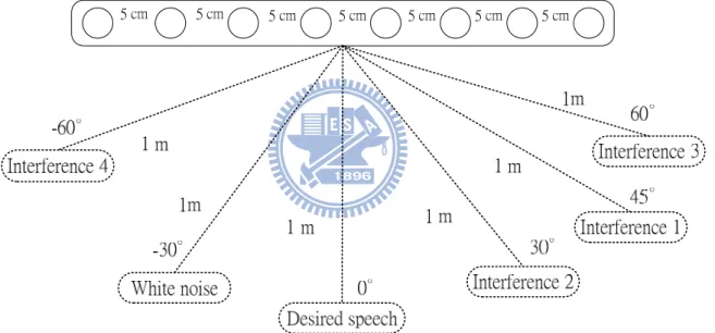
Figure 4-1 Microphone array in real room……….……….………..54

Figure 4-2 Configuration of microphones, desired speech, white noise and interference signals ... 54 

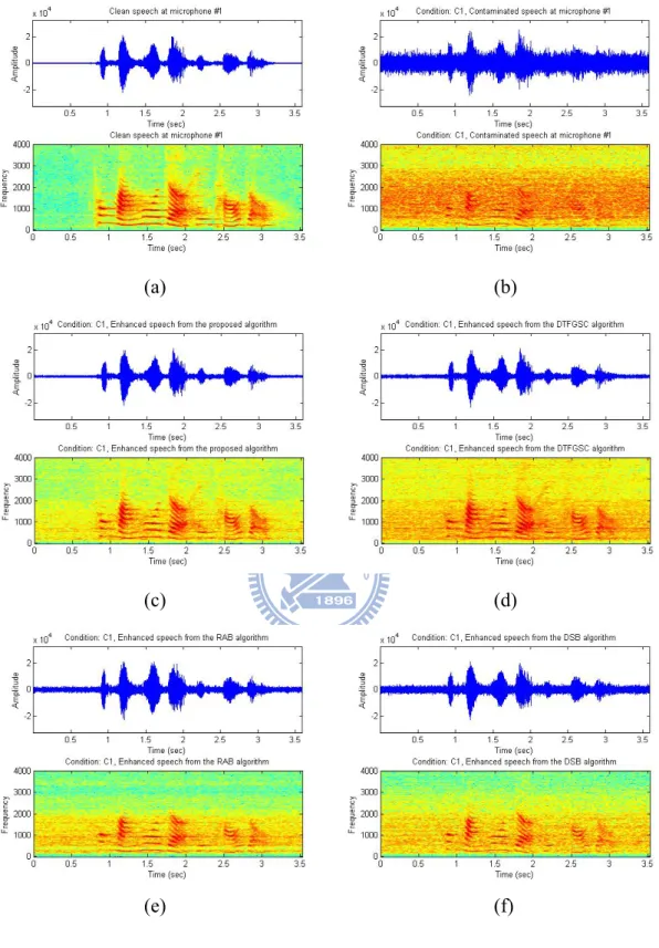
Figure 4-3 Experimental results in real room environment ... 55 

Figure 4-4 Waveforms and spectrograms at condition C1. ... 57 

Figure 4-5 Waveforms and spectrograms at condition C2. ... 58 

Figure 4-6 Waveforms and spectrograms at condition C3. ... 59 

Figure 4-7 Waveforms and spectrograms at condition C4. ... 60 

Figure 4-8 Waveforms and spectrograms at condition C5. ... 61 

Figure 4-9 Microphone array in car ... 63 

Figure 4-10 Car environment ... 63

Figure 4-11 Experimental results in car environment ... 63 

Figure 4-12 Estimation results of state values. ... 69 

Figure 4-13 Configuration of microphones, desired speech, white noise and interference signals ... 71 

Figure 4-14 Simulation results. ... 73 

Figure 4-15 Simulation results. ... 74 

Figure 4-16 Experimental results in real room environment ... 76 

Index

Automatic speech recognition (ASR)………...50

Average SINR (avgSINR)………....52

Blocking matrix (BM)……….………...5

Constant directivity beamformer (CDB)……….………..….2

Delay-and-sum beamformer (DSB)………..……..2

Dual-source transfer-function generalized sidelobe canceller (DTF-GSC)………...51

Fixed beamformer (FB) ...5

Finite impulse response (FIR)…...……….………2

Generalized sidelobe cancellation (GSC)………...4

Hidden markov model (HMM) ………....64

Linearly constrained minimum variance (LCMV)……….……4

Log spectral distortion (LSD)...53

Mel frequency cepstral coefficients (MFCC)………...64

Multiple-input multiple-output (MIMO)...5

Mean square error (MSE)………...37

Minimum variance distortionless response (MVDR)...6

Normalized least-mean-square (NLMS)………..……..5

Power spectrum density (PSD)...31

Reference-signal-based adaptive beamforming (RAB)...51

Root mean square (RMS)………...25

Segmental noise level (segNL)...52

Segmental signal-to-interference-plus-noise ratio (segSINR)………...52

Single-input multiple-output (SIMO) ...14

Sample matrix inversion (SMI)………....36

Second-order extended (SOE) ...6

Short time Fourier transform (STFT)………...12

Singular value decomposition (SVD)………..…….11

Transfer function (TF)………4

Chapter 1

Introduction

Background noise and reverberation could seriously deteriorate the quality of speech signals received by sensors. Speech enhancement algorithms have therefore attracted a great deal of interest in the past three decades. For removing unwanted interference and noise from the desired signal, microphone array processing techniques are widely used. Speech enhancement algorithms using microphone array typically incorporate both spatial and spectral information. Hence, they have the potential to outrun methods using a single microphone where only the spectral information can be used. Among several existing microphone-array-based enhancement algorithms, beamformer is one of the most popular methods and was extensively studied for hands-free speech communication or recognition.

1.1 Overview of Beamformers

In speech communication, if the desired signal and the interfering signals occupy the same frequency band, it is difficult for temporal or spectral filtering methods to

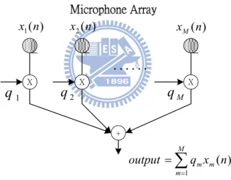
separate the signal from the interferences. However the desired and the interfering signals are usually emitted from different spatial locations. This location difference can be exploited to separate them using a beamformer. A beamformer is an array of microphones which provide spatial information regarding acoustic dynamics of the sources. Typically, a beamformer linearly combines the spatially sampled waveform from each microphone in the same way as the finite impulse response (FIR) filter combines the temporally sampled data. The diagram of a beamformer with M microphones is shown in Fig. 1-1.

In the following, the existing beamformers are explained in two categories: fix beamformers and adaptive beamformers.

) ( 1 n x x₂(n) x_M(n) X X X 1

q

q

2

q

M +

∑

= = M m m mx n q output 1 ) (

Figure 1-1 Diagram of the beamformer

1.1.1 Fix Beamformers

Fix beamformers includes delay-and-sum beamformer (DSB) [1], constant directivity beamformer (CDB) [2-4] and fixed superdirective beamformers [5-7]. They utilize fixed coefficients to achieve a desired spatial response. The DSB is the simplest structure in fixed beamformer and it first compensates for the relative time delay between distinct microphone signals and then sums the steered signal to form a single output. Jan and Flanagan [8] explicitly modeled the transfer function from source to

sensors to replace the simple delay assumption. Further, they extended the DSB concept by introducing the matched filter array beamformer. CDB is designed such that the spatial response is the same over a wide frequency band while the fixed superdirective beamformer attempts to suppress noise coming from all directions without affecting the desired speech signal from a principal direction. Fix beamformers generally assume the desired sound source, interference signals, and noises are slowly varying and at known locations. Therefore, these algorithms are sensitive to steering errors which limit their noises suppression performance and cause the desired signal distortion or cancellation. Furthermore, these algorithms also have limited performance under highly reverberation environments.

1.1.2 Adaptive Beamformers

Instead of using fixed coefficients to suppress noises and interference signals, an adaptive beamformer [9-14] can adaptively forms its directivity beam-pattern to the desired signal and its null beam-pattern to the undesired signals. In the fixed beamformers, the null beam-pattern exists when the noise’s direction is known and remains unchanged. To cope with environmental changes, various adaptive beamformers were proposed to improve the performance. One of the key issues in adaptive beamformers is the sensitivity due to the mismatch between the actual desired signal steering vector and the presumed one [11], [12]. The mismatch can be induced by signal point errors [13], imperfect array calibration [14], or the channel effect (e.g., near-far problem [15], environment heterogeneity [16] and source local scattering [17]). In the presence of these effects, an adaptive beamformer can easily mix up the desired signal and interference components; that is, it suppress the desired signal instead of maintaining distortionless response. This phenomenon is commonly

referred to as signal self-nulling [18]. As a result, much effort has been devoted to the robustness issues [11].

Modifications to adaptive beamformer techniques for robustness were extensively studied. The linearly constrained minimum variance (LCMV) beamformer was proposed in [9] to minimize the array output power under a look-direction constraint. Another popular technique is the generalized sidelobe canceler (GSC) algorithm which essentially transforms the LCMV constrained minimization problem into an unconstrained one [10]. In the last decade, several techniques addressing this problem of the mismatch of the steering vector in the LCMV or GSC structure were developed [19]-[23]. For example, Hoshuyama et al [20] proposed two robust constraints on blocking matrix design. Spriet et al [22] proposed a robust adaptive beamformer called the spatially pre-processed speech distortion weighted multichannel Wiener filter which takes speech distortion into account in its optimization criterion and encompasses the standard GSC as a special case. Further, some ad hoc approaches were discussed to overcome the arbitrary desired signal mismatches, such as the diagonal loading of the sample covariance matrix [24], [25] and the eigenspace-based beamformer [26], [27].

1.1.3 Explicit Transfer Function Modeling for Adaptive beamformers

The other method to mitigate the problem of signal steering vector mismatch for adaptive beamformer is to abandon the delay-only propagation assumption and explicitly model the sound signal propagation from the source to the microphones by an arbitrary transfer function (TF) [28]. Affes and Grenier presented GSC-based near-field beamformer [29] using matched filters with signal subspace tracking. The matched filters which can be identified by the proposed signal subspace tracking

algorithm under the assumption of the FIR model and small displacements of the talker is used to design the fixed beamformer (FB) of the GSC.

Rather than estimating the TF, Gannot et al. [30] proposed the transfer function ratio (TFR) concept and applied to the GSC algorithm. The TFR can be estimated by exploiting the nonstationary characteristics of the desired signal. The suboptimal speech enhancement algorithm that can be implemented by using TFR to design the FB and blocking matrix (BM) of GSC is proposed. Several adaptive beamformer algorithms based on the GSC structure using TF ratio information have been proposed [31]-[33]. Dahl et al. [34] proposed a reference signal based adaptive beamformer which can suppress the nonstationary and stationary noise as well as recover the reverberation at the same time. This method uses FIR based normalized least-mean-square (NLMS) filtering approach to perform noise suppression and speech dereverberation by using pre-recorded speech signals and the desired signal acquired when the environment is quiet. Improvements on the finite number of taps in the FIR filters and relaxation on the disturbance assumption were studied [35]. Huang

et al. [36], [37] treated a microphone array as a multiple-input multiple-output

(MIMO) system and proposed a two-stage procedure for separation and dereverberation of speech signals. The interference signals can be removed by using two microphones with known TFs and the separated reverberant speech can be dereverberated by using the multiple-input/output inverse theorem. However, the stationary noise is neglected in this work and the transfer function of each speech source should be identified in advance during each single-talk interval which also limits its applications in practice.

Most of the early methods of making the adaptive beamformers more robust to the steering vector errors are rather as hoc in that the choice of their parameters or the structural modifications is not directly related to the uncertainty of the steering vector [11]. Recently, Vorobyov et al proposed a new approach to robust adaptive beamforming in the presence of an arbitrary unknown steering vector mismatch [38]. This approach is based on the optimization of worst-case performance. They also showed that the robust minimum variance distortionless response (MVDR) beamformer using worst-case performance optimization can be formulated as a second-order cone program and solved in polynomial time via the interior point method. In further works, [40]-[44], several extensions of the robust MVDR beamformer of [38] have been considered.

1.2 Outline of Proposed Beamformers

The objective of this dissertation is to provide satisfactory beamfromer performance and robustness to background noise and channel effects using a uniform linear microphone array. Two adaptive beamformers, TFR-based adaptive beamformer and robust adaptive beamformer based on the second-order extended

(SOE) H∞ filter, which can be categorized into Section 1.1.3 and 1.1.4 are proposed in

this dissertation.

1.2.1 Transfer Function Ratio-Based Adaptive Beamformer

The first beamformer, TFR-based adaptive beamformer, belongs to the category of Section 1.1.3 since a pre-training procedure is needed to explicitly model the TFR. The TFR-based adaptive beamformer is designed to extract the desired speech signal

while attenuating multiple competing speeches in a reverberant and noisy environment. The proposed method uses TFR beamformer and multi-channel adaptive filter algorithm to perform speech enhancement. The TFR beamformer is utilized to block the major component of the interference signals and the channel effect of the desired speech is adjusted by the TFR information. The residual noise signals from

the TFR beamformer output are suppressed by the constrained H∞ filter. In addition,

the virtual sound source concept is proposed to simplify the treatment for multiple competing speeches.

1.2.2 Robust Adaptive Beamformer Based on the Second-Order

Extended H∞ Filter

The second beamformer, robust adaptive beamformer based on the SOE H∞ filter,

belongs to the category of Section 1.1.4 since the beamformer structure is based on the robust MVDR beamformer of [38] which assumes that the transfer function is a

delay-only propagation with an uncertainty. This dissertation develops the SOE H∞

filter for the implementation of the robust MVDR beamformer and the SOE H∞ filter

is derived by the game theory approach. The estimation criterion in the SOE H∞ filter

design is to minimize the worst possible effects of the disturbance signals on the signal estimation errors without priori knowledge. The proposed beamformer is compared with the existing robust adaptive beamformer based on the SOE Kalman filter.

1.3 Contribution of this Dissertation

algorithms for speech enhancement. This dissertation proposes two adaptive beamformers, TFR-based adaptive beamformer and robust adaptive beamformer

based on the SOE H∞ filter.

1. Speech enhancement in a reverberant noisy environment with multiple competing speech signals is still a difficult problem. The challenge lies in the coexistence of spatial interference from competing sources and temporal echoes due to room reverberation in the received signals. In the TFR-based adaptive

beamformer, a novel beamformer structure is proposed and the constrained H∞

filter is applied to overcome the problem above. In addition, the virtual sound source concept is proposed to simplify the multiple competing speech signals and explain the component blocked by the TFR beamformer.

2. Many efforts have been considered to expand the H∞ filter to different domains

and to improve performance. However, no work has been done on considering the second-order extended case similar to that of the SOE Kalman filter. In this

dissertation, a SOE H∞ filter for a nonlinear discrete time system is derived based

on the game theory approach. A numerical example is given to compare the

proposed SOE H∞ filter with the first-order extended H∞ filter, and the SOE

Kalman filter.

3. The robust MVDR beamformer of [38] has been implemented by the SOE Kalman filter [44]. However, the assumptions of the SOE Kalman filter about the

disturbance limit the beamformer performance. The proposed SOE H∞ filter is

applied to implement the robust MVDR beamformer of [38] for speech enhancement to improve the issue above.

1.4 Dissertation Organization

The remainder of this dissertation is organized as follows. The TFR-based adaptive beamformer is introduced in Chapter 2. Chapter 3 presents the robust adaptive

beamformer based on the SOE H∞ filter. Also, the SOE H∞ filter solution of a general

nonlinear discrete-time system is provided and the detail derivation is given in the Appendix I-IV. Chapter 4 shows the experimental results in both simulated room and real environment. Finally, conclusion and future work are drawn in Chapter 5.

Chapter 2

Transfer Function Ratio-Based Adaptive

Beamformer

2.1 Introduction

Speech enhancement in the presence of multiple competing speech signals under a reverberant and noisy environment is still a difficult problem. The challenge lies in the coexistence of spatial competing sources and temporal echoes from room reverberation [74]. This dissertation considers speech enhancement problem under multiple speech sources in a reverberant and noisy environment condition and we focus on reconstructing the desired speech while suppressing competing speech sources and stationary noise. To deal with this problem, the most commonly used algorithm is the LCMV [9] algorithm where the adaptive weight is trained to satisfy certain constraints for a set of directions while minimizing the array response in all other directions. Therefore, the adaptive weight in LCMV-based structure [9], [34] has two objectives: to minimize the interference signal and noises, and to equalize the channel effect of the desired speech (e.g. room acoustics). However, in practical environment, existing adaptive filter algorithms (e.g.

Hence, it serves as the motivation for this work to separate these two objectives using different beamformer weights.

This dissertation proposes a two-stage speech enhancement algorithm using the TFR beamformer and the multi-channel adaptive filter algorithm. As discussed in Section 1.1.3, the TFR is originally used to design the FB and BM of GSC [30] and this work uses it to equalize the channel effect and block the interference signals. In channel equalization part, the channel effect of the desired speech is adjusted by the TFR information. In noise suppression part, the TFR beamformer is employed to reduce certain noise level in advance. In multiple competing speech sources environment, it is cumbersome and impractical to analyze the TFR of each competing speech source. Hence, the virtual sound source perspective explained by singular value decomposition (SVD) method is proposed to simplify the complexity of multiple interference signals environment. The TFR beamformer can be considered a pre-filter to remove the major component of the virtual sound source first and the residual noise from TFR beamformer output can be suppressed by multi-channel adaptive filter. However, the residual noise signals could be nonstationary or hard to model ,and common adaptive filter algorithms (e.g. NLMS algorithm or Kalman filter) may not completely characterize uncertainty under the complexity of acoustic dynamics [35], [46], [47], Therefore, the assumption of bounded disturbances could be a better strategy than others such as certain statistical properties.

Hence, this dissertation adopts the H∞ filter as the multi-channel adaptive filter since it

makes no further assumption regarding the disturbances and can be more robust to the model uncertainty problems [48].

The remainder of this chapter is organized as follows. Section 2.2 describes the problem formulation and the virtual sound source concept. Section 2.3 introduces the proposed system architecture and the performances of each noise cancellation block are also analyzed. The method to estimate the TFR information is presented in Section 2.4.

Finally, the summary is given in Section 2.5.

2.2 Problem Formulation

2.2.1 Problem Description

Consider P speech sources and M microphones in the reverberant and noisy environment (M > P). The received signal of the m-th microphone at discrete-time index t can be written as:

∑

= + ⊗ = P p m p mp m t a t s t n t x 1 ) ( ) ( ) ( ) ( (2-1)

where each symbol in (2-1) represents:

⊗ convolution operation;

) (t

a_mp the transfer function from the p-th sound source to the m-th microphone;

) (

1 t

s the desired speech signal;

) ( ~ ) ( 2 t s t

s _P the nonstationary interfering speech signals (competing speech signals);

) (t

n_m the (directional or omni-directional) stationary noise of the m-th microphone.

Typically, the transfer function a_mp(t) is assumed to be time-invariant over the

observation period. In this dissertation, the competing speech signals, s₂(t)~s_P(t), are

regarded as interference signals. Applying the short time Fourier transform (STFT) operation to (2-1) yields:

( )

∑

= + = P p m p mp m k A S k N k X 1 , ) , ( ) ( ) , ( ω ω ω ω (2-2)

( )

k,ω

N_m are the STFT of x_m(t), )s_p(t and )n_m(t , respectively. A_mp(ω) is the

time-invariant transfer function from the p-th source to the m-th microphone. The objective of this work is to reconstruct the desired speech signal from the received contaminated signals, while suppressing the nonstationary interfering speech signals and the stationary noise signals in a reverberant environment.

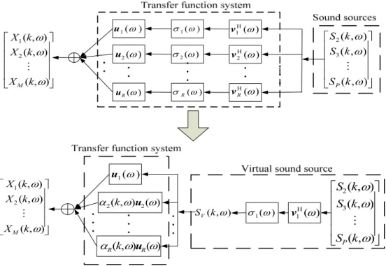
2.2.2 Virtual Sound Source Perspective

It is impractical to estimate the transfer function for each interference signal in real practice. To simplify the complexity involved in multiple interference signals, a virtual sound source perspective is proposed. The idea of virtual sound source comes from that the multiple interference signals may be able to be transferred to one virtual sound source. When the desired speech signal and the stationary noise are absent, the received microphone signal can be expressed as the matrix form:

) , ( ) ( ) , ( _{I I} I k ω ω S k ω X =A (2-3) where ) 1 ( 3 2 2 23 22 1 13 12 I 1 ) 1 ( 3 2 I 1 2 1 I ) ( ) ( ) ( ) ( ) ( ) ( ) ( ) ( ) ( ) ( ) , ( ) , ( ) , ( ) , ( , ) , ( ) , ( ) , ( ) , ( − × × − × ∈ ⎥ ⎥ ⎥ ⎥ ⎦ ⎤ ⎢ ⎢ ⎢ ⎢ ⎣ ⎡ = ∈ ⎥ ⎥ ⎥ ⎥ ⎦ ⎤ ⎢ ⎢ ⎢ ⎢ ⎣ ⎡ = ∈ ⎥ ⎥ ⎥ ⎥ ⎦ ⎤ ⎢ ⎢ ⎢ ⎢ ⎣ ⎡ = P M MP M M P P P P M M C A A A A A A A A A C k S k S k S k C k X k X k X k ω ω ω ω ω ω ω ω ω ω ω ω ω ω ω ω ω ω L M M M L M M A S X

Assume the rank of the transfer function matrix A_I(ω) is R and A_I(ω) can be

) ( )V )D( U( ) ( A_I ω = ω ω Η ω (2-4) where

[

]

[

]

( ) R R R R P R R M R C C C × × − × ∈ ⎥ ⎥ ⎥ ⎥ ⎦ ⎤ ⎢ ⎢ ⎢ ⎢ ⎣ ⎡ = ∈ = ∈ = ) ( σ 0 0 0 ) ( σ 0 0 0 ) ( σ ) ( ) ( ) ( ) ( ) ( ) ( 2 1 1 2 1 2 1 ω ω ω ω ω ω ω ω ω ω ω ω L M O M M L L L L ) D( ) V( ) U( v v v u u u ) (

σ_r ω are the nonzero singular values of A_I(ω) with σ₁(ω)≥σ₂(ω)≥_L≥σ_R(ω)>0.

) (

r ω

v and u_r(ω) are the input and output singular vectors of A_I(ω) respectively

which construct the interference subspace. The idea of virtual sound source is characterized as follows. From (2-4), equation (2-3) can be rewritten as:

(

( ) ( , )

)

( , ) ) , ( ) ( ) ( ) ( ) , ( _I 1 I ω ω ω ω ω ω ω σ ω k S k k k V V V i i R i i Δ A S v u X + = = Η =

∑

_(2-5) where ) , ( ) ( ) ( σ ) , ( ) ( ) ( σ ) , ( ) ( ) , ( ) , ( ) , ( ) , ( ) , ( , ) ( ) ( ) ( ) ( ) ( ) , ( ) ( ) ( σ ) , ( I 1 1 I H 2 2 1 1 2 1 I 1 1 ω ω ω ω ω ω ω α ω ω α ω ω ω ω ω ω ω ω ω ω ω ω ω k k k k k k k k A A A k k S H i i i R i i i MV V V V MV V V V H V S v S v u Δ u A S v = = ⎥ ⎥ ⎥ ⎥ ⎦ ⎤ ⎢ ⎢ ⎢ ⎢ ⎣ ⎡ Δ Δ Δ = = ⎥ ⎥ ⎥ ⎥ ⎦ ⎤ ⎢ ⎢ ⎢ ⎢ ⎣ ⎡ = =

∑

= M M

Observing (2-5), we can find that the MIMO acoustic system of (2-3) is treated as the single-input multiple-output (SIMO) acoustic system. The single input is the virtual sound

) ( 1 ω Η v ) (ω Η R v ) ( 1 ω σ ) ( 2 ω σ ) (ω σR ) ( 2Η ω v ) ( 1 ω u ) ( 2 ω u ) (ω R u ) , ( ) , ( ) , ( 2 1 ⎥ ⎥ ⎥ ⎥ ⎦ ⎤ ⎢ ⎢ ⎢ ⎢ ⎣ ⎡ ω ω ω k X k X k X M M ⎥ ⎥ ⎥ ⎥ ⎦ ⎤ ⎢ ⎢ ⎢ ⎢ ⎣ ⎡ ) , ( ) , ( ) , ( 3 2 ω ω ω k S k S k S P M ) ( 1Η ω v ) ( 1 ω σ ⎥ ⎥ ⎥ ⎥ ⎦ ⎤ ⎢ ⎢ ⎢ ⎢ ⎣ ⎡ ) , ( ) , ( ) , ( 3 2 ω ω ω k S k S k S P M ) , (kω SV ) ( 1 ω u ) ( ) , ( 2 2 ω ω α k u ) , ( ) , ( ) , ( 2 1 ⎥ ⎥ ⎥ ⎥ ⎦ ⎤ ⎢ ⎢ ⎢ ⎢ ⎣ ⎡ ω ω ω k X k X k X M M ) ( ) , ( ω ω αR k uR

Figure 2-1 Illustration of virtual sound source transformation

which in turn is scaled by the maximum singular value σ₁(ω . The TF of the virtual )

sound source consists of two parts, time-invariant part A_V(ω) and time-varying part

) ,

(k ω

V

Δ . This dissertation considers that A_V(ω) is constructed by the highest gain

output direction u₁(ω) and Δ_V(k,ω) is the linear combination of u₂(ω)~u_R(ω) with

time-varying coefficients α_i(k,ω). The transformation from multiple sound sources to

the virtual sound source is illustrated in Fig. 2-1.

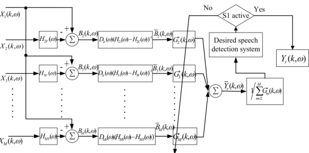
2.3 System Architecture

The proposed system architecture of the TFR-based adaptive beamformer is shown in Fig. 2-2. The proposed beamformer uses the TFR-based beamformer to block the principal part of the virtual sound source and the residual noise signals from the TFR-based beamformer outputs are suppressed by the multi-channel adaptive filter.

Σ Σ Σ ) ( 2Vω H ) ( 3V ω H ) (ω MV H + -+ -+ -Σ ) , ( 2kω B ) , ( 3kω B ) , (kω BM 1 2 21 2r(ω)(H(ω)−HV(ω))− D 1 3 31 3( )( ( ) ( )) − − ω ω ω V r H H D 1 1() ()) )( (_{ω ω− ω}− MV M Mr H H D ) , ( 2 kω G∗ ) , ( 2kω B ) , ( 3 kω G∗ ) , ( 3kω B ) , (kω BM ) , (kω GM∗

∑

= ∗ M m mk G 2 ) , ( 1 ω ) , (kω Y_r ) , ( 1kω X ) , ( 2 kω X ) , ( 3kω X ) , (kω X_M ) , (kω Yr Desired speech detection system S1 active No _Yes

Figure 2-2 The system architecture of the TFR-based adaptive beamformer

According to Section 2.2.2, equation (2-2) can be written as

(

( ) ( , )

)

( , ) ( , ) ) , ( ) ( ) , ( ) , ( ) ( ) , ( ) ( ) , ( ) , ( ) ( ) , ( 1 1 2 1 1 1 ω ω ω ω ω ω ω ω ω ω ω ω ω ω ω k N k S k A k S A k N k S A k S A k N k S A k X m V mV mV m m P p p mp m m P p mp p m + Δ + + = + + = + =

∑

∑

= = (2-6)

For the virtual sound source components, we consider A_mV(ω)S_V(k,ω) and

) , ( ) , (k ω S_V k ω mV

Δ to be the principal part and residual part respectively, since A_V(ω)

is the highest gain output direction of the transfer function matrix A_I(ω) and

) , ( )

(ω S k ω

A_{mV V} is constructed by the principal interference subspace. If the number of

sound sources is two, i.e., P=2, then the residual part is zero.

2.3.1 Transfer Function Ratio Beamformer

A TFR beamformer consists of two microphones. In this work, M received microphone

supposed that the TFRs defined in (2-7) have been identified using the method introduced

in Section2.4. The TFRs for the desired speech and virtual sound source are defined as

M m A A H A A H mV V mV m m _{( )}, 2,3, , ) ( ) ( , ) ( ) ( ) ( 1 1 11 1 = = _ω = L ω ω ω ω ω (2-7)

First, this dissertation employs the TFR of the virtual sound source to remove the principal part of the virtual sound source for each microphone pair:

M m k S k A A k k N A A k N k S A A A A A k S k A A k k N A A k N k S A A A A k X A A k X k B V mV mV V V m mV V mV V m m V mV mV V V m mV V m mV V m mV V m , , 3 , 2 for ) , ( ) , ( ) ( ) ( ) , ( ) , ( ) ( ) ( ) , ( ) , ( ) ( ) ( ) ( ) ( ) ( ) , ( ) , ( ) ( ) ( ) , ( ) , ( ) ( ) ( ) , ( ) , ( ) ( ) ( ) ( ) ( ) , ( ) ( ) ( ) , ( ) , ( 1 1 1 1 1 1 1 11 1 1 1 1 1 1 1 1 11 1 1 L = ⎟⎟ ⎠ ⎞ ⎜⎜ ⎝ ⎛ Δ − Δ + − + ⎟⎟ ⎠ ⎞ ⎜⎜ ⎝ ⎛ − = ⎟⎟ ⎠ ⎞ ⎜⎜ ⎝ ⎛ Δ − Δ + − + ⎟⎟ ⎠ ⎞ ⎜⎜ ⎝ ⎛ − = ⎟⎟ ⎠ ⎞ ⎜⎜ ⎝ ⎛ − = ω ω ω ω ω ω ω ω ω ω ω ω ω ω ω ω ω ω ω ω ω ω ω ω ω ω ω ω ω ω ω ω ω ω (2-8)

Equation (2-8) means that the spatial null is placed toward the direction of the principal part of the virtual sound source by using two microphones. If the number of sound

sources is two (Δ_mV(k,ω)=0), equation (2-8) means that the spatial null is placed toward

the single competing speech directly. The output of TFR beamformer B_m(k,ω) consists

of 3 terms: distorted desired speech signal, stationary noise and residual virtual sound

source. Since the TFRs, H_m1(ω) and H_mV(ω) , are known and we assume

)) ( )

(

(H_m1 ω −H_mV ω is non-zero. To mitigate the distortion on the desired speech signal,

equation (2-8) is multiplied by 1 1( ) ( )) )( (_{ω ω − ω} − mV m mr H H D :

1 1 1 1 1 1 1 1 1 1 1 1 )) ( ) ( )( ( ) , ( ) , ( ) ( ) ( ) , ( )) ( ) ( )( ( ) , ( ) ( ) ( ) , ( ) , ( ) ( )) ( ) ( )( ( ) , ( ) , ( − − − − ⎟⎟ ⎠ ⎞ ⎜⎜ ⎝ ⎛ Δ − Δ + − ⎟⎟ ⎠ ⎞ ⎜⎜ ⎝ ⎛ − + = − = ω ω ω ω ω ω ω ω ω ω ω ω ω ω ω ω ω ω ω ω ω ω mV m mr V mV mV V V mV m mr m mV V r mV m mr m m H H D k S k A A k H H D k N A A k N k S A H H D k B k B (2-9) where M r H H A A D _{m r} m r mr ( )( ( )) 1,2, , ) ( ) ( ) ( -1 1 1 1 1 _{= = L} = ω ω ω ω ω ) (ω mr

D is used to adjust the desired speech signal distortion to the same reference and r

is the reference microphone number selected.

The noise components of output signal B_m(k,ω) still contain the residual part of the

virtual sound source and stationary noise (the last two terms of the right side of (2-9)), and hence the multi-channel adaptive filter is employed here to minimize the noise in

) ,

(k ω

B_m . Let us sum all the output signals B_m(k,ω) with the weighting function

) , (k ω G_m : 1 1 1 1 2 1 1 1 1 2 2 1 1 2 2 )) ( ) ( )( ( ) , ( ) , ( ) ( ) ( ) , ( ) , ( )) ( ) ( )( ( ) , ( ) ( ) ( ) , ( ) , ( ) , ( ) , ( ) ( ) , ( ) , ( ) , ( ) , ( ) , ( − = ∗ − = ∗ = ∗ ∗ ∗ − ⎟⎟ ⎠ ⎞ ⎜⎜ ⎝ ⎛ Δ − Δ + − ⎟⎟ ⎠ ⎞ ⎜⎜ ⎝ ⎛ − + = + + =

∑

∑

∑

ω ω ω ω ω ω ω ω ω ω ω ω ω ω ω ω ω ω ω ω ω ω ω ω ω mV m mr V mV mV V V M m m mV m mr m mV V M m m M m m r M M r H H D k S k A A k k G H H D k N A A k N k G k G k S A k B k G k B k G k Y _L (2-10)

where * represents the complex conjugation. The noise components can be cancelled if ) , ( ) , ( ) , ( ) , (k ω k ω =−G₂ k ω Z₂ k ω Η _Z G (2-11)

[

]

[

]

1 1 1 1 1 1 1 1 3 3 2 )) ( ) ( )( ( ) , ( ) , ( ) ( ) ( ) , ( )) ( ) ( )( ( ) , ( ) ( ) ( ) , ( ) , ( ) , ( ) , ( ) , ( ) , ( ) , ( ) , ( 1 ) , ( − − Τ Τ − ⎟⎟ ⎠ ⎞ ⎜⎜ ⎝ ⎛ Δ − Δ + − ⎟⎟ ⎠ ⎞ ⎜⎜ ⎝ ⎛ − = = = = ω ω ω ω ω ω ω ω ω ω ω ω ω ω ω ω ω ω ω ω ω ω ω mV m mr V mV mV V V mV m mr m mV V m M M H H D k S k A A k H H D k N A A k N k Z k Z k Z k k G k G k k G L L Z G

The solution of G(k,ω) can be found by using adaptive algorithm suggested in Section

2.3.2 when S₁(k,ω) is silent (desired speech inactive periods). Once the weight vector

) ,

(k ω

G is obtained, the beamformer output can be given as:

∑

= ∗ = _M m m r r k G k Y k Y 2 ) , ( ) , ( ) , ( ω ω ω (2-12)

2.3.2 Multi-channel Adaptive Filter

For the real environment, it is unlikely to remove the noise components of (2-10)

completely and hence the output signal Y_r(k,ω) can be expressed as:

) , ( ) , ( ) , ( ) ( ) , ( 2 1 1 ω ω ω ω ω A S k G k e k k Y M _n m m r r =

∑

+ = ∗ _(2-13)

where e_n(k,ω) is the residual noise and it is anticipated that the desired speech signal

components are dominant compared to the residual noise. Therefore, equation (2-12) can be written as:

∑

= ∗ + = _M m m n r r k G k e k S A k Y 2 1 1 ) , ( ) , ( ) , ( ) ( ) , ( ω ω ω ω ω (2-14)

According to (2-11), the error signal at frequency ω and frame k can be defined as:

) , ( ) , ( ) , ( ) , ( ) , ( ω ₂ ω ₂ ω ω ω ε_Z k =−G k Z k −GΗ k Z k (2-15)

To minimize the error signal ε_Z(k,ω), the optimal set of filter coefficients vectors )

,

(k ω

G can be found using the formula:

[

( , ) ( , )

]

minEε_Z k ω ε_Z k ω

G

∗ _(2-16)

where E

[]

⋅ is the expectation. Observing (2-12), the weight-and-sum output Y_r(k,ω) is

divided by

∑

= ∗ M m m k G 2 ) ,

( ω to be the beamformer output Y_r(k,ω). Hence, to prevent the

term e_n(k,ω) in (2-14) from being amplified by

∑

= ∗ M m m k G 2 ) ,

( ω and a constraint is added

into (2-16) as:

[

]

O G ( , ) subject to ) , ( ) , ( min ω β ω ε ω ε k k k E _{Z Z} Q Η ∗ = (2-17) where ₌

[

_{1 1 1}

]

Τ_∈R(M−2)×1 L

O and β is a constant larger than zero to ensure the

value of

∑

= ∗ M m m k G 2 ) ,

( ω not to amplify the residual noise e_n(k,ω) in (2-14). H2-optimal

estimators (i.e. least-square based), such as the Wiener filter or Kalman filter, which minimize the expected estimation error energy and yield maximum-likelihood estimates are usually used to solve the optimization problem of (2-17). However, the least-square-based filters have some assumption about the disturbances. For example, Kalman filter assumes that signal generating processes have known dynamics and that the disturbances have known statistical properties. These assumptions may limit the beamformer performance. Among the classic adaptive filters, the NLMS algorithm is one of the most popular methods and widely used since it can be implemented easily. The NLMS algorithm solution of (2-17) is given by:

(

)

O O Z Z O Z G G _{Η Η} ∗ ∗ + + + = + μ ω ω ω με ω ω ε λ ω ω ) , ( ) , ( ) , ( ) , ( ) , ( ) , ( ˆ ) , 1 ( ˆ k k k k k k k Z N _(2-18)

O

G ( , )

) ,

( ω β ω

ε_N k _{= −} Η k _{. However, the modeling error of G(k,ω) or the nonstationary}

signals in Z(k,ω) may influence the performance and convergence rate of the NLMS

algorithm. Therefore, the H∞ filter is applied here for the optimization problem. Because

the disturbances in the H∞ estimation can be arbitrary but bounded signals and the H∞

filter was shown to be more robust than other least-square-based methods [35], [46]-[49].

To apply the H∞ filter, the constrained minimization problem of (2-17) is casted as a

state-space model: State equation: ) , 1 ( ) , (k ω =G k− ω G (2-19) Measurement equation: ⎥ ⎦ ⎤ ⎢ ⎣ ⎡ + ⎥ ⎦ ⎤ ⎢ ⎣ ⎡ = ⎥ ⎦ ⎤ ⎢ ⎣ ⎡− Η Η ∗ ) , ( ) , ( ) , ( ) , ( ) , ( 2 1 2 ω ω ω ω β ω k v k v k k k Z G O Z (2-20)

The measurement equation can be written as: ) , ( ) , ( ) , ( ) , (k ω k ω G k ω V k ω M =_ZΗ + _(2-21) where ⎥ ⎦ ⎤ ⎢ ⎣ ⎡ = ⎥ ⎦ ⎤ ⎢ ⎣ ⎡ = ⎥ ⎦ ⎤ ⎢ ⎣ ⎡− = ∗ Η Η _Η ) , ( ) , ( ) , ( , ) , ( ) , ( , ) , ( ) , ( 2 1 2 ω ω ω ω ω β ω ω k v k v k k k k Z k V O Z M Z (2-22) ) , ( 1 k ω

v and v₂(k,ω) are the beamformer residual noise and constraint noise,

respectively. The H∞ filter makes no assumption about the statistics of the noise v1(k,ω)

and v₂(k,ω) and is interested not necessarily in the estimation of G(k,ω) but in the

estimation of some arbitrary linear combination of G(k,ω), i.e.,

) , ( ) , (k ω G k ω T =C (2-23)

the estimate of initial state G(0,ω) is denoted by Gˆ(0,ω). The design criterion of the

H∞ filter is to find Tˆ(k,ω) that minimizes T(k,ω)−Tˆ(k,ω) for any v₁(k,ω) ,

) , (

2 k ω

v and G(0,ω). The performance index J can be defined as:

∑

∑

− = − = − − + − − = ₁ 0 2 ) , ( 2 ) (0, 1 0 2 ) , ( 1 1 ( , ) ) , 0 ( ˆ ) , 0 ( ) , ( ˆ ) , ( N k k N k k k k k J ω ω ω ω ω ω ω ω R P S V G G T T (2-24)

where the notation x(k,ω)_S2_(k,ω) is defined as the square of the weighted (by S(k,ω))

L2 norm of x(k,ω), i.e., x(k,ω)_S2_(k,ω) = xΗ(k,ω)S(k,ω)x(k,ω). The matrices P(0,ω),

) ,

(k ω

R and S(k,ω) are symmetric positive definite matrices chosen by the user based

on the specific problem. To simplify the analysis and clarify the notation, we assume the

weighting matrices,R(k,ω) and S(k,ω), are the same at each frame and each frequency,

i.e., they are independent of frame and frequency. Hence, equation (2-24) can be reformulated as

∑

∑

− = − = − − + − − = ₁ 0 2 2 ) (0, 1 0 2 1 1 ( , ) ) , 0 ( ˆ ) , 0 ( ) , ( ˆ ) , ( N k N k k k k J R P S ω ω ω ω ω ω V G G T T (2-25)

The direct minimization of J is not tractable, so instead, a performance bound γ is

selected and Tˆ(k,ω) is computed to satisfy

γ

<

sup J (2-26)

where sup represents supremum. The formulation of (2-26) shows that the H∞ optimal

estimators guarantee the smallest estimation error energy over all possible disturbances

(G(0,ω)−Gˆ(0,ω) and V(k,ω)) of finite energy. They are over-conservative but have a

) , (

ˆ _{k ω}

T that minimizes the supremum of the cost function J. Hence, the H∞ filter can be

interpreted as a minmax problem where the estimator strategy Tˆ(k,ω) plays against the

exogenous inputs V(k,ω) and the uncertainty of the initial state G(0,ω).Therefore, the

performance criterion is equivalent to

(

)

∑

− = ⎥⎦ ⎤ ⎢⎣ ⎡ _{− −} + − − = − − 1 0 2 2 2 ) (0, ) , 0 ( , ˆ 1 1 ) , ( ) , ( ˆ ) , ( ) , 0 ( ˆ ) , 0 ( max min N k k k k J R S P ω γ ω ω ω ω γ ω ω V T T G G G V T (2-27) Since V(k,ω)₌M(k,ω)_−ZΗ(k,ω)G(k,ω)_{, )T(k,ω)=CG(k,ω and} ) , ( ) , (k ω G k ω

T =C , equation (2-27) can be rewritten as:

∑

− = Η ⎥⎦ ⎤ ⎢⎣ ⎡ _⎟ ⎠ ⎞ ⎜ ⎝ ⎛ ₋ − − + − − = − − 1 0 2 2 2 ) (0, ) , 0 ( , ˆ 1 1 ) , ( ) , ( ) , ( ) , ( ˆ ) , ( ) , 0 ( ˆ ) , 0 ( max min N k k k k k k J R S P Z ω ω ω γ ω ω ω ω γ ω ω G M G G G G G M G (2-28) where S=CΗSC.

According to [48], the H∞ solution can be given as:

[

1 _{( , ) ( , )} 1 _{( , ) ( , )}

]

1 _{( , )} 1 ) , ( ) , ( =P I− −SP +Z R−ZΗ P − Z R− K k ω k ω γ k ω k ω k ω k ω k ω (2-29)

[

( , ) ( , )ˆ( , )

]

) , ( ) , ( ˆ ) , 1 ( ˆ _{k ω G k ω k ω M k ω k ω G k ω} G _{+ = +K −Z}Η _(2-30)

[

_{1 1}

]

1 ) , ( ) , ( ) , ( ) , ( ) , 1 (k+ ω =P k ω I−γ−SP k ω +Z k ω R−ZΗ k ω − P (2-31)

where I is the identity matrix. The H∞ solution above can also be used to solve the

unconstrained minimization problem of (2-16) by setting:

[

( , )

]

, ( , )

[

( , )

]

) ,

(k ω = −Z₂∗ k ω Η k ω = ZΗ k ω

M Z (2-32)

For the proposed multi-channel adaptive filter, M(k,ω) and ZΗ(k,ω) are set as (2-32)

∑

= ∗ M m m k G 2 ) ,

( ω is less than one after k~ times of adaptation, M(k,ω) and ZΗ(k,ω) will

be set as (2-22). Theoretically, if

∑

= ∗ M m m k G 2 ) ,

( ω is less than one, the value of β should be

set as a constant close to zero to prevent the constrained value from being far away from

the optimal solution. However, there is no such restriction of β in the proposed

architecture, since the residual noise e_n(k,ω) is divided by

∑

= ∗ M m m k G 2 ) , ( ω to be the beamformer output.

2.3.3 The Analysis of TFR Beamformer and Multi-channel Adaptive Filter

In this section, the performances of the individual noise cancellation block (B_m(k,ω)

and Y_r(k,ω)) are analyzed. To analyze the performances, the image method [50] is used

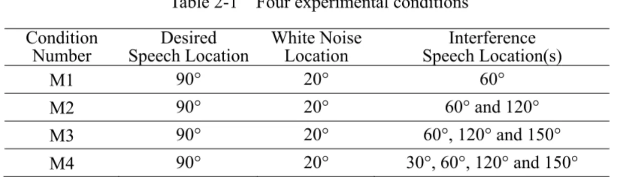
here to simulate the room impulse responses. The simulated room size is 4.5 m × 3.3 m × 4.2 m and the reverberation time is 0.14 second simulated by 532-taps FIR filter. A uniform linear microphone array with eight microphones placed at a distance of 0.7 m from the wall is used for the simulation. The distance between adjacent microphones is 6 cm and the sampling rate is 8 kHz. The directional sources are placed in front of the array from angle 0° to 180° with a distance of 1.5 m from the midpoint of the array. Four different conditions listed in Table 2-1 are considered to demonstrate the performances of each noise cancellation block. To compare the performances of the NLMS algorithm and

Table 2-1 Four experimental conditions Condition

Number Speech LocationDesired White Noise Location Speech Location(s) Interference

M1 90° 20° 60°

M2 90° 20° 60° and 120°

M3 90° 20° 60°, 120° and 150°

the H∞ filter, the multi-channel adaptive filter is implemented by both methods. The STFT

size is 256 with 80 shift samples and 16 zero padding samples. The parameters of λ , μ,

β and γ are in (2-18), (2-18), (2-20) and (2-26) set to 0.3, 1, 2 and 10. The adaptation

number k~ is set to 20. In this simulation, the length of the impulse responses (532) is

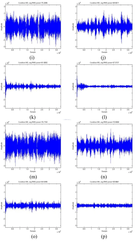
longer than 256. Therefore, the modeling error exists in this simulation. Fig. 2-3 shows

the received signal and the outputs of each noise cancellation block (B₂(k,ω) and

) , (

1 k ω

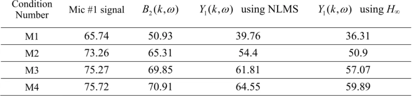
Y ) at four different conditions when the desired speech signal is inactive and Table

2-2 shows the average root mean square (RMS) power at different stage. The average RMS power is defined as:

∑

∑

= = ⎟ ⎟ ⎠ ⎞ ⎜ ⎜ ⎝ ⎛ + = N k L l kL l y L N 1 1 2_{( )} 1 10 log 20 1 avg.RMS (2-33)

where L denotes the length of the frame; k is the frame number and y is the input signal.

Observing the TFR beamformer output (B₂(k,ω)) in Fig. 2-3, we can find that the TFR

beamformer can reduce certain interference parts especially when the interference speech number (P) is small. However, the residual virtual sound source defined in (2-8) may not be relatively small when the number of interference sources becomes large. This is because the TFR beamformer only consists of two microphones and it can only place one null space toward one direction which limits the performance. As can be seen from Fig.

2-3, the H∞ filter can reduce more noise signals than the NLMS algorithm. Since the H∞

filter minimizes the worst possible effects of the disturbances on the estimation error of

) , (k ω

G . Characterizing uncertainty under the complexity of acoustic dynamics is

difficult, so the best strategy may be just to assume that the disturbance is bounded. In addition, the residual virtual sound source may influence the convergence rate of the

NLMS algorithm since it is nonstationary signal. Therefore, this work adopts the H∞ filter

(a) (b)

(c) (d)

(e) (f)

(i) (j)

(k) (l)

(m) (n)

(o) (p)

Figure 2-3 Waveforms of the simulation results (a), (e), (i), (m): received Mic#1 signal at four conditions ;

(b), (f), (j), (n): B₂(k,ω) at four conditions;

(c), (g), (k), (o): Y₁(k,ω) using NLMS algorithm at four conditions;

(d), (h), (l), (p): _Y1(_k,_ω)

ss using H∞ filter at four conditions;

outputs. More comparisons between the H∞ filter and least-square-based filters can be

referred to [35], [46]-[49]. Except the advantage of the H∞ filter, there is also an

advantage of the proposed beamformer architecture. Unlike the standard weight-and-sum beamformer architecture where the beamformer output is obtained by weighting and

summing signals fromdifferent microphones, the proposed architecture makes the

weight-and-sum output Y₁(k,ω) divide by

∑

= ∗ M m m k G 2 ) ,

( ω to be the beamformer output

and it is different from the standard weight-and-sum beamformer architecture. Hence, if

∑

= ∗ M m m k G 2 ) ,

( ω is larger than one, the noise components in (2-10) can be attenuated again

using (2-12).

To test the performance of the proposed structure, one more simulation is performed.

Consider the M3 condition and the goal of this simulation is to find the weight Gˆ(k,ω)

that minimizes ε_Z(k,ω) during noise-only-periods. Two beamformer structures shown

in Table 2-3 are used for comparison. The first one is the standard weight-and-sum structure and the second one is the proposed beamformer structure. Fig. 2-4 shows the

simulation results of both beamformers with NLMS algorithm and the H∞ filter. The

initial condition of Gˆ(k,ω) for the NLMS algorithm and the H∞ filter are the same. The

parameters of λ , μ , β and γ are in (2-18), (2-18), (2-20) and (2-26) set to 0.3, 1, 2

Table 2-2 Average RMS power (dB) for different conditions Condition

Number Mic #1 signal B2(k,ω) Y1(k,ω) using NLMS Y1(k,ω) using H∞

M1 65.74 50.93 39.76 36.31

M2 73.26 65.31 54.4 50.9

M3 75.27 69.85 61.81 57.07

Table 2-3 Two beamformer structures for comparison

Beamformer output Minimization criterion

The first beamformer

∑

= ∗ M m m m k B k G 2 ) , ( ) , ( ω ω minε_Z(k,ω)ε_Z(k,ω) G ∗ The second beamformer

∑

∑

= ∗ = ∗ M m m M m m m k B k G k G 2 2 ) , ( ) , ( ) , ( ω ω ω ) , ( ) , ( min 1 ) , ( if 2 ω ε ω ε ω k k k G Z Z G M m m ∗ = ∗ _≥

∑

O G ( , ) subject to ) , ( ) , ( min 1 ) , ( if 2 ω β ω ε ω ε ω k k k k G Z Z Q M m m Η ∗ = ∗ = <

∑

(a) avg.RMS=65.45 (dB) (b) avg.RMS=61.81 (dB)

(c) avg.RMS=63.08 (dB) (d) avg.RMS=57.07 (dB)

Figure 2-4 Waveforms. (a): The first beamformer using NLMS; (b): The second beamformer using NLMS;