六自由度運動模擬器之電子凸輪式追蹤運動控制策略

全文

(1)國立交通大學機械工程研究所博士論文六自由度運動模擬器之電子凸輪式追蹤運動控制策略 A Motion Control Strategy Based on the Electronic Cam Tracking for a Six Degree-of-Freedom Motion Simulator. 研究生：廖俊旭指導老師：成維華. 教授. 中華民國九十三年五月 i.

(2) 六自由度運動模擬器之電子凸輪式追蹤運動控制策略 A Motion Control Strategy Based on the Electronic Cam Tracking for a Six Degree-of-Freedom Motion Simulator. 生：廖俊旭. Student: Chung-Shu Liao. 指導教授：成維華. Advisor: Wei-Hua Chieng. 研. 究. 國立交通大學機械工程研究所博士論文 A Dissertation Submitted to Department of Mechanical Engineering College of Engineering National Chiao Tung University In Partial Fulfillment if the Requirements for the degree of Doctor of Philosophy in Mechanical Engineering May 2004 Hsinchu, Taiwan, Republic of China. 中華民國九十三年五月. i.

(3) 六自由度運動模擬器之電子凸輪式追蹤運動控制策略學生：廖俊旭. 指導老師：成維華教授. 國立交通大學機械工程研究所摘. 要. 本研究的目的，在於建立和分析一種針對六自由度運動模擬器之運動線索控制系統。文中首先介紹電子凸輪運動控制命令的產生方法；為即時地經由一系列的干擾抑制控制、主從追蹤控制與約束條件下之最佳化演算法。接著導入一種新的六自由度運動模擬器之沖刷濾波器的設計方法，此方法主要是期望工作空間被嚴格限制的運動模擬器，在保證驅動系統的強健性下，能夠在有限的空間中模擬無限的運動線索。再者，為了達成六自由度運動模擬器的軌跡追蹤精度，本研究提出一種可切換主控軸之電子凸輪式追蹤策略，應用於六自由度運動模擬器之控制系統，理論上將保證模擬器運動的軌跡不致偏移。最後，為了印證所提之運動控制策略的優異性，本研究整合了運動線索控制系統、汽車動力學系統、碰撞偵測系統、座艙操縱系統、音效與三維空間虛擬實境系統之軟硬體，以實現對六自由度運動模擬器之人機互動式的運動控制。關鍵字：運動線索、電子凸輪、沖刷濾波器、可切換主控軸. i.

(4) A Motion Control Strategy Based on the Electronic Cam Tracking for a Six Degree-of-Freedom Motion Simulator Student: Chung-Shu Liao. Advisor: Wei-Hua Chieng. Institute of Mechanical Engineering National Chiao Tung University. Abstract The purpose of this study is to establish and analyze a novel motion cuing control system of a six degree-of-freedom (DOF) motion simulator. This article first presents a method of generating the electronic cam motion, by way of a sequence of disturbances suppressed control, master-slaves tracking control and a constrained optimization algorithm in real-time. Next introduces a novel approach to designing the washout filter of the motion control for a six DOF motion simulator. The main focus of this approach is to make the motion cue feasible for use in a simulator with a restricted workspace, while ensuring the robustness of the driving system. Furthermore, for the purpose of trajectory tracking for a six DOF motion simulator, a novel master switching method for the electronic cam control is introduced. By applying the master switching method to the motion control system, the simulator’s motion will be theoretically guaranteed not to deviate from the planned trajectory. Finally, in order to demonstrate the advantages of the proposed motion control strategy, the software of the proposed motion cuing system had been integrated with vehicle dynamics system, collision detection system, cabin operating system, sound effects and three-dimensional virtual reality (VR) system. Then, combine the software with the hardware to perform the human-machine interactive motion control for a six DOF motion simulator. Keywords: motion cuing, electronic cam, washout filter, master switching. ii.

(5) 誌. 謝. 本論文的完成，首先要感謝我的指導老師成維華教授，在兩年碩士班與近四年博士班的學生生涯中，不厭其煩地給予我啟發與教誨，使我不但在學術的研究中不斷精進，亦在理論與實作之間獲得許多獨到的心得，甚且在待人處事方面亦能漸趨圓融，這種無形智慧的累積，使得即將再度踏入社會的我，自信能排除萬難、解決所有難題。感謝所有口試委員的精闢見解與指教，您們的意見使本論文的邏輯性與可閱讀性相對地提高許多。古語有云:「父母在、不遠遊」，四年了！感謝爸、媽的體諒與認同，一切盡在不言中，不肖兒衷心地將此學位的榮耀獻給最親愛的爸、媽。在此也將這份喜悅與妻子琳、兒子唯辰與唯廷一起分享；在我毅然決然轉變人生跑道，放棄一個一般認為不錯的事業逕而攻讀博士學位時，幾乎所有親友均感訝異甚至反對，琳總是尊重我的理想、支持我的決定，並且無怨無悔地照顧與教導兒子，使我能在無任何後顧之憂的環境下順利取得博士學位。附帶一提的是，在研究這條路上，兒子們的笑聲總能舒緩我時而煩躁的心情，家庭的溫暖與安慰給了我最大的動力。特別感謝學弟張仰宏與吳秉霖對汽車飛躍力學、碰撞力學與力回饋方向盤的理論推導與實現，十分感謝蘇俊銘同學對 3D虛擬實境圖像控制程式的整合，感謝學弟童永成完成音效程式的纂寫，亦要感謝江建勳學長與領航動感科技公司提供的模擬器平台；由於大家的努力不懈，使得系統整合後的運動控制，能真正實現人機互動的效果。最後要感謝岳父、母與所有姊姊、姐夫以及親朋好友，平時不吝給我關懷與鼓勵，在此誠心地說聲:「謝謝您們!」. iii.

(6) Contents 要. i. Abstract. ii. 誌. 謝. iii. Contents. iv. List of Figures. vii. List of Tables. xi. Nomenclature. xiii. 摘. 1. Chapter 1. Introduction. Chapter 2. Electronic Cam Motion Generation with Special Reference to 10 Constrained Velocity, Acceleration and Jerk. 2.1. Prerequisite of Electronic Cam (ECAM) Tracking Control. 10. 2.1.1 External disturbance estimator. 11. 2.1.2 Suppressing external disturbance. 12. 2.2. Electronic Gearing (E-Gearing) Process. 13. 2.3. Predicting the Position of Slaves. 16. 2.4. Simulation and Experimental Results. 21. 2.4.1 Simulation of disturbance estimator. 21. 2.4.2 Experimental results for tracking performance of the electronic gearing 22 process 2.4.3 Performance of the electronic cam process. 23. 2.4.4 Computational load on the CPU of the proposed ECAM tracking control. 24. Chapter 3. A Novel Washout Filter Design for a Six Degree-of-Freedom Motion 25 Simulator. 3.1. Inverse kinematics. 25. 3.2. Preview of Classical Linear Washout Filter (CLWF). 26. iv.

(7) 3.3. Adjustable Scaling Filter (ASF) and Yawing Washout Filter (YWF). 27. 3.4. Dead Zone Washout Filter (DZWF). 29. 3.5. Structure of the Adaptive Washout Filter (AWF). 32. 3.5.1 Transformation (S to J). 32. 3.5.2 Washout function. 32. 3.5.3 Self-Tuning Process (Shown in Figure 3.3(b)). 35. 3.6. Performance Index (PI). 37. 3.7. Experimental Results and Comparison. 40. Chapter 4 4.1. A Novel Master Switching Method for Electronic Cam Control with 43 Special Reference to Multi-Axis Coordinated Trajectory Following Method of Building Cam Profiles (Master-slaves Trajectories). 43. 4.1.1 Polynomial curve-fitting. 43. 4.1.2 Poly-line Curve-Fitting. 46. 4.2. Infinity Norm of the Master Switching ECAM Controller. 48. 4.3. Applying the Proposed Control Scheme to a Six DOF Motion Simulator. 49. 4.3.1 Inverse Kinematics. 49. 4.3.2 Jacobian formulation of simulator SP-120. 49. 4.3.3 Calculate the loaded torque of each joint using Jacobian matrix. 52. 4.4. Analysis of Stability and Robustness. 52. 4.5. Numerical Method for the Forward Kinematics of Six DOF Flight 56 Simulator. 4.6. Experimental Results and Comparisons. 57. Chapter 5. System Integration. 60. 5.1. Dynamics of Vehicle. 60. 5.2. Collision Detection. 60. v.

(8) 5.3. VR Programming and Sound Effects. 61. 5.4. Motion Control System. 61. 5.5. Cabin Operating System and Force Feedback Steering System. 61. Conclusion. 63. Chapter 6 Appendix. 65. References. 70. 本論文作者已發表的著作. 121. vi.

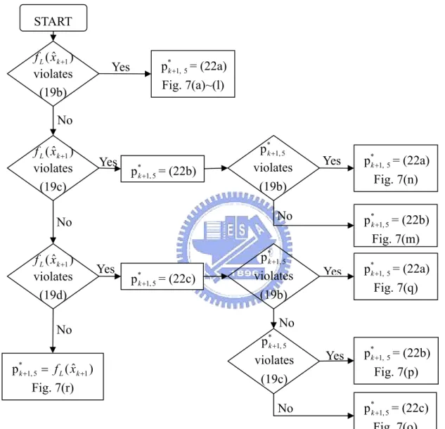
(9) List of Figures Figure 1.1. Flow chart of the system integration for the human-machine interactive motion. Figure 1.2. The motion control system for a six DOF motion simulator. Figure 2.1(a). Block diagram of the proposed ECAM system for mathematical representation. Figure 2.1(b). Block diagram of the proposed disturbance estimator for one practical embodiment. Figure 2.2. The estimation of external disturbance. Figure 2.3. The external disturbance estimator and external disturbance eliminated control. Figure 2.4. Temporal relations between the two proposed procedures. Figure 2.5. Cubic B-spline curve, rk +1, j (u ) , j = 1 to 4, and its control points, p k +1, 0 ~ p k +1, 6. Figure 2.6. Flow chart of the optimal solution process. Figure 2.7. The location of the optimal position command, p*k +1, 5 , for all different cases. Figure 2.8(a). Simulated angular velocity of the master. Figure 2.8(b). Simulated angular velocity of the master using disturbance estimator feedback control (zoom in). Figure 2.9. The errors between the fed torque ( τ L ) and the estimated torque ( τˆL ) with respect to various time constants ( ℑ ). Figure 2.10(a) The tracking error of the master’s position for the zero-order interpolation method Figure 2.10(b) The tracking error of the master for the third-order polynomial tracking method Figure 2.10(c) The tracking error of the master for the fourth-order polynomial tracking method Figure 2.10(d) The tracking error of the master for the fifth-order polynomial tracking method Figure 2.11. The piecewise tracking trajectory of the electronic cam motion; (a) the actual master’s position in real-time (b) the reference trajectory corresponding to the electronic cam motion (c) the actual cam trajectory in real-time. Note that the unit “counts” means the encoder’s pulse counts. The resolutions of the master’s encoder and the slave’s encoder are 2000 counts/revolution and 10000 counts/revolution, respectively. vii.

(10) Figure 2.12 (a) Cam profile error with the zero-order(conventional) tracking method (The maximum travel distance: 200000 encoder’s counts) Figure 2.12(b) Cam profile error with the third-order polynomial tracking method (The maximum travel distance: 200000 encoder’s counts) Figure 2.12(c) Cam profile error with the fourth-order polynomial tracking method (The maximum travel distance: 200000 encoder’s counts) Figure 2.12(d) Cam profile error with the fifth-order polynomial tracking method (The maximum travel distance: 200000 encoder’s counts) Figure 2.13(a) The tracking result of the slave velocity, acceleration and jerk purely based on the Lagrange polynomial curve-fitting with no optimization Figure 2.13(b) The result of the slave velocity, acceleration and jerk applying the optimization Figure 3.1. Classical linear washout filter (referred to Nahon and Reid, 1990). Figure 3.2. Block diagram of motion-cueing system, using the proposed control strategy. Figure 3.3(a). AWF structure (to be continued). Figure 3.3(b). AWF structure (to continue). Figure 3.4. Prototype SP-120. Figure 3.5. Kinematical skeleton of simulator platform SP-120. Figure 3.6. Restoration process in the dead zone washout filter. Figure 3.7. Washout trajectory along the i-axis, where the subscript i represents the three mutually orthogonal axes (x-, y-, and z-axis). Figure 3.8. Segmental data concerning linear accelerations along the x-axis. Figure 3.9. Segmental errors of linear accelerations along the x-axis, between the static scaled VR dynamic output ( a s , x ) and the simulator’s output ( a x ) using the (a) CLWF and (b) the proposed strategies. Figure 3.10. Three segmental data concerning Euler’s angular velocities. Figure 3.11. Segmental errors of Euler’s angular velocities between the static scaled VR dynamic output ( ω s, x ) and the simulator’s output ( ω x ) using (a) the CLWF and (b) the proposed strategies. Figure 3.12. Three segmental data concerning linear accelerations along the x-axis viii.

(11) Figure 3.13. Segmental errors of linear accelerations along the x-axis between the static scaled VR dynamic output ( a s , x ) and the simulator’s output ( a x ) using (a) the optimal pair of weighting parameters (1, 0) and (b) the pair of weighting parameters (1, 0.5). Figure 3.14. Three segmental data concerning Euler’s angular velocities. Figure 3.15. Segmental errors of Euler’s angular velocities between the static scaled VR dynamic output ( ω s, x ) and the simulator’s output ( ω x ) using (a) the optimal pair of weighting parameters (1, 0) and (b) the pair of weighting parameters (1, 0.5). Figure 4.1. Master switching method for q axes ECAM control. Figure 4.2. Cam profile trajectory established using the polynomial curve-fitting method. Figure 4.3. Cam profile trajectory established using the poly-line curve-fitting method. Figure 4.4. Conditions on dual solutions using the polynomial curve-fitting method. Figure 4.5. Equivalent model of slider. Figure 4.6. Simplified control system’s block diagram of control system of each slider of simulator SP-120. Figure 4.7. Upper. linear. fractional. transformation. with. ∆1 = δ m , ∆ 2 = δ c. and. | δ m | < 1, | δ c | < 1 Figure 4.8. Singular value frequency responses, σ (G1 ( jω )) , for various proportional gains, K a. Figure 4.9. Upper bounds of structured singular values, µ ∆ (G1 ( jω )) , for various proportional gains, K a. Figure 4.10. The piecewise ground earthquake signal involves only the translation. Figure 4.11. Power spectrum density of the ground earthquake signal at various frequencies. Figure 4.12. Comparison of Euler’s piecewise roll angle errors. Figure 4.13. Comparison of Euler’s piecewise pitch angle errors. Figure 4.14. Comparison of Euler’s piecewise yaw angle errors. Figure 5.1. Flow chart of the system integration of the human-machine interactive motion. Figure 5.2. Operating mode of the car dynamics ix.

(12) Figure 5.3. Colliding mode of the car dynamics. Figure 5.4. Hopping mode of the car dynamics. x.

(13) List of Tables. Table 2.1 An example of cam profile table, both sets of data are scaled by their largest travel distance of one cam cycle. Table 2.2. Experimental specifications of parameters for the ECAM control, last three data are scaled by their largest travel distance ( 40π rad) of one cam cycle.. Table 2.3. The maximum tracking error of the master’s position for the N th order polynomial tracking control (N = 0 ~ 5). Table 2.4. An experimental example for the maximum tracking errors of the slave’s position in the encoder’s counts for the N th order polynomial master tracking control, the maximum travel distance is 200000 encoder’s counts (equivalent to 40π rad). Table 2.5. An experimental example for the maximum slave velocity, acceleration and jerk based purely on the Lagrange polynomial curve-fitting and applying the optimization algorithm to the cubic B-spline curve-fitting process. Table 3.1. Capabilities of several motion simulators. Table 3.2. Comparison between the CLWF and the proposed washout filter in terms of the magnitudes of RMS ( E a ) , RMS ( Eω ) and PI using various static scaling factors ( s a , sω ), used successively to scale the linear accelerations and the angular velocities of VR dynamic output. Table 3.3. Magnitudes of RMS ( E a ) , RMS ( Eω ) and PI using various pairs of adaptive scaling factors ( λa , λω ); the static scaling factors ( s a , sω ) are set to (0.8, 0.7) (which will be later used to scale the linear accelerations and Euler’s angular velocities of VR dynamic output). Table 4.1. Maximum singular values of G1 ( jω ) ∞ , maximum structured singular values of sup µ ∆ (G1 ( jω )) and bandwidth of control system for various proportional gains, ω∈R. K a ; the upper bound, mH , of the nominal mass is set to 250 kg. Table 4.2. Critical upper bounds of the nominal mass for various proportional gains, K a. xi.

(14) Table 4.3. Root mean square (RMS) errors of Euler angles, obtained using the proposed master switching method and the conventional method for ECAM control Table executed on the simulator SP-120. xii.

(15) Nomenclature athreshold. = indifference threshold for acceleration. a. = acceleration received from the output of self-tuning process. ai. = the ith component of acceleration vector a. a AA. = specific acceleration of aircraft. aHP. = acceleration received from the output of high-pass filter. aHP , i. = the ith component of acceleration vector aHP. as. = acceleration obtained from scaling aVR. aref. = acceleration received from the output of dead zone washout filter. aref , i. = the ith component of acceleration vector aref. ares. = restoring acceleration in the dead zone washout filter. ares , i. = the ith component of acceleration vector ares. aVR. = acceleration obtained by summing gravity ( g I ) and applied force. aVR , i. = the ith component of acceleration vector aVR. a1 ( ) , a2 ( ). = acceleration function in adaptive washout filter. a2, i ( ). = the ith component of acceleration vector a2 ( ). Ec. = input voltage of the servo-motor. G. = mass center of the cockpit. g. = acceleration due to gravity. xiii.

(16) gI. = gravity vector in the inertia reference frame. HP filter. = high-pass filter. LP filter. = low-pass filter. L. = length of linkage. pi. = position of i th slider ball joint ( i = 1 to 6). qi. = position of i th ball joint (i = 1 to 6). O. qi. = coordinates of q i in the frame X-Y-Z-O. G. qi. = coordinates of q i in the frame x-y-z-G. Si. qi. = coordinates of q i in the frame x i - y i - z i - S i. Si. p i = Si [p xi p yi p zi ]T. = coordinates of p i in the frame x i - y i - z i - S i. O G. R (α , β , γ ). = rotational transformation matrix from x-y-z-G to X-Y-Z-O. Si O. R. = constant rotational transformation matrix from X-Y-Z-O to x i - y i - z i - S i (i = 1, 3, 5). RMS (•). = root mean square of •. s. = Laplace operator. sa. = static scaling factor used to scale the linear accelerations. sω. = static scaling factor used to scale the Euler angular velocities. sp. = lead screw pitch. (S to I). = transform from simulator to inertia reference frame. xiv.

(17) (S to J). = transformation of coordinates from x-y-z-G to x i - y i - z i - S i. TF. = transform from angular velocity to Euler angle rates. T. = system sampling time. u. = force applied to slider. X-Y-Z-O. = inertial coordinate system. O. = coordinates of G relative to the X-Y-Z-O frame. G. x-y-z-G. = cockpit coordinate system. x i - y i - z i - Si. = joint coordinate system (i = 1, 3, 5) used to represent the positions of slider ball joints pi and pi+1. ωindiff. = indifference threshold for angular speed. ω. = angular velocity received from the output of self-tuning process. ω AA. = specific angular velocity of aircraft. ωHP. = angular velocity received from the output of high-pass filter. ωs. = scaled Euler’s angular velocity ωVR. ωref. = angular velocity received from the output of adjustable scaling filter and yawing washout filter. ωVR. = Euler’s angular velocity. α. = roll angle of the platform (upper plate). β. = pitch angle of the platform (upper plate). xv.

(18) γ. = yaw angle of the platform (upper plate). φ = [α β γ ] = [φ x φ y φ z ] = Euler angle in the x-y-z-G frame. τ. = output torque of AC servo-motor. θ. = output angle of motor’s shaft. θ&. = angular velocity of motor’s shaft. xvi.

(19) Chapter 1 Introduction Recently, the applications of six degree-of-freedom (DOF) motion simulators have been widely developed, especially in flight simulation and vehicle simulation. The well-known examples are the ride films that generally use the motion identification method to perform the navigated motion. But there have been rarely developed for the human-machine interactive motion, especially in the simulators of small workspace. The main purpose of this dissertation is to study a motion control strategy to perform the human-machine interactive motion in a six DOF motion simulator. The system of human-machine interactive motion includes the following subsystems: cabin operating system, vehicle dynamics system, collision detection system, motion control system, sound effects and virtual reality system. Figure 1.1 shows the relations of these subsystems. This dissertation will be focused solely on the motion control scheme. As shown in Fig 1.2, the motion control system involves motion cuing control and trajectory tracking control in a six DOF motion simulator. Motion cuing control provides a strategy of motion trajectory generation such that the motion cue can be managed and displayed in a limited workspace. Another significant concern of a six DOF motion simulator is the trajectory tracking precision rather than the positioning accurate. This study proposes a novel trajectory tracking control algorithm to guarantee that the simulator’s motion always follows the trajectory of motion planning. In order to guarantee the correct motion cue, i.e.,. 1.

(20) the feeling of linear acceleration and angular velocity, a trajectory tracking control using the master-slaves control scheme based on the electronic cam (ECAM) tracking control structure is introduced in this dissertation. In this dissertation, chapter 2 presents an ECAM motion generation scheme with special reference to constrained velocity, acceleration and jerk; chapter 3 proposes a novel washout filter design for a six DOF motion simulator; chapter 4 uses the ECAM tracking control concepts, building a novel master switching method for ECAM control with special reference to multi-axis coordinated trajectory following; chapter 5 describes the system integration; chapter 6 concludes this dissertation. In this study, ECAM motion is generated in two stages, the first of which is a typical electronic gearing process which is focused on the velocity tracking control of the master motor. Steven [1] specified a tracking control electronic gearing system called an “optimal feed-forward tracking controller”, concerned primarily with the design of the slave controller. However, he did not consider the output properties of the master motor, including the measurement noise, periodic errors and external harmonic disturbances. In practice, the measurement noise or the external disturbance must be controlled and eliminated by modeling the disturbances, before applying tracking control to estimate the master position. This study proposes the used of a disturbance estimator [2] to suppress the external disturbance. The design of this disturbance estimator is practical and easy to implement.. 2.

(21) This approach to obtaining highly precise estimate of the master position involves N th order polynomial tracking. For example, the fifth order polynomial estimate is more precise than the third order polynomial estimate by a factor of about 10000. The advantage of the proposed tracking method is that the low-frequency harmonic disturbances of a loaded master are very precisely estimated. Such nominal harmonic disturbances are observed in many industrial applications [3]. In practice, the frequencies of the external disturbances are expected to be far below the Nyquist frequency [4] of the real-time system. ECAM motion regulates the slave motion to follow a predetermined trajectory, which is a function of the position of the master axis [5, 6]. A cam trajectory is generally specified by a cam profile table, which lists a set of reciprocal coordinates. Chen [7] applied B-spline [8, 9] and polynomial curve-fitting methods to generate a smooth cam profile curve function. Kim and Tsao [10] developed an electrohydraulic servo actuator for use in electronic cam motion generation, and obtained improved performance. However, some original performance limits, including velocity, acceleration or jerk constraints must be considered because motors have the lower loaded capacity relative to the hydraulic actuators. For example, for a highly precise machining tool, chattering must be avoided, so jerking in motion must be reduced. This study proposes an optimization algorithm [11] to prevent extremely high velocities, accelerations or jerks, yielding smooth motion of the slave motor without loss of precision. The proposed tracking method presented here was experimentally verified using a real-time. 3.

(22) program to realize the ECAM control system. The master’s system uses a disturbance estimator to eliminate external disturbances. This estimator is the prerequisite for the N th order polynomial tracking control. Lagrange polynomial [9] curve-fitting, cubic B-spline [9] interpolation and a constrained optimization algorithm are used to determine the position of the slaves. Consequently, a tradeoff may exist between precision and constraints, which are imposed in given order of priority. The purpose of the washout filter is to transform trajectories generated by a dynamic model of virtual reality (VR), which incorporates very large displacements, into driving system commands that can give a pilot realistic motion cues while remaining within the simulator’s limited workspace. Designing an efficient washout filter is a complex problem. These filters are first of all complex control systems whose robustness and stability must be ensured to prevent mechanical damage to the simulator. Furthermore, designs of washout filters must take into account the spatial-disorientation of the pilot making a “realistic” simulation hard to define. The problem’s complexity derives from human factors and the human-machine interaction. Many schemes have been presented in the last 20 years. Classical washout filters were developed first [12]-[14], followed by adaptive algorithms [15, 16], optimal control filters [17, 18], hybrid classical-adaptive filters [19] and robust filters [20, 21]. Importantly, even though these studies extensively address applications in simulators with relatively large workspaces,. 4.

(23) the performance of various techniques for simulating specific VR motion in a motion simulator with a restricted workspace has rarely been discussed. This study presents a novel washout filter design, that consists of a classical linear washout filter (CLWF), an adjustable scaling filter (ASF), a yawing washout filter (YWF), a dead zone washout filter (DZWF) and an adaptive washout filter (AWF). The CLWF separates the motion cues into high (“onset”) and low (“sustained”) frequency components so that cues can be managed and displayed within the physical confines of a given platform system. However, for motion simulators with severely restricted workspaces, even if the cutoff frequencies are properly selected [22], the position of cockpit may still exceed the platform’s workspace during a given motion because the linear accelerations and the angular velocities are mutually independent in the Cartesian coordinate system, but are coupled after applying inverse kinematics to every independent joint of the motion simulator. Moreover, the constraints on the driving system limit the performance of the motion simulator, such as the saturation for the driving current. Accordingly, the CLWF with appropriate cutoff frequencies is not always suitable for many practical platforms, especially those simulators with smaller workspace, but it remains useful in reducing the probability of leaving the limited workspace. The ASF dynamically tunes the cockpit’s angular velocities instead of the purely static scaling. Sometimes, the magnitude of linear acceleration is lower than the human sensible threshold [23]-[25], and the DZWF utilizes this moment to drive the cab stealthily back to its home. 5.

(24) position by accelerating it under the indifference threshold [23]-[25]. An AWF that includes the coordinate transformation from simulator to joints (S to J), washout function and self-tuning process, greatly improves the motive performance for strictly confined simulators. Two cost functions are defined to determine the performance index (PI) of VR motion. The PI quantifies the realism of the motion and is improved by inducing an empirical rule while adaptive scaling factors in the self-tuning process are tuned offline using numerical induction. Additionally, real-time software has been developed to implement the proposed criteria online in an automotive simulation for a six degree-of-freedom (DOF) motion simulator. Comparing the proposed washout filter with the CLWF shows that the experimental results indicate that the former is much more adaptive and realistic, especially for the motion simulator with a small workspace. The important issue of the robust stability of a six DOF motion simulator concerns its six axes cross-coupled behavior: each axis pulls and drags every other such that the most heavily loaded axis may act unexpectedly; that is, the actual trajectory of the cockpit may be unexpected. This phenomenon follows from inconsistent tracking of the planned trajectory and may cause the cockpit of the motion simulator to leave its nominal workspace. Thus, a trajectory tracking controller is urgently required. Numerous papers [26]-[28] exist around the parallel robots [29], which were focused on the dynamics analysis. Several articles have also referred to the design of controllers of a six DOF motion simulators. Chung, Chang and Lin. 6.

(25) [30] referred a fuzzy control system for a six DOF simulator and considered the hydraulic actuator system. Werner [31] introduced a robust tracking control for an unstable, linearized plant which was linearized. Plummer [32] described a nonlinear multi-variable controller for a flight simulator. The procedure for completely designing a robust controller of a nonlinear system consists of finding the nominal controlled plant [10, 33, 34, 35], which is very complicated and impractical; thus, the dynamics of the nonlinear control system must be linearized and simplified. Furthermore, to make motion planning of parallel robots, that are needed to calculate inverse and direct kinematical models. If the first one is often easy to solve, the second one is very complex for a six DOF parallel robot [36]. Usually, the selection is to make motion planning, either in joint space or in operational space [37]. This study introduces a master-slaves control strategy – master switching ECAM tracking control, based on the motion planning. The master switching ECAM control scheme presents a simplified control system for a six DOF motion simulator. ECAM tracking is applied to a multi-axes motion control system mainly to enable the slaves to follow consistently trajectories obtained from the predicted sets of reciprocal points of master and slaves. When the master receives a position command, it will or will not be driven to the desired position, and the slaves will be moved into new positions by following the predicted cam profiles. However, in a fixed master ECAM system, the heavily loaded slaves may follow a lightly loaded master, and then the slaves may lose tracking precision as. 7.

(26) it reaches its current (force) limit. Kim and Tsao [10] developed an electrohydraulic servo actuator for use in electronic cam motion generation, addressing the robust performance control for the fixed slave, an electrohydraulic servo actuator. Steven [1] specified an optimal feed-forward tracking controller, primarily associated with the fixed slave controller design. Each of their control schemes was demonstrated to satisfy the demands of precision and robustness, but to be valid only for its particular application. In the master switching control scheme, the most heavily loaded axis must be predetermined before anticipative motion begins: this axis will be treated as the master and the other axes as the slaves. The master may be switched between different types of motion from time to time, to exchange the master and one of the slaves in the subsequent action. After the master is instantaneously determined, the next important task is to build ECAM profiles from the demanded ECAM tables. Two curve-fitting methods [11] are proposed to establish piecewise ECAM profile. One is the polynomial curve-fitting method which is suggested for use in cases of low frequency motion. Simulations indicate that the polynomial curve-fitting method [9, 38] performs well, if the frequencies of the active body are less than one-tenth of half the system’s sampling frequency (Nyquist frequency). Restated, this method is favorable if and only if the trajectory of motion is very smooth from the viewpoint of the Nyquist frequency. The second method is the poly-line curve-fitting method, as shown in Fig. 3, which is more appropriate for higher frequency motion.. 8.

(27) A simplified dynamics model of the simulator for analysis is proposed to model the structured perturbation with parametric uncertainties. The well-known µ tool [39] is used to analyze the robust performance of the original control system, and then to demonstrate that it is more robust and stable after the proposed control scheme is applied to the system. Restated, real-time software was developed to implement the PC-based master switching ECAM control scheme used in the SP-120 motion simulator. Experimental results show the advantage of the proposed tracking accuracy. However, experimental analysis has also revealed that a shorter system sampling time yields more accurate tracking control, especially when the poly-line curve-fitting method is used. However, a tradeoff exists between the system sampling time and the calculation burden in a programming cycle.. 9.

(28) Chapter 2 Electronic Cam Motion Generation with Special Reference to Constrained Velocity, Acceleration and Jerk Electronic cam motion involves velocity tracking control of the master motor and trajectory generation of the slave motor. Special concerns such as the limits of the velocity, acceleration and jerk are beyond the considerations in the conventional electronic cam motion control. This study proposes the curve-fitting of a Lagrange polynomial to the cam profile, based on trajectory optimization by cubic B-spline interpolation. The proposed algorithms may yield a higher tracking precision than conventional master-slaves control method does, providing an optimization problem is concerned. The optimization problem contains three dynamic constraints including velocity, acceleration and jerk of the motor system.. 2.1 Prerequisite of Electronic Cam (ECAM) Tracking Control Electronic cam (ECAM) control is a well-known master-slaves system. Figure 2.1(a) schematically depicts a block diagram of the proposed ECAM control system for mathematical representation. The variables and symbols in the figure are defined in the following sections. In Fig. 2.1(a), the motion of the slave motor clearly depends on the estimated slave position command, p k +1 , which is generated by cubic B-spline interpolation, combined with an optimization algorithm. Such optimization is performed to meet the demands of limited performance - the constraints of velocity, acceleration and jerk. The method of cubic B-spline curve-fitting is based on substituting the estimated master position 10.

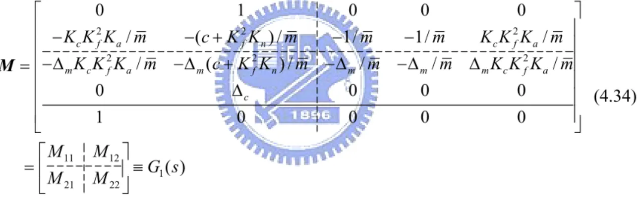
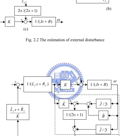
(29) into the cam trajectory. It is established using Lagrange’s interpolation formula to generate a Lagrange polynomial curve. However, the predicted master position is estimated by the electronic gearing (E-gearing) process. 2.1.1 External disturbance estimator External disturbances (or loads) applied to the master may directly impact the efficiency of E-gearing. Therefore, disturbances must be suppressed. A disturbance estimator, depicted in Fig. 2.1(a), is used to estimate and suppress the external loads of the master motor. However, Fig. 2.1(b) is one practical embodiment for the proposed disturbance suppressed control. In Fig. 2.1(b), the external load ( τ L ) is estimated from the input current ( ia ) and the angular velocity ( ω ), where K a , Lˆ f , Rˆ f , Kˆ , Jˆ and Bˆ represent the nominal back electromotive force constant, the nominal armature current inductance, the nominal armature current resistance, the nominal torque constant, the nominal moment of inertia and the nominal damping coefficient of the motor, respectively. Furthermore, Vref , L f , R f , K, J and B represent the reference voltage input, the actual armature current inductance, the actual armature current resistance, the actual (uncertain) torque constant, the actual (uncertain) moment of inertia and the actual (uncertain) damping coefficient of the motor, respectively. Consider the dynamics of a DC motor: Jˆω& + Bˆ ω + τ L = Kˆ ⋅ ia ⇒ τ L = Kˆ ⋅ ia − Jˆω& − Bˆ ω. (2.1) 11.

(30) According to Fig. 2.2(a), this estimator cannot be realized because of the differential term ( Jˆs ) of angular velocity. The estimator depicted in Fig. 2.2(a) is also very numerically sensitive to the measurement noise because it yields high gains in the high-frequency field. Accordingly, a first-order low pass filter is used to estimate the disturbance, τˆL , as shown in Fig. 2.2(b), where. τˆL =. 1 τL ( ℑs + 1). (2.2). and. τˆL − ( Jˆs + B ) Jˆ − Bˆ + Jˆ / ℑ = =− + ℑs + 1 ℑ ω ℑs + 1. (2.3). Rearranging this external disturbance estimator in Fig. 2.3 yields no differential term. The estimated disturbance ( τˆL ) is then fed back to the current loop, and the external disturbance is suppressed. In practice, due to the current-loop’s bandwidth is much larger than the speed-loop’s bandwidth, the electric dynamics ( 1 /( L f s + R f ) ) can be neglected in Fig. 2.1(b) for analysis. 2.1.2 Suppressing external disturbance According to Fig. 2.3, the pole of the disturbance estimator equals the pole of the low pass filter, specified by Eq. (2.2). Thus, the estimated value for low delay time is obtained by reducing the time constant ( ℑ ) of the low pass filter. However, the small time constant trades off the estimated precision and robustness because it suffers more on measurement noise and modeling uncertainty.. 12.

(31) Figure 2.2(b) is equivalently transformed to Fig. 2.2(c) to elucidate the effect of the external disturbance ( τ L ). According to Fig. 2.2(c), the effect of τ L is that of passing τ L through the filter ℑs /(ℑs + 1) . Accordingly, the external disturbance can be suppressed when the disturbance frequency is less than 1 / ℑ rad/s. Thus, the smaller time constant ℑ yields better efficiency for suppressing high-frequency disturbances. However, a trade-off exists between estimated precision and robustness, as described in the above paragraph. Due to considerations of robustness, the measurement noise and the modeling uncertainty must also be considered in determining the time constant ℑ . Appendix A discusses the sensitivities, S KGc , S JGc and S BGc to the uncertainties, where S KGc , S JGc and S BGc are the sensitivities of the current loop transfer function Gc to the uncertain parameters K , J and. B , respectively. Moreover, the effect of measurement noise is discussed with reference to a numerical simulation in Section 2.4.1.. 2.2 Electronic Gearing (E-Gearing) Process The electronic gearing (E-Gearing) differentiating itself from the mechanical gearing for that the E-Gearing system employed only electronic means to achieve the constant input/output velocity ratio. It is assumed that the output velocity control system is stiff and the main issue for the electronic gearing is to predict the future master velocity from its past. The velocity of the slave (output) motor is controlled according to the velocity of the master (input). 13.

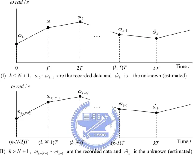
(32) motor. The velocity of the master motor varies when loads or other external disturbances are applied. Therefore, the master velocity is not usually constant and may exhibit harmonics. Even the amplitudes of the harmonic velocity are greatly reduced by using the proposed disturbance estimator, there still exists velocity variations. The procedure for estimating the master position and/or velocity is an important step for E-gearing. Methods of tracking control have been developed in various fields, and include radar tracking control [40] and others. This study proposes an N th order polynomial tracking method to perform the E-gearing process. According to the N th order polynomial, the master velocity at time t can be expressed as, N. ω = ∑ ci t i. (2.4). i =0. To determining the above coefficients ( c0 , c1 ,..., c N ) in real-time, two procedures are proposed. (I) Initial procedure, t = kT, 1 ≤ k ≤ N + 1 , is the various order ( ( k − 1) th order) polynomial extrapolation, where the symbol k is a real-time counter of time base, T is the PC-based programming sampling time and kT denotes the present time over all this dissertation. k −1. i ∑ ci (l ⋅ T ) = ω l , l = 0 to k-1. (2.5). i =0. Here use the assumption of 00 = 1 .. 14.

(33) (II) Main procedure, t = kT, k > N+1, is the fixed N th order polynomial extrapolation: N. i ∑ ci ( j ⋅ T ) = ω l , l = (k-N-1) to (k-1), j = l - (k-N-1). i =0. (2.6). Similarly, the symbol k is a real-time counter of time base, T is the PC-based programming sampling time. Where ω l ( = ( xl +1 − xl ) / T ) are the measured angular velocities during the interval [lT, (l+1)T], xl are the recorded positions of the master measured from the encoder at the past time lT. Furthermore, Figure 2.4 shows the temporal relations of the two proposed procedures. Rewriting Eq. (2.6) in matrix form yields,. Μ ⋅ Ck = Ω. (2.7). ⇒ C k = Μ −1 ⋅ Ω. where Μ ∈ R ( N +1)×( N +1) , C k ∈ R N +1 and Ω in this chapter are the obtained time matrix, the matrix of polynomial coefficients and the matrix of measured angular velocities, respectively. Moreover, the element of M in the i th row and j th column can be expressed as, m i , j = ((i − 1)T ) j −1. (2.8). C k = [c0 , c1 ,..., c N ]T , Ω = [ω k − N −1 , ω k − N ,..., ω k −1 ]T. (2.9). In Eq. (2.8), M is a constant matrix and Μ −1 exists; the computation involves no numerical degeneracy. Then the estimated velocity ωˆ k during the time interval [kT, (k+1)T] can be calculated as. ωˆ k = [1, NT ,...,( NT ) N ] ⋅ Ck. (2.10). 15.

(34) However, the estimated initial angular velocity may be chosen as the reference master velocity ( ω ) which is the desired velocity of the master, i.e. ωˆ 0 = ω . Then, the estimated position of the master is,. xˆ k +1 = x k + ωˆ k ⋅ T. (2.11). where xk and xˆ k +1 are the measured position of the master at the present sample time kT and the estimated position at the next sample time (k+1)T, respectively.. 2.3 Predicting the Position of Slaves This study uses Lagrange’s interpolation formula to establish piecewise cam trajectories. If the piecewise reciprocal master-slave’s coordinates, ( xi , yi ) , obtained from the given cam profile table, specify n+1 points, where i = 0 to n, and x0 < x1 < ... < x n , then the nth-degree Lagrange polynomial is, n. f L ( x ) = ∑ Li ( x ) yi. (2.12). i =0. where n. x − xj. j = 0, j ≠i. xi − x j. Li ( x ) = ∏ (. ). (2.13). are the Lagrange interpolation coefficients. Table 2.1 is an example of a cam profile table. Substituting Eq. (2.11) into Eq. (2.12), yields the next ideal cam profile position of the slave: n. f L ( xˆ k +1 ) = ∑ Li ( xˆ k +1 ) yi. (2.14). i =0. 16.

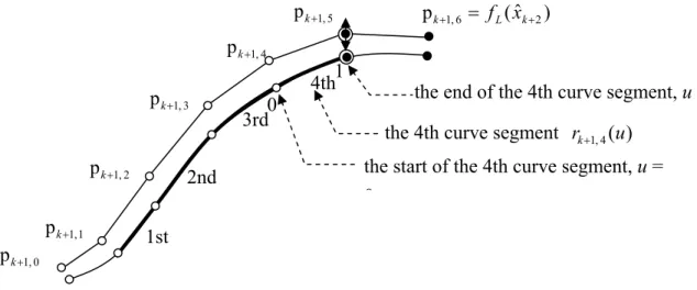
(35) However, in Eq. (2.14), as the order n increased, ripples and oscillations may occur [9]. Furthermore, the design of the cam profile may not consider the dynamic capability of the control plant in advance. Some dynamic limitations that degrade the slave motion generally apply; for example, a cutting machine tool may chatter due to over-large jerk, so the jerk has to be limited during the cutting process. Restated, maximal velocity and acceleration are limited by the motor and servo drive system. Consequently, the actual trajectory of slave motion may not be fulfilled Eq. (2.14), but must be close to the ideal trajectory provided fitting the specified constraints. Given its low sensitivity, the piecewise trajectory of the actual slave motion with respect to time is proposed to follow a cubic B-spline curve of fourth degree [9], as shown in Fig. 2.5: rk +1, j (u ) = F1, 4 (u ) p k +1, j −1 + F2, 4 (u ) p k +1, j + F3, 4 (u ) p k +1, j +1 + F4, 4 (u ) p k +1, j + 2 where rk +1, j (u ) represents the. j th segment of the ( k + 1) th time interval;. (2.15) j ∈ [1 : 4]. denotes the curve segment number and u = 0 to 1 within each curve segment. p k +1, j −1 ~ p k +1, j + 2 are the control points of the spline. F1, 4 (u ) ~ F4, 4 (u ) are the blending functions. The fourth degree cubic B-spline, as shown in Fig. 2.5, exhibits second-order continuity. All the variables of the B-spline are defined below. (I) p k +1, 0 ( = p k −4, 5 ) denotes the initial control point of the ( k + 1) th time interval, where p k −4, 5 is the previous position command of the slave at time (k-4)T and equivalently the fifth. 17.

(36) control point of the ( k − 4) th time interval. (II) p k +1, 1 ( = p k −3, 5 ) denotes the 1st control point of the ( k + 1) th time interval, where p k −3, 5 is the previous position command of the slave at time (k-3)T and equivalently the fifth control point of the ( k − 3) th time interval. (III) p k +1, 2 ( = p k −2, 5 ) denotes the 2nd control point of the ( k + 1) th time interval, where p k −2, 5 is the previous position of the slave at time (k-2)T and equivalently the fifth control point of the ( k − 2) th time interval. (IV) p k +1, 3 ( = p k −1, 5 ) denotes the 3rd control point of the ( k + 1) th time interval, where p k −1, 5 is the previous position of the slave at time (k-1)T and equivalently the fifth control point of the ( k − 1) th time interval. (V) p k +1, 4 ( = p k , 5 ) denotes the 4th control point of the ( k + 1) th time interval, where p k , 5 is the previous position of the slave at time kT and equivalently the fifth control point of the k th time interval. (VI) p k +1, 5 denotes the position command of the slave motor yet to be determined, and is equivalently the fifth control point of the ( k + 1) th time interval. (VII) p k +1, 6 ( = f L ( xˆ k + 2 )) denotes the sixth control point of the ( k + 1) th time interval, where f L ( xˆ k + 2 ) is derived from the cam profile position at time (k+2)T, as indicated in Eq. (2.14). Statements (I) ~ (VII) include a total of seven unknowns and six independent equalities. There is an extra degree of freedom left for the following optimization problem:. 18.

(37) The slave’s position error between the next unknown position command p k +1, 5 and the ideal cam profile position command f L ( xˆ k +1 ) at time (k+1)T can be expressed as, ek +1 = p k +1, 5 − f L ( xˆ k +1 ). (2.16). The objective error function is defined in quadratic form as, Ek +1 = ek +1. 2 2. = pk +1, 5 − f L ( xˆk +1 ). (2.17). 2 2. To ensure that the velocity, acceleration and jerk do not exceed the maximal values, ( Vmax , Amax and Jerk max ) allowed for the motor’s system, three inequality constraints are imposed on the optimization. The first-, second- and third-differentiation of the cubic B-spline curve at the start, u = 0, of the fourth segment, can be expressed as follows [9]. rku+1, 4 (0) = − 0.5p k +1, 3 + 0.5p k +1, 5. (2.18a). rkuu+1, 4 (0) = p k +1, 3 − 2 p k +1, 4 + p k +1, 5. (2.18b). rkuuu +1, 4 ( 0) = − p k +1, 3 + 3p k +1, 4 − 3p k +1, 5 + p k +1, 6. (2.18c). Minimizing the objective error function subject to the constraints on velocity, acceleration and jerk, yields the one dimensional constrained optimization problem: Minimize. subject to. p k +1, 5 − f L ( xˆk +1 ). 2. (2.19a). 2. | rku+1, 4 (0) | ≤ Vmax. (2.19b). | rkuu+1, 4 (0) | ≤ Amax. (2.19c). | rkuuu +1, 4 ( 0) |≤ Jerk max. (2.19d). The constrained optimization problem of a quadratic cost function has an easy-to-find 19.

(38) optimal solution,. p*k +1, 5 = f L ( xˆ k +1 ) with zero cost, when none of the constraints is violated.. According to equation (2.19a) ~ (2.19d), the optimization problem may be reformulated as an unconstrained minimization problem as follows: Minimize. 2. pk +1, 5 − f L ( xˆk +1 ) 2 + Wv g v (pk +1, 5 ) + Wa g a (p k +1, 5 ) + WJ g J (p k +1, 5 ). (2.20). where Wv , Wa and WJ are the weighting factors of velocity constraint, acceleration constraint and jerk constraint, respectively, and. ⎧⎪| | rku+1, 4 (0) | −Vmax |, if | rku+1, 4 (0) |< Vmax g v ( p k +1, 5 ) = ⎨ , if | rku+1, 4 (0) |≥ Vmax ⎪⎩0. (2.21a). ⎧⎪| | rkuu+1, 4 (0) | − Amax |, if | rkuu+1, 4 (0) |< Amax g a ( p k +1, 5 ) = ⎨ , if | rkuu+1,4 (0) |≥ Amax ⎪⎩0. (2.21b). ⎧⎪| | rku+1, 4 (0) | − Jerk max |, if | rkuuu +1, 4 ( 0) |< Jerk max g J ( p k +1, 5 ) = ⎨ , if | rkuuu ⎪⎩0 +1, 4 (0) |≥ Jerk max. (2.21c). In an extreme case that Wv >> Wa >> WJ , the minimization problem implies a constraint violation priority that g v is much more important than g a and g J . In practice, equation (2.19) is highly nonlinear, existing techniques to find the global optimization is not guaranteed. It needs to enumerate all the possible cases for the global solution. Figure 2.7 shows all the possible optimal solution for the extreme case that Wv >> Wa >> WJ . The bounds of p k +1, 5 for each of the constraints may be easily calculated from equations (2.19b), (2.19c) and (2.19d) by substituting the inequality sign into equality sign, as follows. p k +1, 5 = 2 ⋅ sign( rku+1, 4 (0)) ⋅ Vmax + p k +1,3. (2.22a). p k +1, 5 = sign( rkuu+1, 4 (0)) ⋅ Amax − p k +1,3 + 2p k +1,4. (2.22b). 20.

(39) 1 1 1 p k +1,3 + p k +1,4 + p k +1,6 p k +1, 5 = − sign( rkuuu +1, 4 ( 0)) ⋅ Jerk max − 3 3 3. (2.22c). The optimal solution process may be depicted in the flow chart as shown in Fig. 2.6. According to the flow chart, the solution of the optimization problem is unique, and thus guarantees to be the global optimum. In Fig. 2.6, all possible cases are enumerated and categorized as follows. (i) The ideal cam profile position command violates the velocity constraint, as shown in Figs. 2.7 (a) ~ (l); (ii) the ideal cam profile position command violates acceleration constraint and does not violate velocity constraint, as shown in Figs. 2.7(m) and 2.7(n); (iii) the ideal cam profile position command violates only the jerk constraint, as shown in Figs. 2.7(o) ~ (q); (iv) the ideal cam profile position command satisfies all of the constraints, as shown in Fig. 2.7(r).. 2.4 Simulation and Experimental Results 2.4.1 Simulation of disturbance estimator For simulation purposes, the nominal external disturbance is assumed to be a square wave function.. τL =. Amp. (2.23). The torque amplitude Amp of the square wave is set to 4.8773 ( N ⋅ m) and the frequency of the square wave is 1 Hz. Figures 2.8(a) and (b) present the master’s simulated angular velocity obtained using the proposed disturbance estimator feedback control and without. 21.

(40) using the disturbance estimator. The nominal parameters of the master motor defined in Section 2.1.1, are Kˆ = 0.55 ( N ⋅ m / A) , Jˆ = 0.093 ( kg ⋅ m 2 ) , Bˆ = 0.008 ( N ⋅ m ⋅ s / rad ) , L f = 0.046 H , R f = 1 Ω and K a = 0.55. V ⋅ s / rad . The sampling time of the current loop. is set to 0.001s in the simulation. Furthermore, the amplitude of the disturbance load torque is 4.8773 ( N ⋅ m) and the torque constant is 0.55 ( N ⋅ m / A) , that is, the operating current is 2. about 8.9 (A), the ia R f power loss is around 78.6 (W) (provided by the paper reviewer). However, the power loss of 78.6 (W) is not that serious for the applications with motors up to several kW. Figures 2.9(a) and (b) show the maximum errors between the fed torque ( τ L ) and the estimated torque ( τˆL ) for various time constants ( ℑ ). In Fig. 2.9(a), a smaller ℑ yields a smaller mean torque error. However Fig. 2.9(b) reveals that a lower ℑ yields a larger measurement noise. Furthermore, the measurement noise was assumed to be a zero-mean, normally (Gaussian) distributed random signal in the simulation. Both a larger mean torque error and a larger measurement noise reduce the tracking performance of the master, so the time constant must be neither too small nor too large. In the experiment, the time constant ( ℑ ) of the disturbance estimator was set to ten times the current loop sampling time. As depicted in Fig. 2.8(b), the time constant ( ℑ ) and the current loop sampling time are set to 0.01 sec and 0.001 sec, respectively. 2.4.2 Experimental results for tracking performance of the electronic gearing process. 22.

(41) Table 2.2 lists the parameter settings of the ECAM control. The accuracy of the tracking of the master’s velocity is characterized by the maximum error between the actual position and the estimated position. Figures 2.10(a) ~ 2.10(d) show that the maximum tracking error of the master’s position, using the fifth order polynomial tracking control method, is zero when the master’s nominal mean speed is 10π rad/s. Table 2.3 shows the maximum tracking error of the master’s position for polynomial tracking control methods of various orders (N = 0 to 5). 2.4.3 Performance of the electronic cam process Figure 2.11(b) shows an example of a reference trajectory that corresponds to the electronic cam motion. According to a constant master speed of 10π rad/s and a maximum slave travel distance of 40π rad, the reference trajectory yields a 100π rad/s maximum slave speed, 630π rad / s 2 maximum acceleration and 4060π. rad / s 3 maximum jerk.. The master’s speed is generally not constant and may be harmonic, as shown in Figs. 2.8(a) and (b). The speed will exhibit the actual position of the master and the ideal cam trajectory, as shown in Figs. 2.11(a) and 2.11(c), respectively. This piecewise cam trajectory contains 191 points. Three performance indices are used to quantify the accuracy and consistency. The tracking accuracy of the slave motion is characterized by the maximum error and the root mean square (RMS) error. The consistency of the cam tracking – that is, the cycle-to-cycle variation - is characterized by the RMS difference between the particular error response and. 23.

(42) the error response averaged over a number of cycles. Fifty cycles of tracking error data were collected. Figures 2.12(a) ~ 2.12(d) summarize the results of slave position. Table 2.4 lists the maximum tracking errors of the slave’s position in encoder counts, using the N th order polynomial tracking control method and the pure Lagrange polynomial curve-fitting method. Furthermore, Fig. 2.13 shows the partial results of the slave’s tracking velocity, acceleration and jerk, according to Lagrange polynomial curve-fitting with or without the aforementioned optimization. Similarly, Table 2.5 indicates the tracking control performance, also for the Lagrange polynomial curve-fitting method with or without the aforementioned optimization. 2.4.4 Computational load on the CPU of the proposed ECAM tracking control The selection of N depends on the accuracy demanded. As stated above, tracking using a higher order polynomial yields higher precision; however a tradeoff exists between the “order” of the polynomial used and the CPU time required. In practice, the computational time of the proposed algorithm (fifth-order tracking) is about 0.02 ms in a programming cycle on an Intel Pentium III 900MHz CPU. The computational time of a programming cycle is much less than the PC-based sampling time, 10 ms.. 24.

(43) Chap 3 A Novel Washout Filter Design for a Six Degree-of-Freedom Motion Simulator The motion cue performed by a motion simulator is restrained by the workspace of the simulator structure. A typical reasoning is then to build a large motion simulator unless it is for entertainment, which involves in small simulators. This study proposes a novel approach to designing the washout filter of the motion control of a six degree-of-freedom motion simulator for entertainment purposes. Using information obtained from the inverse kinematics of the simulator, the workspace boundary, detected in real-time, is fed into the washout filter as a reference for the motion planning. The main focus of this approach is to make the motion cue feasible for use in a simulator with a restricted workspace, while ensuring the robustness of the driving system. In this paper, different indices are established to specify the performance of the motion cue. A classical linear washout filter was implemented and compared with the proposed washout filter using the performance indices to demonstrate the benefits of the latter.. 3.1 Inverse Kinematics The motion cue control may be also called the cockpit position control, because the position of the cockpit, including both translation and rotation, must be transformed into the coordinates of the six sliders’ ball joints (S to J) using inverse kinematics. The inverse kinematics of the motion simulator SP-120 (Fig. 3.4) is presented as follows. As shown in Fig. 3.5, the coordinate of. Si. p i = Si [p xi p yi p zi ]T is determined by. 25.

(44) || Si q i − Si p i ||2 = L2. (3.1). in which all parameters are fixed in the Si coordinate system, where Si. and. O G. q i = Si O+ SiO R ⋅ [ O G + GO R (α , β , γ )⋅G q i ]. (3.2). R (α , β , γ ) is the transformation matrix of the Euler angle and can be expressed as,. cβcγ ⎡ ⎢ O G R (α , β , γ ) = ⎢ sαsβ cγ + cαsγ ⎢⎣- cαsβ cγ + sαsγ. - cβ sγ - sαsβsγ + cαcγ cαsβsγ + sαcγ. sβ ⎤ - sαcβ ⎥⎥ cαcβ ⎥⎦. (3.3). and cβ = cos β , sα = sin α ,…. and so on.. 3.2 Preview of Classical Linear Washout Filter (CLWF) The most widely used CLWF drive rules today are derived from the design of Schmidt and Conrad [13]. Figure 3.1 shows a block diagram of the typical implementation [14]. Modern implementations tend to drive the simulation with angular rates rather than angular accelerations, since this method has generally been found to produce a more realistic cue. As shown in Fig. 3.1, specific acceleration ( a AA ) is transformed to the inertial reference frame (S to I) and converted into acceleration ( aVR ), obtained by summing gravity ( g I ) and applied forces before the high-pass filter operation is performed. This approach uses a more convenient frame of reference for generating the commands of the simulator’s driving system. Similarly, high-pass onset filtering is applied to the scaled Euler’s angular velocity ( ω s ). The low-frequency specific acceleration components are low-pass filtered, and operated upon by a. 26.

(45) "tilt coordinate" block, much like that in Schmidt and Conrad's residue-tilt design; the tilt coordinate cross-feed is rate-limited to ensure that the commanded rates do not exceed the pilot's indifference threshold, which is set to 3 deg/s [23]. As stated above, the CLWF technique is combined with the following auxiliary washout filters, yielding a novel washout filter, presented in Fig. 3.2.. 3.3 Adjustable Scaling Filter (ASF) and Yawing Washout Filter (YWF) The limited workspace of the simulator constrains the Euler angles, including roll, pitch and yaw. Therefore, this paper proposes that the angular velocity of the cockpit must be adjusted by a dynamic tuning process called adjustable scaling filtering which involves a nonlinear filter, rather than by purely static scaling down, which would also reduce the active intensity even if the angular rates are originally lower. Applying this nonlinear filter can guarantee that the signals of angular velocities, fed to the simulator are more realistic than those associated with traditional static scaling down, unless the limited workspace is sufficiently large that the magnitude of the static scaling factor is approximately unity. Restated, the degree of scaling down is traded off with the limited size of the workspace, but can be greatly reduced after the ASF is used. The algorithm is as follows.. φ i ,k +1 = φ HP ,i ,k +1 , if || (φ HP ,k +1 ) ||2 ≤ φ critical φi ,k +1 = φi ,k +1 ⋅ φcritical / || φHP ,k +1 ||2 , if || (φ HP ,k +1 ) ||2 > φ critical. 27. (3.4).

(46) and,. ω i ,k = (φ i ,k +1 − φ i ,k ) / tVR. (3.5). where φ i,k and φ HP ,i ,k both represent the present Euler angles, the latter of which is received from the high-pass filter at time ktVR ; φ critical is the magnitude of a given critical Euler angle; •. 2. represents the 2-norm of • ; tVR is the sampling period of VR; both ω i ,k and. ω HP ,i ,k are present Euler angular velocities, the latter of which is received from the output of the high-pass filter at time ktVR . The subscript i indicates the i-axis (i = x, y or z). Applying the above algorithm greatly improves the rotational performance of the motion simulator, not only to prevent the cockpit from moving outside the limited workspace during pure rotation but also to obtain more realistic angular velocities or attitudes of the platform during real-time VR motion. Importantly, the platform’s attitude in terms of roll and pitch involves an actual tilt coordination that enables the pilot to feel the component of gravity; thus, the roll or pitch cannot be arbitrarily changed during the restoration unless the attitude is obtained by low-pass filtering of the acceleration along the y- or x-axis, as in residue tilt. Contrarily, the yaw angle is not important: the only concern is the yawing velocity. Therefore, a yawing washout algorithm is proposed as follows. if (φz ,k +1 < φz ,critical and ωHP,z,k > ωindiff ) or sign(ωHP,z,k ) = − sign(φz,k ) ⇒ ω z ,k = ω HP , z ,k ,. (3.6). 28.

(47) if ( φz ,k +1 ≥ φz ,critical or ωHP,z,k < ωindiff ) and sign(ω HP,z,k ) = sign(φ z,k ) , and t ≤ t res , yaw ⇒ ω z ,k = − sign(φ z ,k ) ⋅ ω indiff. (3.7). where φ z,critical is the given critical yaw about the simulator; ω indiff is the indifference threshold for angular speed; t and t res, yaw are the present restoring time and the total periodic restoring time, respectively, and. t res , yaw = | φ z ,k | / ω indiff ,. (3.8). where, ⎧ sign(•) = 1, if (•) > 0 ⎪ sign(•) = -1, if (•) < 0 ⎨ ⎪⎩ sign(•) = 0, if (•) = 0. Applying the above yawing washout algorithm, the zero-crossing phenomenon does not occur during the yawing washout period, facilitating the other actions including roll, pitch and translation.. 3.4 Dead Zone Washout Filter (DZWF) During the restoration period, the limitations on linear acceleration and angular velocity [24, 25] almost prohibit the restoration of the cockpit to its home position except by extending the restoration period, or when the original motion in VR are at sufficiently low frequencies. Clearly, extending the restoration time may cause some significant motion to be lost, so this strategy is not favored. Translation with lower frequencies may give enough time to carry the cockpit back stealthily after proper high-pass filtering is performed, but generally, such a 29.

(48) motion implies unexcited motion and poorly represents most normal actions. Consequently, a proposed strategy, called dead zone washout filtering, is adept at utilizing time. Dead time is defined as the period during which the linear acceleration is lower than the pilot’s sensible threshold [23]-[25]. Restated, the acceleration enters the dead area during this dead time; otherwise, it is in the scaled area. During the dead time, the cockpit is translated to its home position rather than being scaled to zero. Every component of the restoring acceleration ares ∈ R 3 must be lower than the indifference threshold a threshold (0.17~0.28 m / s 2 [25], here set to 0.017g). Even if the restoring acceleration slightly exceeds the indifference threshold, an adaptive restoring acceleration must be modified as follows, to prevent the workspace boundary from being touched. ⎧| a res , i |= v 0, i 2 / 2 S max, i , if | v 0, i | ≥ 2a threshold S max, i ⎪ ⎨ ⎪⎩| a res , i |= a threshold , if | v 0, i | < 2a threshold S max, i. (3.9). where S max, i is the maximum distance from the present position to the nominal workspace boundary in the direction of the present velocity v0, i ; subscript i indicates the i-axis (i = x, y or z). The next urgent task is to determine the maximum restoration period. Figure 3.6(a) indicates a situation in which the present velocity has the same direction as the present displacement, with reference to the home position. Figure 3.6(b) presents a situation in which the present velocity is in the opposite direction from the displacement. These two cases are 30.

(49) both treated by the basic law of kinematics, yielding,. t1 = sign( Pcur , i ) ⋅ v 0, i / | a res , i | + (1/2) 2v 0, i 2 / a res , i 2 + 4d i / | a res , i |. (3.10). t 2 = sign( Pcur , i ) ⋅ v 0, i / | a res , i | + 2v 0, i 2 / a res , i 2 + 4d i / | a res , i |. (3.11). d i = | Phom e, i − Pcur , i |. (3.12). and,. where d i is the distance from the present position to the home position along the i-axis; Phom e, i and Pcur , i are the home position and the present position along the i-axis, respectively; t1 is the period of deceleration and t2 is the total restoration period. The velocity is importantly guaranteed to be zero at the restoring time t 2 . During the restoration period, the restoring action will continue unless the direction of acceleration along the i-axis is opposite neither that of the present velocity nor the present position. Then, the active acceleration along the i-axis can be expressed as, ⎧⎪ ai = aHP , i , if aHP , i > athreshold and sign(aHP , i ) = − sign( vcur , i ) = − sign( Pcur , i ) ⎨ ⎪⎩ ai = ares , i , others. (3.13). where a HP , i represents the linear acceleration along the i-axis, received from the output of high-pass filter, and vcur , i is the present linear velocity along the i-axis. Like the yawing washout, the DZWF procedure involves no zero-crossing and improves the rotational performance. Restated, it greatly reduces the cross coupling of rotation and translation.. 31.

(50) 3.5 Structure of the Adaptive Washout Filter (AWF) This DZWF algorithm cannot always guarantee that the cockpit of simulator does not leave the actual workspace because not all of the workspace boundaries are very explicit. Therefore, adding an adaptive washout filter is proposed to compensate for the insufficiency of the prior proposed filters and thus accommodate the more severe restrictions, such as the smaller workspace and the limited driving current. The AWF involves the transformation (S to J), the washout function (Fig. 3.3(a)) and the self-tuning process (Fig. 3.3(b)). 3.5.1 Transformation (S to J) The transformation (S to J) is presented using inverse kinematics, as described in section 3.1. 3.5.2 Washout Function The purpose of the washout function (Fig. 3.3(a)) is to prevent the cockpit from exiting its limited workspace. Figure 3.7 depicts a trajectory along the i-axis proposed to plan the washout motion, initially making the pilot feel an instantaneous linear acceleration and later carrying the cockpit to its starting position stealthily in the period t d ≤ t ≤ t f . The planned trajectory is as follows. The continuous trajectory P(t) ∈ R 3 of the translation of the cockpit consists of two cubic polynomial segments.. P(t) = P1 (t ) + P2 (t ). for. 0≤ t ≤ tf. (3.14). 32.

(51) where the vectors P1 (t ) and P2 (t ) are in R 3 ; P1 (t ) = 0. for t d ≤ t and. P2 (t ) = 0. for t < t d. The P(t) at t f is the desired target position and that at t d is the transition position. At least eight constraints on P(t) are evident. The initial and final values of the function are constrained.. P(0) = 0, P( t f ) = 0. Continuity at the transition position yields,. P1( t d -) = P2( t d +). The function yields continuous velocities, implying that the initial and transitional velocities’ vectors ( R 3 ) are both continuous and the final velocity’s vector is zero in the procedure of washout motion planning, and can be expressed as,. v(0) = v0 , v( t f ) = 0, v1( t d -) = v2( t d +). A further constraint is that the transition acceleration must be continuous:. a1( t d -) = a2( t d +) ∈ R 3 . The following equation implies that the initial acceleration must fulfill the demands of VR – to ensure that the pilot feels an instantaneous linear acceleration. a1 (0) = aref ∈ R 3. where aref is the linear acceleration received from the output of the DZWF. These eight. 33.

(52) constraints can be used to determine two consecutive cubic polynomial segments, since two such segments have exactly eight coefficient vectors.. P1(t) = b0 + b1t + b 2t 2 + b3t 3. (3.15). P2(t) = c 0 + c1t + c 2t 2 + c 3t 3. (3.16). where the eight vectors, b0 , b1 , b 2 , b3 , c 0 , c1 , c 2 , and c 3 are all in R 3 . The vectors of velocities and accelerations along the path are derived as follows.. v1 (t ) = P&1 (t ) = b1 + 2b 2t + 3b3t 2. (3.17). v2 (t ) = P&2 (t ) = c1 + 2c 2t + 3c 3t 2. (3.18). a1 (t ) = P&&1 (t ) = 2b 2 + 6b3t. (3.19). a2 (t ) = P&&2 (t ) = 2c 2 + 6c 3t. (3.20). Combining Eqs. (3.15) to (3.20) with the eight constraints yields eight-by-three constrained equations in eight-by-three unknowns. Let t d = κt f , where 0 < κ < 1 . Now,. b 0 =0. (3.21). b1 = v0. (3.22). b 2 = aref / 2. (3.23). b3 = (2 aref κ t f +2 v0 κ+ aref t f +4 v0 ) / (6 κ t 2f ). (3.24). c 0 = -κ2 t f ( aref t f +4 v0 ) / (6 (1 − κ ) 2 ). (3.25). c1 = (2 v0 (1+ κ 2 )+ aref κ t f ) / (2 (1 − κ ) 2 ). (3.26). c 2 = ( aref κ 2 t f -4 v0 -2 aref κ t f ) / (2 t f (1 − κ ) 2 ). (3.27). 34.

(53) c 3 = (- aref κ t f (3-2κ)-2 v0 (3- κ 2 )) / (6 (1 − κ ) 2 t 2f ). (3.28). From Eq. (3.20), the maximum linear deceleration is a2 (t d ) , and, a 2,i (t d ) ≤ a threshold. (3.29). where the subscript i represents the three mutually orthogonal axes (x-, y-, and z-axis), and a2,i (td ) is the component of a2 (t d ) along the i-axis. Equation (3.28) implies that κ can be treated as a ratio to constrain deceleration during the restoration. The magnitude of deceleration must be constrained below an indifference threshold athreshold to prevent the pilot from becoming aware of this restoration [25]. The maximum displacement is at a stationary value when the velocity is zero. For the second segment of the polynomial,. v2(t) = c1 + 2c 2t + 3c 3t 2 = 0 which yields, t 2, PMAX = t f (2 v 0, i (1+κ 2 )+ a ref , i κ t f ) / (2 v 0, i (3-κ 2 )+ a ref , i κ t f (3-2κ)) > td. (3.30). The maximum displacement along the i-axis is obtained by substituting t 2, PMAX into the i-axis washout function Pi (t ) , such that, PMAX , i = Pi (t 2,PMAX ). (3.31). which will be used to determine whether the washout planning is executed. 3.5.3 Self-Tuning Process (Fig. 3.3(b)) The saturation of the driving current also constrains the performance of the simulator,. 35.

(54) and may cause the angular speed of the servo motor to exceed its critical value and, causing a problem related to the robustness of the driving system. Additionally, motion may sometimes still violate the workspace after filtering, because the indifference threshold of deceleration always limits the washout efficiency. Thus, a final check on the self-tuning process is proposed to guarantee that the system of motion simulator is robust. The following steps determine the rules. 1. Calculate whether the commanded velocity fed to the driving system exceed the critical value. 2. Calculate whether the cockpit will be outside the limited workspace. 3. If at least one of the answers to the preceding questions is positive, let the linear acceleration and the angular velocity be multiplied by two appropriately predetermined scaling functions, p a ( λa ) and pω ( λω ) , respectively. Then, redo steps 1 and 2 until the answers are both negative or the iterative loop is performed more than n times, where n is the number limit in this chapter preset by considering whether the total calculation time will meet the demands of real-time programming. The following two simple equations represent the above strategies. a = aref ⋅ pan ( λa ) and ω = ωref ⋅ pωn ( λω ). (3.32). where a ∈ R 3 and ω ∈ R 3 represent the cockpit’s present linear acceleration and angular velocity, respectively; aref and ωref (Fig. 3.2) are the linear acceleration received from the. 36.

(55) output of DZWF and the angular velocity that combines the output of ASF with the tilt coordination, respectively. The functions p a ( λa ) and pω ( λω ) are the adaptive scaling functions of linear acceleration and angular velocity, respectively. The adaptive scaling factors. λa and λω are properly predicted before the first simulation test and are later tuned offline by inducing an empirical rule to obtain a heuristically selected pair of adaptive scaling factors, as described in the next section.. 3.6 Performance Index In this paper, the VR motion fed to the specific motion simulator-SP120 is specified by a performance index (PI) combined with two cost functions, E a ,k and Eω ,k . E a ,k = [ a( ktVR ) − aref ( ktVR ) / RMS ( aref )] ⋅ RMS ( aVR ) / RMS ( aref ) 2. = RMS ( aVR ) ⋅ (1 − p ( λa )) aref ( ktVR ) 2 /[ RMS ( aref )]2 nk a. 2 2 Eω ,k = [ ω2 ( ktVR ) − ωref ( ktVR ) / RMS ( ωref )] ⋅ RMS ( ωVR ) / RMS ( ωref ) 2. 2 2 = RMS ( ωVR ) ⋅ (1 − pω (λω )) ωref ( ktVR ) /[ RMS ( ωref ) ⋅ RMS ( ωref )] 2 nk. (3.33). (3.34). 2. and, PI = Wa ⋅ RMS ( E a ) + Wω ⋅ RMS ( Eω ) N. (3.35) N. 2. 2. RMS ( E a ) = ( ∑ E a ,k ) / N , RMS ( Eω ) = ( ∑ Eω ,k ) / N k =0. where Wa and Wω. k =0. (3.36). are the weighting parameters of RMS ( E a ) and RMS ( Eω ) ,. respectively; RMS (•) means the root mean square of • ; N is the total number of samples of VR motion; n k is the total number of self-tuning iterations at time ktVR and is. 37.