政府支出之生產與最適公債比例 - 政大學術集成

全文

(1)國立政治大學社會科學院經濟學系碩士論文 Department of Economics College of Social Sciences National Chengchi University Master Thesis. 政府支出之生產與最適公債比例治. 立. 政. 大. ‧ 國. 學. Government Expenditure in Production and. Nat. 莊仲霖. er. io. sit. y. ‧. the Optimal Debt Ratio. n. a l Chuang, Chung-Lin i v n Ch U engchi 指導教授: 黃俞寧博士. Advisor: Hwang, Yu-Ning, Ph.D.. 中華民國 101 年六月 June, 2012 I.

(2) 謝辭. 夏季的蟬鳴，傾訴著這近一年來的辛勞，儘管微不足道，但老師的認真讓人無法忘掉。還記得寒假之前，常常沒有約好下去打擾老師，但感謝老師依舊細心糾正我的問題。一篇論文的誕生，或許不難；但一份關係的建立，絕對不簡單，也就在這種關係下，漸漸的讓我開始懂得去思考。對老師的感激，無法言表。感謝口委張淑華教授，張瑞娟老師，老師們細心的指導讓我得以全盤檢視自己的問題，並重新看待自己的作品。然而，即使如此，時至此刻，我依舊無法相信自己可以完成。在這段過程中點點滴滴，感謝十四樓的各位，感謝班上的同學，感謝各位曾經用心對待過我的人，更感謝我的好友承穎，長時間的借我筆電讓我得以完成。另外，也十分對不起那些一直在聽我抱怨的人，塞了許多垃圾在你們耳中，在此表達歉意。在完成一份作品當時，瞬間的感動也遲遲讓人無法冷靜下來，而這份感動也就來自於那些曾經在這段時間內幫助過我的人，即使這段過程中並非十分美好，但畢竟，痛苦會過去，美好會留下，所講的也或許是這意思吧！而如今，那曾經無法出去的我也走到了這一步，這一切都要感謝我的父母，感謝爸爸，媽媽，我以身為你的兒子為榮，也在此將自己拙作送給你們。. 立. 政治大. ‧. ‧ 國. 學. n. er. io. sit. y. Nat. al. Ch. engchi. II. i n U. v 民國一百零一年六月莊仲霖.

(3) 中文摘要. 2011 年，美國政府在經歷次級房貸和高軍事支出的雙重壓力下，爆發高度財政赤字的問題，造成歐巴馬政府面臨調高債務比例與債務上限的壓力。然而，在眾多的輿論聲中，美國民主黨與共和黨在八月底達成下列協議，減少政府支出、提高債務比例以及增加債務上限等；但是，是否這些方式將改善美國經濟？本篇文. 政治大加入私人廠商部門，透過公共投資，幫助私人廠商增加產出；並且在政府僅採行立. 章在動態隨機一般均衡(DSGE)架構下，建立一個封閉經濟體系，並將政府支出. 公債和徵稅融通下，找出一個最適的債務持有比例，使國內福利為最高。而本文. ‧ 國. 學. 發現政府進入生產部門時，將影響最適債務持有比例。即是，隨著政府支出生產. ‧. 彈性越大，最適債務持有比例也會上升，而在基準參數下，我們將會得到最適債. er. io. sit. y. Nat. 務持有比例為百分之十的結論。. al. n. v i n 政府支出、動態隨機一般均衡(DSGE)、政府支出生產彈性、 Ch engchi U. 關鍵字：. 最適債務持有比例. III.

(4) Abstract. In 2011, under the pressure of subprime mortgage and high military expenditure, the U.S. government accumulated high fiscal deficit, and the Obama government faced the pressure of raising debt ratio and raising debt ceiling. However, among the huge debates, the Republican Party and Democratic Party reached the deal in August which included cut-down government expenditure, raise debt ratio, raise debt ceiling, and so on. But, will these ways improve the U.S. economy? This paper follows the dynamic. 政治大 which the government helps 立private firm to production through public investment. stochastic general equilibrium (DSGE) framework to construct a closed economy,. ‧ 國. 學. Besides, given that government only undertakes debt financing and tax financing, we try to find an optimal debt ratio which makes the highest domestic welfare. In our. ‧. finding, if the government enters private production sector, the optimal debt ratio will. sit. y. Nat. be influenced. That is, the optimal debt ratio will increase with the production. n. al. er. io. elasticity of government expenditure. Under the benchmark parameter, the optimal debt ratio is 10 percent.. Ch. engchi. i n U. v. Key Word: government expenditure, DSGE, production elasticity of government expenditure, optimal debt ratio. IV.

(5) Contents. 1. Introduction……………………………………………………………..………1 1.1 Motivation……………………………………………………………..……1 1.2 Literature review………………………………………………….…….…..5 2. The model……………………………………………………………….……….9 2.1 The household……………………………………….…………….…….…9 2.2 The Firm……..…………………………………………………………….11. 政治大 2.4 Central bank……..……………………………………………….….…..…13 立. 2.3 Government……………………………………………………….……….12. 2.5 Market clearing condition…………..…..……………..………….………..13. ‧ 國. 學. 3. Steady state and Calibration……………..……………..……………….……….14. ‧. 3.1 The all steady state equations……………..……………..……………..….14. sit. y. Nat. 3.2 Solve the endogenous variable under steady state…………………….…..14. io. er. 3.3 Structure parameter and calibration……………..……………………...…15 3.3.1 Steady state analysis……………..……………..………………………17. al. n. v i n C h government productivity………….….…..17 3.3.2 Steady state under different engchi U. 3.3.3 The steady states under different debt to GDP ratios……………….….18. 4. Dynamics……………..……………..……………..……………..………..…....18 4.1 Productivity shock……………. ……………..……………..……….……..18 4.2 Sensitivity analysis…………………………………...………………..…...20 5. Welfare measure……………………………………….…………………...…...23 5.1 The welfare criterion……………..……………………………..…….…….23 5.2 Welfare analysis of optimal policy………………….…………..…….……24 5.3 The optimal policy under different government productivity….…….….…24 6. Conclusion……………………………..…………….……………..………..…26 V.

(6) Reference……………..……………..……………..……………..……………….27 Appendix……………..……………..……………..……………..……………….30. 立. 政治大. ‧. ‧ 國. 學. n. er. io. sit. y. Nat. al. Ch. engchi. VI. i n U. v.

(7) 1. Introduction. 1.1Motivation. In the 21th century, the United States has been facing a dramatic change in economic development and national defense. George W. Bush continued to take expansionary fiscal policy on military expansions and took tax cut as dispatching army to Iraq. All of those made the U.S. government’s budgetary deficit rose widely.. 政治大 economic recession and made the U.S. fiscal status to face crisis. The overall U.S. 立. Furthermore, the subprime mortgage crisis burst in 2008, which exacerbated. debt increased almost 2.6 trillion dollar during Bush government period and the debt. ‧ 國. 學. to GDP ratio increased to almost 30 percent. 1 The huge debt made the Obama. ‧. government to increase the debt ratio, raise the debt ceiling, and cut down the. sit. y. Nat. government expenditure. Hence, the U.S. faces a serious debt crisis, which influenced. io. 2013.2. al. er. the reputation of the U.S., and the U.S. debt ratio is predicted to exceed 100% in. n. v i n C hthe debt and reduce Is it a good policy to increase the expenditure? Although engchi U. someone who argued it is good, still someone disagreed. Krugman (2010) suggests that the U.S. government should increase expenditure to stimulate economy growth.3. Hence, the debate arouse our interests in government expenditure influence the U.S. 1. After the Bush government, the Obama government expected that economy can recover by taking quantitative easing monetary policy and selling public debt, and budget can be balanced through economic growth. Unfortunately, what the Obama government did had made fiscal deficit more serious and higher inflation. Then, with the debt maturity dating coming, what the Obama government can do is to just adjust the debt ceiling under the default crisis 2 In 2011 Obama government reached an agreement in the congress. This is, raise the debt ceiling gradually to pay the great debt, reduce government expenditure, and extend the tax cut policy from Bush government time to 2013. But there are existed many argue about the deal. Some economist favor that government reduce the spending debt to GDP ratio. 3 Krugman (2010) in his written ‘’Bad Analysis At The Deficit Commission’’ said that the growth slowly not because the debt(Reinhart and Rogoff, 2010) accumulate but the war. Link: http://krugman.blogs.nytimes.com/2010/05/27/bad-analysis-at-the-deficit-commission/ 1.

(8) economy. Arrow and Kurz (1970), who added the government expenditure to production function first. After that, Ratner (1983) estimated a production function, in which private output is dependent variable, and independent variables include employment, private capital, and government expenditure. Aschauer (1988) also estimated the same equation by the ordinary least squares method, and pointed out the nonmilitary government expenditure, including streets, airports, electricing, highways, gas facilities, water systems, and sewers are more productive to private production. We can see the same way as Fisher and Turnovsky (1998), and Barro (1988).. 政治大 Barro thought that public services only help part of production of final goods. 立. Barro (1988) also defined a variable g as the quantity of public services, and 4. In. order to discuss the relationship between government expenditure and production. ‧ 國. 學. function, we need to know how government expenditure influence the production.. ‧. Finn (1993) mentioned that Aschauer’s work raises many questions about. sit. y. Nat. government capital in production.5 So that Finn(1993) analyzed how the government. io. classified the government capital as follow:. al. er. influenced the production function. When discussing the question, Finn (1993). n. v i n Cincludes First, Highway Capital, which streets, bridges, and tunnels, etc. U h e n highways, i h gc. Government helps private firms to produce public traffic buildings, and highway capital occupies the largest share in government capital, 0.361 .6 Second, Government Enterprise Capital, which includes post office, gas and electric utilities, credit and insurance corporations, public transit agencies, etc. The types of government capital as public institution, which directly contribute to private 4. 5. 6. Barro (1988, P.7), Barro assumed that the government purchases included of goods and services. But there are two questions. “First, the flow of public services not corresponds to government purchases. Second, public services are non-rival for the users.” Finn (1993,P.54),we simplify the question to the three. First, the unique of government capital. Second, what is the role of government in production. Third, the effect of government capital. Finn (1993) used the U.S. data from 1950 to 1989 to calculate the different of government capital share. That is, production elasticity of government expenditure under different government capital. 2.

(9) sector output and the share in government capital is 0.25 . Third, Government Owned and Privately Operated Capital, which includes research and development facilities, atomic energy facilities, nuclear weapon factories, and so on. Those directly help private sector to product as government enterprise capital, and the share in government capital is 0.03 . Fourth, Educational and Hospital Capital, which includes educational building as schools, museums, galleries, gyms, and so on. Those will influence output by promoting labor productivity. The share in government capital is 0.19 .. 政治大 Development Stocks; and Fire and Natural Resource Stocks. Finn (1993) found that 立 In addition to above, there are also Administrative, Police, and Research and. the government expenditure will influence production by those types above. Based on. ‧ 國. 學. those ideas, we assume that the government expenditure is useful to increase. ‧. production. To increase the government expenditure also need much tax revenue,. sit. y. Nat. even to debt financing. But is debt financing trouble for an economy? Or is the. io. er. optimal debt ratio zero for a country?. According to Barro discussed the series issue about tax and debt in 1970s. Barro. al. n. v i n (1974) focused on the differentC influences of public U h e n g c h i debt and tax, and Barro thought. that debt will influence the net wealth of household. Hence, Barro used a model to explain that there are some factors, which will change the optimal choice between tax and public debt for government department, such as tax-burden to future generations, etc. Next section, we try to discuss the relationship between the quantity of debt and the debt ratio in this paper. Barro (1979), assumes that Bt / ( PY t t ) as the real debt ratio, where Bt denotes the nominal public debt, and PY t t represents the nominal output. Barro use the real debt ratio as a variable to estimate the equation from the U.S. data (1922-76). The result 3.

(10) proved that debt to GDP ratio does not have the optimal value but relies on the government and production shocks, 7 which also imply that the government expenditure level will decide the growth rate of debt. Aiyagari and McGrattan (1997), who pointed out that the optimal debt to GDP ratio is different under different parameter values, and they used the U.S. post-war parameters to obtain the optimal debt to GDP ratio, which is 0.66667 . The result said that debt financing can make the higher welfare when increasing debt ratio. The government debt not only makes the households more liquidity in their budget. 政治大 Here, this paper focuses on the optimal debt ratio, which brings the highest welfare 立. constraints, but also declines the negative effects that distorts tax causes.. under the assumption of government expenditure in production. Besides, we also try. ‧ 國. 學. to find the optimal debt ratio under different production elasticity of government. ‧. expenditure.. sit. y. Nat. In this paper, we follow Traum and Yang (2010), who used a New Keynesian model. io. er. under dynamic stochastic general equilibrium framework. We revise their model to non-capital and introduce the government expenditure in production, that is,. al. n. v i n C h we assume thatUgovernment controls the debt government productivity. Moreover, engchi ratio, hence we can find the optimal debt ratio under different production elasticity of government expenditure.. 7. Barro (1979), Government increase expenditure will bring output and price increase, but also the quantity of debt increase. That is, when government spending increased, the inflation expectation increased, too. Hence, even the nominal debt increase, the debt-output ratio still non-change. 4.

(11) 1.2 Literature review. In order to discuss the government expenditure in production which is related to the public bond, we developed a dynamic stochastic general equilibrium model for a closed economy. According to discussion above, we had known how government influences production function, but why does government expenditure always play a positive effect on production? Button (1998) mentioned that the role of public policy is rethought after Aschauer. 政治大 production and infrastructure, and arranged some past paper to explain the reason of 立. (1988). Besides, Button also discussed the relationship between government in. positive correlation between productivity and infrastructure. Button summarized. ‧ 國. 學. Gramlich’s (1994) ideas, which are related to the influence factors of relationship. ‧. between production and infrastructure. First, the economic performance will make. sit. y. Nat. different influences relatively, such as urban and country. Second, the definition of the. io. er. term infrastructure also makes government capital difficult to measure. Third, the softer infrastructure such as law, education, etc. which makes the macroeconomic. al. n. v i n C hdiscussion, Gramlich growth. In addition to the above and Button also think that engchi U. public capital also has a positive effect on production, but there are still some studying results different from the above.8 Based on the above discussion about the influence of government expenditure on productivity, we focus on the production elasticity of government expenditure and try to find the optimal value. According to Leeper, Walker, and Yang (2009), pointed out. 8. Button (1998), the recent study by Sturm and Haan (1995) employing US and Netherlands data, points that the relation between the effect of public capital(that is government service) are neither stationary nor co-integrated. And according to Leeper, Walker, and Yang (2010), said that Holtz-Eakin (1994 ) find that there is no influence between public-sector capital and private sector productivity. Evans and Karras (1994) find it is negative relationship. And Kamp (2004) use VARs and find there is no significant influence in the U.S.. 5.

(12) that Nadiri and Mamuneas (1994) use the U.S. data to find the fact, which infrastructure and R&D capital have the significant positive effect on output. And they pointed out that the higher is production elasticity of government expenditure, the higher government expenditure will make the output and employ decline more because of wealth effect. These ideas we can see from Aschauer (1989) and Linnemann and Schabert (2006). Interestingly, how big is the optimum value about the production elasticity of government expenditure is? Aschauer (1989) used the ordinary least squares method. 政治大 expenditure is independent variable. The result said that output will increase 立. to run the U.S. data from 1949 to 1985, output is dependent variable and government. 0.39%. if the government expenditure increases 1% . That is, the production elasticity of. ‧ 國. 學. government expenditure is 0.39 . Baxter and King (1993) assume the production. sit. y. Nat. value from 0 to 0.3 to analyze the different results9.. ‧. elasticity of government expenditure value to be 0.05. In this paper, we will test the. io. er. Macroeconomic theory said that the government expenditure should have the same quantity of revenue. The main government revenue comes from tax, but the. al. n. v i n C hthan tax revenue,Uso that the government should government usually expends more engchi. finance by other ways, such as monetary financing and debt financing. Which debt financing is the major way for the government to finance, and monetary financing is usually not used since it will disturb the economy. As we had mentioned above, which Barro had discussed a series of issues about public debt in 1970s, and Aiyagari and McGrattan (1997) also had discussed the optimal debt ratio is two third. The reason is that the government sells public bond, which makes the households more liquidity in their budget constraints.. 9. Here, since we use the parameter of Michael Juillard’s paper, so that we set the government capital share is 0.3 which equals to private capital share. 6.

(13) We can find the same result in Alexandra and Patrick (2009), which proposes an endogenous growth model to compare the welfare between the golden rule of public finance and the balanced budget rule. The balanced budget rule is better in the long run than in the short run, but it is still difficult to judge that the golden rule of public finance is worse than balanced budget rule. When consumption substitution elasticity changed, the optimal debt ratio is also different. For the reason that debt financing makes household increase welfare by transforming the cost to the future even if the cost is higher, the result is the same as Barro (1979).. 政治大 government expenditure which financed by debt or tax under the balanced budget rule. 立 Greiner (2010) also presents an endogenous growth model to discuss the. The result is that the government takes fiscal policy by debt financing, which will. ‧ 國. 學. have the higher welfare than pure balance budget rule. With economy growth, the. ‧. debt to GDP ratio will decrease gradually and convergence to zero10 since the policy. io. er. only tax financing, which is restricted by the limited budget.. sit. y. Nat. under debt financing will have more scopes to enhance the social welfare rather than. Linnemann and Schabert (2006) think that raising the nominal interest rate will. al. n. v i n decrease the quantity of debt, soCthat the government U h e n g c h i will reduce the nominal interest rate to finance by public bonds. Thus, with the higher production elasticity of. government expenditure, the government needs more fiscal resource. As a result, to cope with the higher government expenditure, the government will reduce the nominal interest rate more. Next section of this paper is described as follow. Section 2 is the theoretic structure of our model, and also explains the dynamics relationship of all variables. Section 3 is the analysis of steady states, and the calibration of parameters. Section 4 is the. 10. Greiner ( 2010), in deficit policy, the public debt grows in the long run at lower rate rather than another variable, as output. So the debt ratio will decline over time. 7.

(14) dynamic and impulse response functions which incur a productivity shock, and also explains why the government expenditure level will influence the interest rate, etc. Section 5 is welfare criterion, which we compare the influence of different debt ratio on welfare. The final section is our conclusion.. 立. 政治大. ‧. ‧ 國. 學. n. er. io. sit. y. Nat. al. Ch. engchi. 8. i n U. v.

(15) 2. The model. In this section, we refer to Mayer, Moyen and Stahler(2010) and Traum and Yang (2010) to construct a standard New Keynesian DSGE model under closed economy, which incorporated liquidity-constrained consumers and matched frictions in detail.. 2.1 The household Under a closed economy assumption, we consider a representative household who wants. to. which is 政治大. maximize the lifetime utility,.  Ct1 L1t   Max Et      t 0  1 1  . 立. . t. described. as. follow: (1). ‧ 國. 學. Where  is the time discount factor, which is between zero and one. Here, we. ‧. define that Ct is the consumption purchased at time t , and Lt is the labor supply.. sit. y. Nat.  is the preference parameter, and  is the elasticity of labor supply. The. n. al. er. io. individual household will enhance the utility by increasing consumption, and decline the utility by increasing labor.. Ch. engchi. i n U. v. The representative household makes a decision from the flow budget constraint as below:. PC t t  Bt 1  Wt Lt  Wt Lt   t  (1  rt ) Bt. (2). Since the market is monopolistically competitive, the consumption goods is a .  1 1   1 continuum of differentiated function as: Ct    Ct (i )  di  , where  is the  i 0 . elasticity of substitution among goods, Ct (i ) is the consumption of good i .. 9.

(16) 1. 1  1 Pt denotes the price index for the final good, and Pt    Pt (i )1 di  . Bt 1 is i 0  the quantity of nominal public bond at period t , Wt is nominal labor wage, and.  Wt Lt is the nominal liability which taxes on labor supply at a tax rate of  . Hence, Tt  . Wt Lt . The profit of firm is  t , and rt is the nominal interest rate. Pt. In equation (2), the right hand side (RHS) of budget constraint is total wealth of the representative household, which included the net labor income after tax, profits of. 政治大 of wealth, such as consumption expenditure and purchase of government bond. Here, 立. seller, and interests of previous bond holding. The left hand side (LHS) is expenditure. the representative household will maximize the utility by making the optimal decision. ‧ 國. 學. among consumption, labor supply, and bond purchase.. ‧. To maximize utility subject to the representative household budget constraint for. sit. y. Nat. labor supply and consumption by Lagrange method, we can solve for the first order. io.   C    P   1  Et  t 1   t     Ct   Pt 1   1  rt. n. al. er. conditions and obtain two equations after rearranging first-order conditions, as below:. Wt 1     Lt Ct Pt. Ch. engchi. i n U. v. (3). (4). Equation (3) is Euler equation, which represents the optimal decision of intertemporal consumption for the representative household. By Euler equation, if rt increase, individual household will decrease current consumption, and save more for the future consumption. Equation (4) is the tradeoff between labor supply and consumption. According to equation (4), when tax rate  increases or real wage. Wt decreases, Pt. the labor income will decrease and hence the consumption decreases. Or in a normal 10.

(17) state,11 household will decrease labor supply or consumption to balance the equation. Here, we also take into account the No-Ponzi-Game as below: Bt 1  0 , and B0  0 . t  1  r t. lim. In order to constrain representative household not to hold the public bond at the end point, that is, the all asset will be used on consumption.. 2.2 The firm The firm hires labor to produce individual goods.(Devereux, 2010) The government. 政治大. also helps firms to product, hence the firm i ‘s production function as below:. 立. Yt (i)  At Lt (i)1 Gt. (5). ‧ 國. 學. Where Yt (i ) is the real output. And firms are monopolistically competitor, which. ‧. produce differentiated products. Lt (i ) is firm i ’s composite labor demand,  is the. y. Nat. al. er. io. sit. capital share,  is the production elasticity of government expenditure, and Gt is. n. the government expenditure. The aggregate technology shock At follows a AR(1). Ch. engchi. process and affects all firms as below:. i n U. v. log At  (1   A ) log A   A log At 1   A,t .. (6). Where  A is the persistence of productivity and 0<  A < 1 , A denotes steady state productivity and we assume it as one, and  A,t denotes normally distributed with standard deviation  A,t . Here, our model does not consider capital stocks, but we think that the government expenditure as capital shocks. (Barro, 1989) Firms want to make profits at each period t :  t (i)  Pt (i)Yt (i)  Wt (i) Lt (i) . Here, 11. That is, we don’t discuss if leisure is normal good or not. 11.

(18) firms’ profits maximization implies as:. Wt (i ) Lt (i ) MCt (i )  (1   ) At Gt. (7). That is, if the government enhances expenditure or  increases, then the firm’s marginal cost will decline. We can find the same result if technology progress, which make At increase. If Lt (i ) increases, the firm owner will have to hire more labor to product, hence the marginal cost increases. There is same effect if wage raise. After deciding labor supply, firms will adjust the optimal price in Calvo technology at time t . Therefore, firms will adjust prices in probability 1   , the expected discount profits is below. . 政治大. 立. t (i)  Et  ( t  j  j ) j  Pt (i)Yt  j (i)  Wt  j (i) Lt  j (i) . ‧ 國. Where t  j  (. 學. j 0. Ct  j Ct. ) is the marginal utility value of real profit to the firm. Firms. ‧ sit. (  1). j. j 0. . Et  t  j   Yt  j (i ). al. j. n. j 0. Ch. (8). er. . Et  t  j   MCt  j (i )Yt  j (i). io. Pt (i ) . Nat. . y. choose the optimal Pt (i) to maximize the profits:. engchi. i n U. v. 1. The aggregate price level evolves according to Pt  (1   ) Pt1   Pt11  1 .. 2.3 Government Here, we do not separate the government into capital purchase and fiscal expenditure in order to simplify our model, so that we denote Gt as the government expenditure and capital purchase. Hence, the government has to impose the tax on household’s labor wages. But if the tax is not satisfied expenses, the government will issue bonds, but the government still has to payment the bonds interest. Hence, the government budget constraint is expressed as: 12.

(19) Gt  Tt . Bt 1  1  rt  Bt Pt. (9). Then we follow Barro (1988) to set b . Bt , which is the debt ratio. Hence the PY t t. equation (9) can be rewritten to:. Gt  Tt  bYt 1 1   t   1  rt  bYt ,. (10). where  t  ( Pt / Pt 1 )  1 , and the debt ratio b will be controlled by the government. Since the debt ratio is exogenous, the quantity of public bonds will be restricted by GDP and the price. The issue is very important in this paper, in the. 政治大 We want to obtain the optimal 立 debt ratio in the long run, which makes the economy dynamic simulation we can see the effect that the debt ratio be set by the government.. ‧. ‧ 國. 學. more welfare.. 2.4 The central bank. n. al. (11). er. io. rt  r rt 1  (1  r ) r    t     Y (Yt  Y )  ,. sit. y. Nat. The central bank conducts monetary policy by following Taylor (1998) rule. i n U. v. Nominal interest rate will be adjusted in response to deviation of inflation  t   , and. Ch. engchi. output gap Yt  Y from their steady-state levels. The central bank also chooses the response parameters  r ,  , and Y .. 2.5 Market clearing condition Since the model is in a closed economy and we do not discuss the private investment, so that the economy only has the private and government sectors.. Yt  Ct  Gt .. (12). 13.

(20) 3. Steady state and Calibration. 3.1 The all steady state equations Here we rearrange all dynamic equations from the above. They include the representative household, firm, government, and central bank. Since technology will not innovate in the long run and the consumer price index will not change under steady state, hence we assume that At equals one,  t equals zero, and Pt equals one under steady state. Then we rewrite the equation (3), (4), (5), (7), (8), (10), and. 政治大. (12) to the steady state, we can get as follows:. 立.  (1  r )  1. Y  C G. (16). y. sit. al. n. G  T  rbY. er.  1 . ‧. MC . io. WL (1   )G. (14) (15). Nat. MC . ‧ 國. Y  L1 G. 學. W (1   )  L C. (13). Ch. engchi U. v ni. (17) (18) (19). where T  WL , and the endogenous variables are G , W , L , C , r , Y , MC , and T . The exogenous variables are  ,  ,  ,  ,  ,  ,  , and b .. 3.2 Solve the endogenous variable under steady state The equation (18) is divided by Y , and then we can get the government expenditure to GDP ratio. Because of tax to GDP can be written as: T  LW  (  1)(1   )   Y Y . Hence we can obtain that the steady state value of government expenditure to GDP 14.

(21) ratio as below: G  (  1)(1   )   rb Y . (20). The government expenditure to GDP ratio is decided by exogenous variables. That is, government can increase expenditure by increasing tax rate, reducing debt ratio. Now we focus on the equation (16) and (17), the two equations mean that firms will decide to product under the two conditions. The one is optimal labor demand, the other is optimal pricing. Hence firms will decide the wage of labor demand from the two equations. And the. 政治大 the wage of labor demand equals 立 the wage of labor supply. Then we can obtain:. wage of labor supply should be decided by the individual household. In equilibrium,. ‧. ‧ 國. 學. (  1)(1   )G L C    L (1   ) .. Use the equation above, equation (15), (19), and (20). We can obtain the steady. sit. y. Nat. state solution of Y ss . Therefore, we also can solve other steady state variables, such. n. al. er. io. as G , W , L , C , r , and MC .. C. 3.3 Structure parameter andhcalibration engchi. i n U. v. Here, we refer to Juillard’s paper (2006, P46) for parameters. But the elasticity of labor we refer to the other paper. The calibrated value and the parameters are described in Table 1. The labor’s share is 0.7 , which is same as other paper. But there are still some papers assumes the value is 0.64 .12 The time discount rate is. 0.99 , it implied that the nominal interest rate is 0.0101 under steady state. The calvo pricing’s probability is 0.75 , and the value is usually set as 0.75 or 0.8 . The elasticity of substitution among goods is 5.35 , the individual’s preference parameter. 12. The capital share usually be set as 0.36. 15.

(22) is 1.25 , and the labor tax rate is 0.2 . The debt ratio is 0.5 , meaning that the debt of GDP share is half. The elasticity of government expenditure in production is 0.05 , which is used by Baxter and King (1993), Lansing (1998), and Malley, Philippopoulos and Woitek(2009). The labor supply elasticity is one. The parameters of Taylor’s rule which we refer to Taylor (1998). Hence we assume the autocorrelation of inflation gap as 15 , so that. (1  r )  equals 1.5 . The value is similar to Taylor (1998). Where the autocorrelation of interest rate is 0.9 , and the autocorrelation of output is 0.8 . The. 政治大 Table 1: The structural parameters 立. persistence of the productivity is 0.9 , too.. ‧ 國. value. . Capital share. . The probability of firm to change price. . Time discount factor. b. The public debt to GDP ratio. . Elasticity of substitution between types of goods. 0.3. 0.99. y 5.35. n. al. Autocorrelation of interest rate. Ch. engchi. . Autocorrelation of inflation gap. 15. 0.05. Production elasticity of government spending. Y . Autocorrelation of output gap. 0.8. Labor supply elasticity. A . i n 0.9 U 1.25. Preference parameter. . sit. 0.5. 1. Persistence of the productivity. 0.9. Labor income tax rate. 0.2. 16. er. io. . ‧. 0.75. Nat. r. 學. Parameter name. v.

(23) Table 2: The steady state under benchmark L. C. W. 0.755087. 0.644733. 0.545295. G. Y. 0.723428. 0.0786954. T. MC. B. 0.0823491. 0.361714. 0.813084. Utility. 4.74898. 3. 3.1 Steady state analysis Then, we set (the benchmark that) b equals 0.5 and  equals 0.05 so that we can get the all steady state value as Table 2.. 政治大 from other paper’s 0.33. Where L equals 0.755087 , which means the representative individual use 75% time to work. It is different. 立. to 0.4 . Government. ‧ 國. 學. expenditure to output is 0.108731 , Consumption to output is 0.89122 , and the bond to output ratio is 0.5 as we set.. ‧ sit. y. Nat. io. n. al. er. 3.3.2 Steady state under different government productivity. Ch. Table 3: The different  and . engchi C. W. 0.7441. 0.7247. 0.0787. 0.7551. 0.6360. 0.0692. 0.15. 0.5516. 0.20. Y. G. 0.00. 0.8131. 0.0885. 0.05. 0.7234. 0.10. iv n b Uequals 0.5 T. B. MC. Utility. 0.6219. 0.0926. 0.4066. 0.8131. 4.6122. 0.6447. 0.5453. 0.0823. 0.3617. 0.8131. 4.7490. 0.7673. 0.5669. 0.4718. 0.0724. 0.3180. 0.8131. 4.9042. 0.0600. 0.7811. 0.4916. 0.4019. 0.0628. 0.2758. 0.8131. 5.0821. 0.4708. 0.0512. 0.7968. 0.4195. 0.3363. 0.0536. 0.2354. 0.8131. 5.2875. 0.25. 0.3942. 0.0429. 0.8146. 0.3513. 0.2754. 0.0449. 0.1971. 0.8131. 5.5273. 0.30. 0.3228. 0.0351. 0.8352. 0.2877. 0.2200. 0.0367. 0.1614. 0.8131. 5.8106. L. 17.

(24) Where MC is fixed at 0.8131 since MC equals.  1 which is decided by . exogenous variable. That is, firms will decide their marginal cost according to elasticity of substitution goods. Government expenditure to GDP ratio is fixed at. 0.108731 whether  is great or not. But Y decreases with  increases. There are also the same effect on G , C , W , T , B , and Utility when L has the different alteration. As production elasticity of government expenditure rises, government should expand more expenditure on infrastructure, such as public building, education, law. 政治大 budget constraint, and the立 two actions also made the household decreased wealth. and so on. Which made government must increase tax or debt in order to balance the. ‧ 國. 學. Hence the wealth effect will make output and consumption decrease, and then tax base decreases. Finally, the quantity of bond purchase declines. Furthermore, the. ‧. wealth effect also makes labor supply increase. If labor demand does not change,. er. io. sit. y. Nat. wage will decrease. n. 3.3.3 The steady statesaunder different debt to GDP i v ratio. l C n U Here, we partial differentiation h the steady state equation of engchi. Y, G, C, W, T,. L , and B to debt-GDP ratio. Then we can solve the result as Table 4.. Here, the steady-state GDP will decrease with the debt-GDP ratio increase. The same effect can be found from government expenditure, labor supply, wage, and tax. But there are different effects on the quantity of bonds and consumption. Table 4: The result of partial differentiation. Y ss ( ).  The. C ss () (+) means X. ss. Lss. G ss. B ss. W ss. T ss. ( ). ( ). (). ( ). ( ). / b  0 , the (  ) means X. ss. / b  0 , and X means S.S. value.. 18.

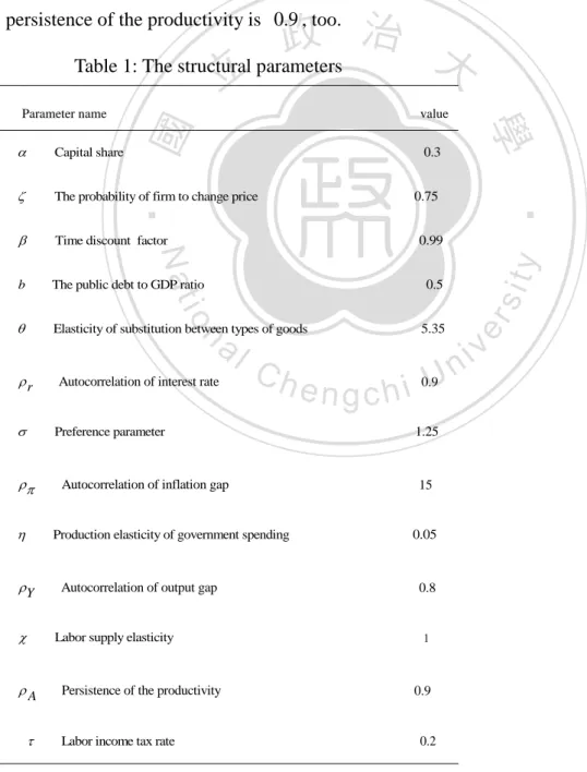
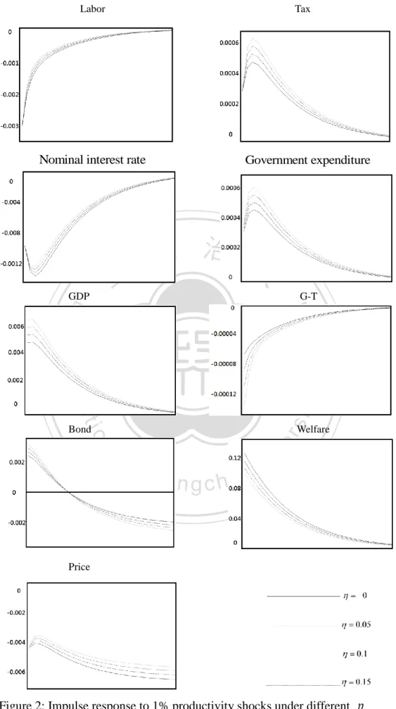
(25) 4. Dynamics. 4.1 Productivity shock Here, we discuss impulse response function when there is an exogenous shock in closed economy. We set the same benchmark parameter as above. The exogenous process follows the first-order autoregressive process, AR(1) , and the persistence of productivity is assumed to be 0.9 . The standard deviations of productivity is 0.01 . Under the benchmark we assumed above, the impulse response functions are listed as below:. 立. 政治大. ‧. ‧ 國. 學. n. er. io. sit. y. Nat. al. Ch. engchi. Figure 1: Impulse response function 13. i n U. v. 13. In figure 1, The horizontal axis means response period, and the vertical axis means the level of impulse reaction. 19.

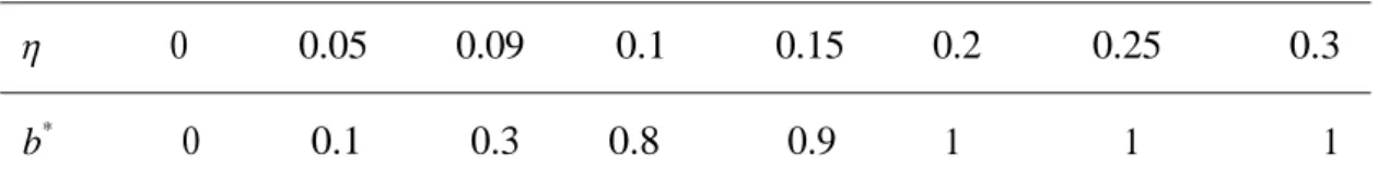
(26) Where rr is the real interest rate in Figure 1, which is positive response if there is a positive productivity shock. There are some variables which have the same response, such as output, consumption, government expenditure, bond, real wage, tax, and welfare. But there are different alterations as labor, marginal cost, long run price, and nominal interest rate. When the economy incurs positive exogenous technology shocks, output will increase. With the wealth effect of output increases, consumption increases, labor supply decreases, and tax base increases. Besides, the government will help output by. 政治大 decreased, and marginal cost decreased also makes consumer price index decreased. 立 raising purchase on capital or increasing public building, which makes marginal cost. ‧ 國. 學. But labor supply decreased makes wage rise. Here government expansionary fiscal expenditure which also need government to borrow by adding bond sell, so that the. 4.2 Sensitivity analysis. al. er. io. sit. y. Nat. buy public bond.. ‧. Fed will decrease the nominal interest rate to induce the representative household to. n. v i n Here, we compare the impulse of variables under different Cresponse h e n gfunction i h c U.  as. Figure 2. First, we observe a phenomenon on the positive variable level of real output and consumption, the effect of  increases will make them decline more.14 With government productivity increase, the negative variable of labor supply will increase, and the positive variable of T and government expenditure will decline. Since the level of G  T impulse response increases with an increase in  . That is, the more government expenditure needs more tax with an increase in  , but the labor supply decreases which makes the tax based less, so that the government faces the fiscal. 14. We had discussed above, which denote that Leeper, Walker, and Yang (2009) also have the same result. 20.

(27) dilemma. Hence, the government will issue public debt to finance the deficit, and we can find the bond will become more with  increases. Moreover, Government needs more revenue if  increases, hence central bank has to reduce the nominal interest rate more to induce individuals to buy public bond for government expenditure, and the negative variable level of nominal interest rate impulse response is more with an increase in  . The positive variable level of real GDP is smaller with  increases, but the negative variable level of price is greater. Since b = Bt / ( PY t t ) , the positive variable. 政治大. level of nominal bond quantity is smaller, The positive variable level of welfare is. 立. greater with an increase in  .. ‧. ‧ 國. 學. n. er. io. sit. y. Nat. al. Ch. engchi. 21. i n U. v.

(28) Labor. Tax. Nominal interest rate. 立. GDP. Government expenditure. 政治大 G-T. ‧. ‧ 國. 學 sit. y. Nat. Welfare. n. al. er. io. Bond. Ch. engchi. i n U. v. Price. Figure 2: Impulse response to 1% productivity shocks under different  22.

(29) 5. Welfare Measure. 5.1 The Welfare Criterion Here, we measure the level of utility under different policy regimes. Now we follow Schmitt-Grohe and Uribe (2007), and construct a conditional expectation utility function as the welfare measure.15.  Ct1 L1t  W0  E0     . t 0  1   1   . t. 政治大 steady-state values of labor supply and consumption to get W 立. That is, we calculate the expected lifetime utility on the initial state. So we use the 0. as the welfare state at. ‧ 國. 學. time zero. Then we follow Lucas (1987) and assume that Wa is the welfare under policy regime a as:. y. Nat.   , . io. sit. t. ‧.  Ct1,a L1t,a Wa  E0     t 0  1   1  . er. where Ct ,a and Lt ,a mean consumption and labor supply under policy regime a .. al. n. v i n Now we denoted the decreasedCproportion of consumption as hengchi U.  , and  means the. variation between policy regime a and the initial state. Therefore, we can describe. the difference as:   ((1   )C ss )1 ( Lss )1 Wa  E0   t   1 1  t 0 .  . . If the proportion  is higher, then the welfare is lower.. 15. Teo (2010), also use the same way to calculate the welfare at initial time and evaluate the welfare criterion under a given policy regime a . 23.

(30) Table 5: The welfare loss  among the different b. b. 0. 0.1. 0.2. 0.3.  -0.050287 -0.050303 -0.050254. -0.050057. 0.4. 0.5. -0.050078. -0.050056. 0.6 -0.049907. 0.7. 0.8. 0.9. 1. -0.049908. -0.049799. -0.049768. -0.049643. 5.2 Welfare Analysis of Optimal Policy Here, we solve  on the benchmark but deferent debt ratio from zero to one as Table 5. Interestingly, when b is 0.1 ,  is the smallest. Therefore, the optimal debt ratio is 0.1 under our benchmark. That is, the government wants to hold the debt-GDP. 政治大. ratio to be 10% in the long run.. 立. 5.3 The Optimal Policy under different government productivity. ‧ 國. 學. Then we try to find the optimal debt ratio under different elasticity of government. ‧. expenditure. As shown in Table 6, 16 the optimal debt ratio increases with . sit. y. Nat. increases, and the optimal debt ratio increases quickly as   0.1 . The reason is . al. er. io. increases which mean the government expenditure will heighten to help product.. v. n. Besides, a change in  which also influences the firm to change the employment of. Ch. engchi. i n U. people since the set of production function. Since the government expenditure is heightened too high to be covered by the tax revenue, so that government will raise the debt ratio to offset the government purchase. When   0.05 , government productivity is very small so that the government does not need to hold more debt to balance the budget constraint. Table 6: Optimal debt ratio under different .  b* 16. 0. 0 We put all. 0.05. 0.09. 0.1. 0.15. 0.2. 0.25. 0.1. 0.3. 0.8. 0.9. 1. 1.  under different debt-ratio and  in the Appendix. 24. 0.3 1.

(31) Hence, optimal debt ratio is zero when  equals zero, we can find the same result in previous studies. So the optimal debt ratio rises with  increases, and the optimal debt ratio increases quickly after   0.1 . The reason that we can find in equation as below, MPG . Y Y .  G G. Where we rewrite the equation to. G MPG   , where MPG is marginal production Y. of government expenditure. That is, when the government expenditure to GDP ratio is fixed, the  will influence the MPG . Hence an increase in  makes the MPG. 政治大 increased, but the government expenditure also needs more revenue to balance the 立. fiscal policy. Hence, the government has to raise the ceiling of debt ratio to reach. ‧ 國. 學. balanced budget fiscal. The reason is that the government helps firm to produce or. ‧. constructs building which requested a huge expenditure. Besides, there is the wealth. sit. y. Nat. effect if  increases, which made the labor supply to decrease. Labor supply. io. al. n. issuing public bond.. er. decreases which also led tax base to reduce, hence government should borrow by. Ch. engchi. 25. i n U. v.

(32) 6. Conclusion The purpose of this paper is to find an optimal debt ratio in a closed economy under the DSGE framework. We follow Barro (1988) to introduce government department into firm’s production. The authority can enhance firm’s productivity by increasing the infrastructure (capital goods, constructing public building, increasing education spending, and legislating law). We find that optimal debt ratio will increase when the production elasticity of government expenditure increases. That is, the government budget should be balanced by debt financing when government productivity is raised.. 政治大 decreases and hence government expenditure could not be sustained by declining tax 立. The wealth effect of government productivity growth also causes labor supply. revenue. So that government issues public bond to finance. And the quantity of public. ‧ 國. 學. bond will increase if the production elasticity of government expenditure increases.. ‧. In 2012, the U.S. faces a terrible finance crisis, and Krugman and among others. sit. y. Nat. argued that the government should raise expenditure and increase debt, but eventually. io. er. the Obama government reduced the fiscal expenditure and lifted the debt ceiling. According to this paper, we suggest that the U.S. government should increase more. al. n. v i n C hincrease debt ratio.U But we still have a question expenditure on infrastructure and engchi which we should solve, that is, the optimal production elasticity of government expenditure value. This is for future work.. 26.

(33) Reference. Aiyagari, S. R. and McGrattan, E.R., 1997. The optimum quantity of debt. Federal Reserve Bank of Minneapolis Research Department Staff Report 203. Arrow, K.J. and Kurz, M., 1970, Public Investment, the Rate of Return and Optimal Fiscal Policy, Baltimore, MD: Johns Hopkins University Press. Aschauer, D.A., 1988. Is public expenditure productive? Journal of Monetary Economics Vol. 23, 177-200. Barro, R.J., 1974, Are government bonds net wealth? Journal of Political Economy, Vol. 82, No. 6, 1095-1117.. 立. 政治大. ‧ 國. 學. Barro, R.J., 1979. On the determination of the public debt. Journal of Political Economy, Vol. 87, No. 5, part 1, 940-971.. ‧. Barro, R.J., 1988. Government spending in a simple model of endogenous growth. National Bureau of Economic Research 1050, Massachusetts Avenue.. y. Nat. sit. n. al. er. io. Barro, R.J. and Sala-I-Martin, X., 1992. Public finance in models of economic growth. Review of Economic Studies, Vol. 59, Issue 4, 645-661.. Ch. i n U. v. Baxter, M. and King, R.G., 1993. Fiscal policy in general equilibrium. American Economic Review, Vol. 83, No. 3, 315-334.. engchi. Button, K., 1998. Infrastructure investment, endogenous growth and economic convergence. The Annals of Regional Science, Vol. 32, 145-162. Devereux, M., 2010. Fiscal deficits, debt, and monetary policy in a liquidity trap. Central Bank of Chile Working Papers, No. 581. Evans, P. and Karras, G., 1994. Are government activities productive? Evidence from a panel of U.S. states. Review of Economics and Statistics, Vol. 76, No1, 1-11. Finn, M., 1993. Is all government capital productive? Federal Reserve Bank of Richmond Economic Quarterly, Vol. 79/4, 53-80. 27.

(34) Fisher, W. and Turnovsky, S., 1998. Public investment, congestion and private capital accumulation. Economic Journal, Vol. 108, 339–413. Gramlich, E.M., 1994. Infrastructure investment: A review essay. Journal of Economic Literature, Vol. 32, No. 3,1176-1196. Greiner, A., 2010. Economic growth, public debt and welfare: comparing three budgetary rules. German Economic Review, Vol. 12, No. 2, 205-222. Holtz-Eakin, D., 1994. Public-sector capital and the productivity puzzle. Review of Economic and Statistics, Vol.76, No. 1, 12–21. Juillard, M., Karam, P., Laxton D., and Pesenti, P., 2006. Welfare-based monetary policy rules in an estimated DSGE model of the US economy. International Research Forum on Monetary Policy Working Paper Series, No. 613.. 立. 政治大. ‧ 國. 學. Kamps, C., 2004. The Dynamic Macroeconomic Effects of Public Capital. Springer, Berlin, Germany.. ‧. sit. y. Nat. Lansing, K.J., 1998. Optimal fiscal policy in a business cycle model with public capital. The Canadian Journal of Economics, Vol. 31, No. 2, 337-364.. n. al. er. io. Leeper E.M., Walker T.B., and Yang S.C. S., 2009. Government investment and fiscal stimulus. Journal of Monetary Economics, Vol. 57, 1000-1012.. Ch. engchi. i n U. v. Linnemann L. and Schabert A., 2006. Productive government expenditure in monetary business cycle models. Scottish Journal of Political Economy, Vol. 53, No. 1, 28-46. Lucas, R., 1987. Models of Business Cycles. Yrjö Johansson Lectures Series. London: Blackwell. Malley, J., Philippopoulos, and A., Woitek, U., 2009. To react or not? Technology shocks, fiscal policy and welfare in the EU-3. European Economic Review, Vol. 53, 689–714. Martin, F. M., 2009. A positive theory of government debt. Review of Economic Dynamics, Vol. 12, 608-631. 28.

(35) Mayer, E., Moyen, S., and Stahler. N., 2010. Government expenditure and unemployment a DSGE perspective. Deutsche Bundesbank, Wilhelm-Epstein-StraBe 14, 60431 Frankfurt am Main. Minea, A. and Villieu, P., 2009. Borrowing to finance public investment? The ‘Golden Rule of Public Finance’ reconsidered in an endogenous growth setting. Fiscal Studies, Vol. 30, No. 1, 103-133. Nadiri, M.I. and Mamuneas, T.P., 1994. The effects of public infrastructure and r & d capital on the cost structure and performance of us manufacturing industries. Review of Economic and Statistics, Vol. 76 , No.1, 22–37. Ratner, J.B., 1983. Government capital, employment and the production function for US private output. Economic Letters, Vol 13, 213–217. 立. 政治大. ‧ 國. 學. Schmitt-Grohe, S. and Uribe, M., 2007. Optimal simple and implementable monetary and fiscal rules. Federal Reserve Bank of Atlanta Working Paper Series 2007-24.. ‧. Sturm, JE, de Haan J, 1995. Is public expenditure really productive? New evidence for the USA and the Netherlands. Economic Modelling 12, 60–72.. y. Nat. sit. n. al. er. io. Taylor, J.B., 1998. The robustness and efficiency of monetary policy rules as guidelines for interest rate setting by the European central bank. Conference on Monetary Polocy Rules, Stockholm, June 12-13, 1998.. Ch. engchi. i n U. v. Teo, W.L., 2010. Inventories and optimal monetary policy in a small open economy.. Traum, N. and Yang, S.C. S., 2010. When does government debt crowd out investment? Center For Applied Economics And Policy Research Working paper, 006.. 29.

(36) Appendix. A.  under different debt-ratio and . . b 0. 0.1. 0.2. 0.3. 0.4. 0.5. 0.7. 0.8. -0.047749. -0.047556. 0.9. -0.048404. -0.048299. -0.048181. -0.047956. -0.047994. 0.05. -0.050287. -0.050303. -0.050254. -0.050057. -0.050078. -0.050056. -0.049907. -0.049908. -0.049799. -0.049768. -0.049643. 0.09. -0.051911. -0.051889. -0.051904. -0.051971. -0.051928. -0.051878. -0.051835. -0.051815. -0.051832. -0.051816. -0.051871. 0.10. -0.052351. -0.052410. -0.052433. -0.052349. -0.052345. -0.052266. -0.052387. -0.052293. -0.052434. -0.052309 -0.052283. 0.15. -0.054675. -0.054774. -0.054875. -0.054920. -0.054934. -0.055027. -0.054976. -0.055144. -0.055140. -0.055329 -0.055323. 0.20. -0.057058. -0.057296. -0.057289. -0.057638. -0.057654. -0.05786. -0.058215. -0.058115. -0.058487. -0.058570. 0.25. -0.059855. -0.060016. -0.060321. -0.060666. -0.061025. -0.061295. -0.061377. -0.061712. -0.061972. -0.062369 -0.062579. 0.30. -0.063133. -0.063256. -0.063486. -0.064107. -0.064600. -0.064741. -0.065262. -0.065721. -0.066267. -0.066467 -0.066986. 政治大. -0.047440 -0.047399. 1. 0.00. 立. -0.047925. 0.6. ‧. ‧ 國. 學. n. er. io. sit. y. Nat. al. Ch. engchi. 30. i n U. v. -0.047157. -0.05865.

(37)