鐵─鎳─鎵合金材料的鐵磁共振與磁彈性質研究

國立交通大學

電子物理研究所

博士論文

鐵─鎳─鎵合金材料的鐵磁共振與磁彈性質研究

Ferromagnetic resonance and magneto-elastic

properties of (FeNi)

81

Ga

19

alloys

研 究 生:劉奇青

指導教授:任盛源 教授

莊振益 教授

鐵─鎳─鎵合金材料的鐵磁共振與磁彈性質研究

Ferromagnetic resonance and magneto-elastic properties of

(FeNi)

81

Ga

19

alloys

研 究 生:劉奇青 Student : Chi-Ching Liu 指導教授:任盛源 教授 Advisor: Shien-Uang Jen 莊振益 教授 Advisor: Jenh-Yih Juang

國立交通大學

電子物理研究所

博士論文

A Dissertation

Submitted to Department of Electrophysics College of Science

National Chiao-Tung University in Partial Fulfillment of Requirements for the Degree of Doctor of Philosophy

in Electrophysics

October 2013 Hsinchu, Taiwan

I 鐵─鎳─鎵合金材料的鐵磁共振與磁彈性質研究 研 究 生:劉奇青 指導教授:任盛源 教授 莊振益 教授 國立交通大學 電子物理研究所

中文摘要：

本實驗計畫為，鐵─鎳─鎵合金材料鐵磁共振與磁彈性質的研究。其中， 在膜材的研究方面，我們是利用磁控濺鍍在基板上沉積成薄膜，我們分別 沉積系列合金Fe81-xNixGa19於矽基板上，和沉積系列合金Fe81-yNiyGa19於玻

璃基板上，其中x、y為 0 到 26。我們已經做的量測主要為：(1)磁滯伸縮的 量測、(2)易軸、難軸的磁滯曲線、(3)鐵磁共振的實驗。鐵磁共振在 9.6GHz 的交變磁場下執行，透過Kittle模型我們可以得到自然共振頻率，再透過磁 滯曲線的資訊我們可以得到Gilbert阻尼係數。在薄膜的實驗中，我們得到幾 個材料的特性：(1)在系列合金中，磁異向場隨鎳的原子百分比增加而降低、 (2)自然共振頻率隨鎳的增加而降低、(3) Gilbert阻尼係數亦隨鎳的原子百 分比增加而降低、(4)磁致伸縮的峰值出現在鎳原子百分比為 22 的時候。 其中，特性(1)、(2)和(3)皆因為鎳元素取代鐵元素時降低其合金的磁性， 因而降低了磁異向能量，磁異向場亦隨之降低，進而牽動自然共振頻率與 Gilbert阻尼係數。特性(4)系因鎳的添加而改變了薄膜的晶相，進而提升薄

II 膜的磁致伸縮。至此，我們發現Fe59Ni22Ga19 Yager、Galt和Merritt指出鐵磁共振的半高寬與磁異向場大小有關，其實 驗證明磁異向場越大，則鐵磁共振半高寬越寬，而在系列和金中增加鎳原 子百分比可有效降低磁異向場，進而得以降低Gilbert阻尼係數。另外，由 XRD的數據顯示，系列合金中鎳原子百分比的增加可有效抑制D0 在玻璃上有很優良的磁彈性質 並可以在微波中應用。 19 相與 L12 相的生成，證據顯示，甚至在鎳原子百分比達到 22 百分比時，合金薄 膜中僅存在A2 相，D019 相與 L12 另外，此篇論文也針對Fe 相其磁伸縮值皆為負值，不利合金薄膜 飽和磁伸縮最佳化，從實驗數據中我們也得到鎳原子百分比達到 22 百分比 的系列合金，有最佳化的飽和磁致伸縮值。 81-zNizGa19系列合金薄帶做一系列的探討，其 中z為 0 到 24。薄帶樣品是由快速冷淬法所製備而成，由XRD數據顯示，材 料的晶格常數與鎳成分的添加有對應關係。由磁滯曲線的觀察，當合金薄 帶添加鎳以後，磁異向性能量降至零，變成等向性質的磁性材料，卻也分 別降低與提高飽和磁化量和矯頑磁力。從磁彈性質的研究中，我們發現楊 氏係數隨鎳原子百分比的增加而降低，並由∆E效應，使觀察到於系列合金 中添加元素鎳的所產優勢，這優勢更進而影響磁致伸縮的大小，我們發現 在鎳佔原子百分比為 7 時，擁有最大的磁致伸縮量。於此結果我們認為 Fe74Ni7Ga19合金薄帶有很優良的磁彈性質並可製成元件加以應用。

III

於鐵─鎵合金中添加鎳元素可以有下降低其的磁異向性，在薄帶研究中， 甚至發現鎳元素的添入更可使材料變成等向性，而正是對軟磁材料的應用 層面相當有利的一個條件。

IV

Ferromagnetic resonance and magneto-elastic properties of (FeNi)81Ga19

alloys

Student : Chi-Ching Liu Advisor: Prof. Shien-Uang Jen Prof. Jenh-Yih Juang

Department of Electrophysics National Chiao-Tung University

Abstract:

Fe81-xNixGa19/Si(100) and Fe81-yNiyGa19/glass films, where

x or y = 0 - 26, were made by the magnetron sputtering method. We have performed three kinds of experiments on these films:

[i] the saturation magnetostriction (λS) measurement; [ii] the easy-axis and

hard-axis magnetic hysteresis loop measurements; [iii] the ferromagnetic resonance (FMR) experiment to find the resonance field (HR) with an X-band

cavity tuned at fR = 9.6 GHz. The natural resonance frequency, fFMR

The main findings of this study are summarized:

, of the Kittel mode at zero external field (H = 0) was then obtained and used to calculate the Gilbert damping constant.

[i] HK decreases, as x or y increases; [ii] fFMR decreases, as x or y increases;

[iii] α decreases from 0.052 to 0.020 and then increases from 0.020 to 0.050, as x increases, and α decreases from 0.060 to 0.013, as y increases; [iv] λS reaches

maximum when x = 22. The reason of the [i], [ii] and [iii] are described below: as addition Ni replaces Fe at.% in alloys magnetism in rich-Fe alloys is reduced. As a result, the magnetic anisotropy energy causes the HK to decrease,

and, therefore, fFMR and α also decrease. The reason of [iv]: as addition Ni into

V

Thus, we conclude that the Fe59Ni22Ga19

Yager, Galt, and Merritt pointed out that ΔH is related to H

/glass film should be suitable for the magneto-electric microwave device applications.

K. Besides, we

find the addition of Ni into Fe81Ga19 alloy films destabilize the D019 phase and

L12 phase. Briefly speaking, when y = 22 at.%Ni, there is only one single A2

phase. That centralized the HR and narrow ΔH in the alloys. In Eq. (2), α of

the FeNiGa alloy is calculated from ΔH; α decreases, as ΔH decreases. On the other hand, the Fe81Ga19 film with the D019 phase and L12 phase are detrimental

to saturation magnetostriction, so we get magnetostriction constants in the FeNiGa ternary alloys higher than those of the Fe81Ga19

Another series of Fe

binary alloys.

81-zNizGa19 ribbons, where z = 0 - 24, were made by the

rapidly quenching method. The X-ray diffraction patterns showed that these ribbons change the lattices constants which depend on number of z. From hysteresis loops information, the ribbons become isotropic in magnetic anisotropy, Ms decreases from 170 emu/g to 116 emu/g, and Hc inceases from

4.8 Oe to 11.7 Oe, as Ni is added in. Young’s modulus (Es) at magnetization

saturation and ∆E effect were estimated from the strain curve. We discovered that as z increases, ∆E/E0 increases. The most important result is that

λ reaches maximum when z = 7 at.%Ni. We conclude that the Fe74Ni7Ga19

The addition of Ni into Fe

ribbon should be most suitable for the magneto-electric device application.

81Ga19 alloys refined the magnetic anisotropy

energy which let the HK decreases, as Ni content increases. Even in the series

VI

誌謝

首先要感謝，中央研究院物理所 任盛源老師對學生的費心，無論是研 究上或是生活上，老師總是傳承經驗，並且不吝惜的給予指導；更一步步 在實驗中訓練學生對實驗的敏銳度及嚴謹的態度，這將會是學生一輩子受 用不盡的寶藏。此外也要特別感謝，交通大學電子物理系 莊振益老師對 學生的指導，總是能見微知著的給予學生建議，適時的引導方向，更讓學 生明瞭細節的重要性，相信這將會是將來能夠推動學生能百尺竿頭更進一 步的動力。 再來要感謝交大的原銘、家宏、培元、韋呈、皓葦學長及中研院的宗霖 學長，總是能在課業上給予幫助，並在研究中提出一些獨到的見解，使本 人有更多元的視野。也要感謝交大的同儕雁夫、君緯，記得修課時，一起 寫作業、一起熬夜念書、一起找出答案的日子，後來也常常在本人的研究 中提出意見，更能激發很多思考的新方向。除了學業上的幫助，也要謝謝 學長、同學及學弟妹在課餘時間所提供的歡樂，總是能讓本人在疲憊之後 能重新打起精神繼續前進。 最後要感謝我的家人，尤其是父親劉元森先生與母親李碧釵女士，在不 算短的學生生涯裡，提供不虞匱乏的生活，從不用為了日子而煩惱，這份 養育的恩情是求學過程中最大的助力。並感謝我的妹妹玠玫，在成長的過

VII

程中與我的互相省思，使我能更確定自己要走的路，更要感謝從不曾怨懟 我仍未負擔家計，不給我這方面的壓力，使我能沒有顧慮的完成學業。當 然，還要感謝一路上相互扶持，幫我加油打氣的朋友，有你們真好。

VIII

Contents

Abstract (in Chinese)………...…....I Abstract (in English)………...…IV Acknowledgement………....…...…VI Contents………..……….VIII Figure and Table Lists………...……...XI

Chapter 1 Introduction……….….…….1

1.1 Magneto-Electric Microwave Device………...1

1.2 Fundamental Properties of Fe-Ga alloys………....…..….4

1.3 Motivation………...……..6

Chapter 2 Brief review of magnetism and relevant effects………9

2.1 Magnetism………9

2.2 Ferromagnet……….…15

2.2.1 Soft magnetic materials and Hard magnetic materials…...…19

2.2.2 Curie temperature………..…20 2.3 Magnetic anisotropy………..…………...……21 2.3.1 Crystal anisotropy………...…21 2.3.2 Shape anisotropy………...…23 2.3.3 Stress anisotropy………...………24 2.3.4 Induced anisotropy………..………….……….24 2.4 Magnetostriction………...……….26

IX

2.4.1 Measure λ on bulk or ribbon………...…29

2.4.2 Measure λ on thin film………....31

2.5 Ferromagnetic Resonance………...…….32

2.6 Skin effect………...….35

Chapter 3 Experimen

ts

………...………...36

3.1 Process………...36

3.1.1 Samples for film………...……….36

3.1.2 Samples for ribbon………....37

3.2 DC magnetron sputtering method………...…...38

3.2.1 Process conditions………...…...39

3.3 Rapid quenching melt-spun method………..……41

3.4 The Dektak3 3.5 X-ray diffraction (XRD)………...…….46

system………..…….….43

3.6 Nano-indentation system measure………...…..48

3.7 Electrical resistivity measurement……….50

3.8 Ferromagnetic resonance (FMR) experiments………...……52

3.9 Vibrating-Sample Magnetometer (VSM)………...…………54

3.9.1 Measuring hysteresis loops………...…56

3.10 Magnetostrictions………..………..…………..59

3.10.1 Optical-cantilever magnetostriction experiment for films……….59

3.10.2 Magnetostriction experiment for a ferromagnetic ribbon sample……….…61

Chapter 4 Results and discussion for films………..64

X 4.2 FMR data………65 4.3 Magnetostrictions data……….…………77 4.3.1 Young’s modulus (Ef 4.3.2 Main data………..……….78 ) data………...……….77

Chapter 5 Results and discussion for ribbons……….80

5.1 XRD data………..………..80

5.2 VSM results………..……..83

5.3 Electrical resistivity………..………..87

5.4 Young’s modulus of the ribbon………...………...88

5.5 Magnetostrictions data………...…………92 Chapter 6 Conclusions………..96 6.1 For Films………...……….96 6.2 For Ribbons………..……….98 Chapter 7 Appendix……….99 7.1 XRD discussion………..99

7.2 TEM photo for the Fe70Ni11Ga19/Si(100) film……….………..102

7.3 σ vs. ∆ε of the Fe68Ni13Ga19 ribbon………..……….104

Reference………...…105

XI

Figure and Table Lists

Fig. 1.1 shows the schematic illustration of the Barkhausen effect………...3 Fig. 1.2 Conventional types of in transformer cores………...3 Fig. 1.3 Room temperature magnetostriction of Fe1−xGax alloys quenched into

water from 800o

Fig. 1.4 The XRD patterns for FeGaB films with different B contents ……...5 C………....5

Fig.1.5 The cross-section TEM photos for Fe85Ga15 and Fe78Ni7Ga15

Fig. 1.6 Magnetostriction measured on stacked Fe

ribbons………..……..7

85Ga15

Fig. 1.7 Magnetostriction measured on stacked ribbons of Fe

ribbon, applying the field parallel to the ribbon thickness………...……7

78Ni7Ga15

Fig. 2.1 Bar magnet in a uniform field………...……….14 applying the field parallel to the ribbon thickness………..………8

Fig. 2.2 Domain structure of a polycrystalline specimen model…………....17 Fig. 2.3 The Bitter method image, which was taken in a zero field and at room

temperature, of the Fe81Ni19

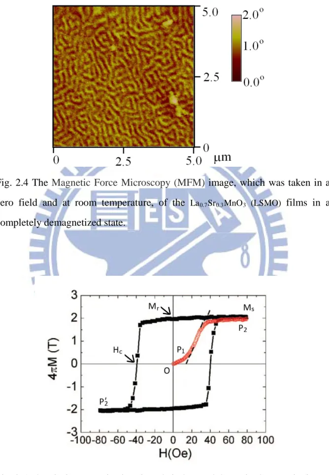
Fig. 2.4 The Magnetic Force Microscopy (MFM) image, which was taken in a zero field and at room temperature, of the La

array films in a completely demagnetized state………..…………..17

0.7Sr0.3MnO3

Fig. 2.5 The virgin magnetization (in red circles) and the major hysteresis (in black squares) curves of the Fe

(LSMO) f i l m s i n a c o m p l e t e l y d e m a g n e t i z e d s t a t e … … … 1 8

86V14 film. 4πM is the magnetization

XII

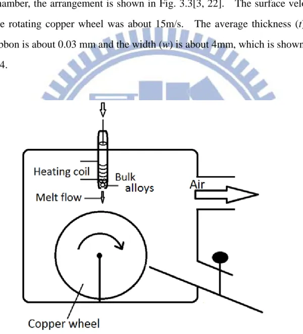
Fig. 2.6 This figure is the soft ferromagnetic material hysteresis (in red circles) and the hard ferromagnetic material hysteresis (in blue squares)

curves………..…...20

Fig. 2.7 Magnetization curves of single-crystal of iron………...……22

Fig. 2.8 Magnetization curves of single-crystal of nickel…………...……22

Fig. 2.9 Magnetization curves of single-crystal of cobalt…………..………23

Fig. 2.10 shows dependence of magnetostriction on magnetic field…..……28

Fig. 2.11 indicates magnetostriction of an iron crystal in the [100] direction……….…...29

Fig. 2.12 Magnetostriction measurement on a sample (bulk or ribbon) using a strain gage………..30

Fig. 3.1 Thin film prepared by dc magnetron sputtering………...39

Fig. 3.2 shows schematics of the Sputtering system………...……40

Fig. 3.3 Ribbons preparation by rapid quenching melt-spun…………...41

Fig. 3.4 The samples of ribbon are made by the rapid quenching melt-spun method……….…………..42

Fig. 3.5 shows Dektak3 Fig. 3.6 Block diagram of Dektak system………44

3 Fig. 3.7 The schematic illustration of Bragg's law………..46

architecture………..45

Fig. 3.8 The X-ray diffraction figure on series of Fe81-yNiyGa19 Fig. 3.9 The X-ray diffraction figure on series of Fe /glass films………...……47

8 1 - zNizGa1 9 Fig. 3.10 Nano-indentation system………..49

XIII

Fig. 3.11 Solid curves represent the best-fit results of E vs. hP, where E is the

Young′s modulus and hp

Fig. 3.12 Measure the

is the depth of circle of contact, obtained from the nano-indentation measurements, for the Fe-Ni-Ga/glass films……….…..49 resistivity by the collinear four-probe array...…50 Fig. 3.13 Ferromagnetic resonance model………...52 Fig. 3.14 A typical FMR absorption spectrum of the Fe70Ni11Ga19

Fig. 3.15 Vibrating sample magnetometer (VSM) model………...………55 /Glass film at the microwave frequency f = 9.6 GHz………....53

Fig. 3.16 Vibrating-Sample Magnetometer (VSM).

Courtesy Lake Shore Cryotronics, Inc………...……….56 Fig. 3.17 The in-plane rotation SQR data of the Fe81Ga19

Fig. 3.18 (a) The hard-axis (HA) and (b) the easy-axis (EA) magnetic hysteresis loop of the Fe

/Si film…..…....57

55Ni26Ga19film deposited on a glass substrate. HK is the

anisotropy field, 4πMS is the saturation magnetization, HC is the coercivity,

and (SQR)HA and (SQR)EA

Fig. 3.19 Optical-cantilever magnetostriction experiment system……...60 are the squareness ratio along HA and EA, respectively………....58

Fig. 3.20 The x-direction and y- direction Helmholtz coils…………..…….60 Fig. 3.21 Typical hysteresis loops for longitudinal and transverse

magnetostrictions (λ∥ and λ⊥) of the Fe59Ni22Ga19/glass film plotted as a function of the external field H………...61 Fig. 3.22 A photo of the experimental set-up for the stress-strain (σ-∆ε) and

magnetostriction (λ) measurements………..…..63 Fig. 4.1 The main resonance field (HR

Fig. 4.2(a) Magnetic anisotropy field (H

), at f = 9.6 GHz, the various FeNiGa films……….…..72

K) decreases, as at% Ni increases of the

XIV

Fig. 4.2(b) Natural resonance frequency (fFMR

Fig. 4.3(a) Static rotational permeability (µ

) of the FeNiGa films plotted vs. the Ni concentration (x or y)……….73

R

Fig. 4.3(b) The products, µ

) increases, x or y increases in the FeNiGa films……….………73

R×(fFMR) 2

Fig 4.4 shows dependence of the real and imaginary part of the rotational susceptibility on the intensity of the dc field about the resonance field. The maximum χ" occurred at φ = 90

≒constant, x or y increases in the FeNiGa films………...74

o

, and the width of the absorption curve at half the maximum value or a half-value width correspond at φ = 45o

Fig. 4.5 Gilbert damping parameter (α) plotted as a function of the Ni concentration (x or y) for the FeNiGa films……….…..…...75

………..….74

Fig. 4.6 Electrical resistivity (ρ) is about 120 - 150 µΩcm for FeNiGa films deposited on insulating glass………...76 Fig. 4.7 This is Young′s modulus of the two series of Fe81-xNixGa19/Si(100) and

Fe81-yNiyGa19

Fig. 4.8 Saturation magnetostriction (λ

/glass films, respectively……….………77

S

Fig. 4.9 The t

) reaches maximum, when x or y = 22 at.%Ni………79

f dependence of λS of the Fe59Ni22Ga19/Si(100) and

Fe59Ni22Ga19

Fig. 5.1 The lattices constant of melt-spun Fe

/glass films………...………….79

81Ga19 be calculated by the red line

c r o s s y - a x i s . T h e l a t t i c e c o n s t a n t o f t h i s r i b b o n i s 2.925 Å………...………...82

XV

Fig. 5.2 The lattice constant first decreases from 2.925 Å to 2.900 Å and then stabilizes around 2.900 Å for the FeNiGa ribbons……….….82 Fig. 5.3 The easy-axis (θ=0o

melt-spun Fe

) hysteresis loops of the

81Ga19

Fig. 5.4 shows Saturation magnetization (M

………..….84

s), coercivity (Hc), and saturation

field (Hs) hysteresis of the melt-spun Fe81-zNizGa19

Fig. 5.5 Electrical resistivity (ρ) of the melt-spun Fe

...86

81-zNizGa19

Fig. 5.6 The stress (σ) vs. strain (∆ε) curves of the as-spun Fe

………….87

81Ga19

Fig. 5.7 The Young’s modulus in the saturated state (E

ribbon……….90

s

Fig. 5.8 The ∆E effects of the melt-spun Fe

) plotted as a function of z……….………90 81-zNizGa19 F i g . 5 . 9 T h e c r i t i c a l i n t e r n a l s t r e s s (σ ………...91 i c ) o f t h e m e l t - s p u n Fe81-zNizGa19

Fig. 5.10 Magnetostriction of the Fe

……….………...91

81Ni3Ga19

Fig. 5.11 Under the 6 kOe external field, plotted the ∆λ VS. w for the series of the melt-spun Fe

ribbon plotted as a function of a h o r i z o n t a l i n - p l a n e f i e l d u n d e r a n e x t e r n a l w e i g h t w = 208.6 g………..…....94

81-zNizGa19

Fig. 5.12 The melt-spun Fe

ribbons……….…....94

81-zNizGa19 saturation magnetostriction (λs) is

calculated by ∆E/E0, Es and σic

Fig. 7.1 XRD pattern of the FeGa alloy film on Si(100) substrate…..….100 ………..…..…..95

Fig. 7.2 XRD pattern of the Fe57Ni24Ga19

Fig. 7.3 MTG scans of the Fe

ribbon with the quenching rate (rotating copper wheel speed) was about 15m/s…………...…...100

XVI

Fig. 7.4 The cross-section transmission electron microscopy photo of the Fe70Ni11Ga19/Si(100) film. (a) The Fe70Ni11Ga19 alloys deposited on Si(100)

substrate similar pillars. (b) This shows the polycrystal substrate. (c) Shows the Fourier transform pattern

Fig. 7.5 The stress (σ) vs. strain (∆ε) curves of the as-spun Fe

………103

68Ni13Ga19

ribbon………..……….104

Table 3.1 Technical specifications………..………...………..44 Table 3.2 Correction factor C for the calculation of the resistivity measured with c o l l i n e a r f o u r - p o i n t p r o b e s p l a c e d o n a s y m m e t r y axis………...51 Table 4.1 Structural properties, the x-ray diffraction peaks, of the

Fe81-yNiyGa19/glass films. I/Imax

Table 4.2 (∆H)

is the peak intensity ratio. a is the lattice constant……….64

A/(∆H)exp

Table 5.1 Structural properties, the x-ray diffraction peaks, of the Fe

is the degree of asymmetry of the FMR c linewidth………...……….75

81-zNizGa19

ribbons. I/Imax is the peak intensity ratio. a0 is the lattice

1

1. Introduction

1.4 Magneto-Electric Microwave Device

The desirable properties for soft magnetic materials are high permeability (µ) and low loss. The hysteresis loss is the most important loss in ferromagnetic substances at low driving frequencies. This phenomenon, known as the Barkhausen effect, was discovered in 1919. This effect is the strongest on the steepest part of the magnetic hysteresis curve and is evident for sudden and discontinuous changes in magnetization. The curve is shown in Fig. 1.1, where the magnification factor applied to one portion of the curve is of the order of 109. However, in the high frequency case the hysteresis loss becomes less important. Due to the domain wall displacement, which is the main origin of the hysteresis, is mostly damped in this range and is replaced by the rotation magnetization. There is one example shown in Fig. 1.2. The total loss per cycle (Pt) increases with frequency, as expected, but not linearly. (The measurements cannot be carried to higher frequencies, because the skin effect prevents the sample from being fully magnetized.) There is also a substantial discrepancy between the measured eddy-current loss and calculated classically. The difference between these two losses is called the anomalous loss, and may be as large as or even larger than the calculated eddy-current loss. It appears only because the classical calculation of eddy-current loss ignores the presence of domain and domain wall motion, and is therefore under-estimated. Hence, it is reasonable to compare the observed loss with the calculated classical loss and

2

find their difference as the anomalous loss. When the domain structure of the material is taken into account, the calculated eddy-current loss may exceed the classical loss, and the difference between the two is larger the larger the domain size. The difficulty is that the details of the domain structure and of the domain wall motion are not known in an actual sample, so that calculations can only be made for assumed and simplified models. Thus, the next important loss for ferromagnetic metals and alloys is the eddy current loss. Since a power loss of this type increases in proportion to the square of the frequency, it plays an important role in the high frequency, usually the radio frequency, range[1-3]. Moreover, if the frequency is increased further into the microwave range, one will encounter the ferromagnetic resonance (FMR) phenomenon. General speaking, the magneto-electric device is used in microwave which need to reduce the eddy current loss first. So that, reduce the Gilbert damping parameter (α) in the magnetic materials which is the motivation in this study.

In this study, we wish to find soft magnetic materials, which may be used in a tunable magneto-electric microwave device[4] or other rf/microwave magnetic devices. In these devices, the basic requirements for the soft ferromagnetic films are that low coercivity (HC), high saturation magnetization

(4πMS), high saturation magnetostriction (λS), high rotational permeability (µr),

high limiting (or natural resonance) frequency (fFMR), and low Gilbert damping

3

Fig. 1.1 shows the schematic illustration of the Barkhausen effect.

4

1.2 Fundamental Properties of Fe-Ga alloys

From many researching literatures especially Ref. [4], we find that the Fe-Ga alloys seem to be good soft magnetic materials which could be used for the device applications mentioned above. For example, the Fe-Ga alloys are low coercivity soft magnetic materials with low saturation or anisotropy field (HS), about 100 Oe for single crystals (SC) and about 50 Oe for poly-crystals

(PC)[5, 6], high saturation magnetization, about 18 kG[5], high saturation magnetostriction shown in Fig. 1.3, about 200 ~ 400 ppm for SC and about 40 ~ 100 ppm for PC sample[7, 8]. Note that although the FeGa single crystal has large λS value, which is favorable in terms of magneto-electric coupling, its

ferromagnetic resonance line-width (∆H), about 450 ~ 600 Oe[9] at X band, is however yet too large for tuning efficiency. In other words, α of a FeGa single-crystal film is too large. In reaching of Ref. [4], Lou and Insignares added of B atoms into the FeGaB alloys leads to refined grain size and/or a more disordered lattice, and the XRD patterns are shown in Fig. 1.4. Moreover, from a device application point of view, it is usually more laborious to grow a single-crystal than a polycrystalline film. Thus, in this study we shall concentrate on the polycrystalline film case only. Besides, it has been found that incorporation of about 12% of the metalloid element, such as boron (B) or carbon (C), into the Fe81Ga19 alloy would improve λS[10 - 12]. Note, however,

there is a discrepancy between λS ≈ 70 ppm for the (FeGa)88B12 film and λS ≈

5

Fig. 1.3 Room temperature magnetostriction of Fe1−xGax alloys quenched into

water from 800◦C[7].

6

1.3 Motivation

In this study, we chose one series of the Fe81-xNixGa19/Si(100) and another

one series of the Fe81-yNiyGa19/glass films, where x or y ranges from 0 to 26%,

and other series of magnetic metallic ribbons, Fe81−zNizGa19 with z = 0, 3, 7, 13,

and 24. The TEM photos are shown in Fig. 1.5 from Ref. [13], Bormio-Nunes and Sato Turtelli added nickel (Ni) element into the FeGa alloys leading to refined grain size and/or a more disordered lattice. Besides, it has been found that incorporation of the nickel (Ni) element, into the Fe85Ga15

Hopefully, we can get the combinations of the following favorable features, such as low H

alloy would improve magnetostriction, as shown in Fig. 1.6 and Fig. 1.7.

C or HS, high 4πMS, high λS, from one of these FeNiGa ribbons

and/or films for magneto-electric device. On the other hand, we want get the high µr, low ∆H or α, from one of these FeNiGa films for magneto-electric

7

Fig.1.5 The cross-section TEM photos for Fe85Ga15 and Fe78Ni7Ga15

8

Fig. 1.6 Magnetostriction measured on stacked Fe85Ga15 ribbon, applying the

field parallel to the ribbon thickness[13].

Fig. 1.7 Magnetostriction measured on stacked ribbons of Fe78Ni7Ga15 applying

9

2. Brief review of magnetism and relevant effects

2.1 Magnetism

The first writings of magnetism appeared with a kind of mineral called magnetite (Fe3O4

The discovery of two regions named magnetic poles, or sometimes just “poles,” which attracted a piece of iron more strongly than the rest of the magnetite, this discovery was made by P. Peregrines about 1269 A.D. Sometime later, Coulomb (1736-1806) found that there were two types of poles, now called positive or north poles, and negative or south poles. There is always with magnets and felt the mysterious forces of attraction and repulsion between two magnetic poles[3, 16]. The mysterious forces of attraction and repulsion between the two magnetic poles can be felt. This force of attraction and repulsion is proportional to the product of the strength of the poles and inversely proportional to square of the distance between them. This is Coulomb’s law, which can be written mathematically as,

), which has been claimed that the Chinese used it in compasses sometime before 2500 B.C., but the precise date still remained unknown[3, 16].

10

where 𝐹⃑ is the force, p1 and p2

When a magnetic pole creates a magnetic field around it, and this field will then produces a force on second pole nearby. Experiment shows that this force is directly proportional to the product of the pole strength and field strength or field strength or field intensity 𝐻��⃑,

the pole strengths, r the distance between the poles, and 𝑟⃑₀ one unit vector directed along r. The constant of proportionality

k that occurs permits a definition of pole strength, and the proportionality

constant k is equal 1 in the cgs-emu unit.

𝐹⃑ = 𝑘𝑝𝐻��⃑. (2.2)

The equation 2.2 then defines 𝐻��⃑, a field of unit strength is one which exerts a force 1 dyne on a unit pole. A field of unit strength has an intensity of one oersted (Oe).

Besides, a magnet with poles of strength p located near each end and separated by distance l. Suppose the magnet is placed at an angle θ to a uniform field H (Fig. 2.1). Then a torque acts on the magnet, tending to turn it parallel to the field. The moment of this torque is

(𝑝𝐻𝑠𝑖𝑛𝜃) �_{2� +}𝑙 (𝑝𝐻𝑠𝑖𝑛𝜃) �_{2� = 𝑝𝐻𝑙𝑠𝑖𝑛𝜃 (2.3)}𝑙

When H=1 Oe and θ =90o

𝑚 = 𝑝𝑙 (2.4) , the moment is given by

11

where m is the magnetic moment of the magnet. It is the moment of torque exerted on the magnet when it is at right angles to a uniform field of 1 Oe[2, 3, 16].

Consider a piece of iron is subjected to a magnetic field, it becomes magnetized, and the level of its magnetism depends on the strength of the field. We therefore need a quantity to describe the degree to which a body is magnetized. The application of an external magnetic field causes both an alignment of the magnetic moments of the spinning electrons and an induced magnetic moment due to a change in the orbital motion of electrons In order to obtain a formula for determining the quantitative change in the magnetic flux density caused by the presence of a magnetic material, we let 𝑚��⃑_𝑘 Rbe the

magnetic moment of an atom. If there are n atoms per unit volume, we define a magnetization vector, 𝑀��⃑, as

𝑀��⃑ = lim_∆𝑣→0∑𝑛∆𝑣𝑘=1_{∆𝑣 (2.5)}𝑚��⃑𝑘

Where ∆ν is the volume and n is the number of ∆ν[2, 16].

The magnetic properties of a material are characterized not only by the magnitude and sign of 𝑀��⃑ but also by the way in which 𝑀��⃑ varies with 𝐻��⃑. The scalar ratio of these two quantities is called the susceptibility χ :

12

Now they can be roughly classified into three main groups in accordance with their χ values[3, 16, 17].

(1) Diamagnetic, if χ is a very small negative number.

Electrons which constitute a close shell in an atom usually have their spin and orbital moments oriented so that the atom as a whole has no net moment. Thus the monoatomic rare gases He, Ne, Ar, etc., which have closed-shell electronic structures, are all diamagnetic. The macroscopic effect of this is equivalent to that of a negative magnetization that can be described by a negative magnetic susceptibility. The effect is usually very small, and χ for most known diamagnetic materials is in the order of -10-5

(2) Paramagnetic, if χ is a very small positive number.

Arises mainly from the magnetic dipole moments of the spinning electrons. The alignment forces, acting upon molecular dipoles by the applied field, are counteracted by the deranging effects of thermal agitation. Unlike diamagnetism, which is essentially independent of temperature, the paramagnetic effect is temperature dependent, being stronger at lower temperatures where there is less thermal collision. (i.e., Na, Al)

. (i.e., Cu, Hg, Ag)

(3) Ferromagnetic, if χ is a large positive number.

The magnetization of ferromagnetic materials can be many orders of magnitude larger than that of paramagnetic substances. Ferromagnetism can be explained in terms of magnetized domains. I will show more detail in the next section.

13

Besides, engineers are usually concerned only with ferromagnetic materials and need to know the total flux density 𝐵�⃑ produced by a given field, then engineers become the definition in mks system. In addition, engineers are usually only concerned with ferromagnetic materials and the total flux density 𝐵�⃑ produced by a given field. The mks system is generally used as the unit system in engineering application. They often find the 𝐵�⃑, 𝐻��⃑ curve, also called a magnetization curve, more useful than the 𝑀��⃑, 𝐻��⃑ curve. The ratio of B to H is called the permeability µ:

𝜇 = _{𝐻 (}𝐵 _{𝑚 , 𝑖𝑛 𝑚𝑘𝑠 𝑠𝑦𝑠𝑡𝑒𝑚)} 𝐻 (2.7)

When the magnetic properties of the medium are linear and isotropic, the magnetization is directly proportional to the magnetic field intensity:

𝐵�⃑ = 𝜇𝐻��⃑

= 𝜇0(1 + 𝜒)𝐻��⃑

= 𝜇0𝐻��⃑ + 𝑀��⃑ (2.8)

Where µ0

𝜇0 = 4𝜋 × 10−7 �_m�. H (2.9)

is the permeability of free space is chosen to be

14

equation (2.1)

Fig. 2.1 Bar magnet in a uniform field[3].

15

2.2 Ferromagnet

According to the models of magnetized domains, which have been experimentally confirmed, a ferromagnetic material (such as Co, Ni, and Fe) is composed of many small domains, their linear dimensions ranging from a few microns to about 1 mm. These domains, each contain about 1015 or 1016 atoms, are fully magnetized in the sense that they contain aligned magnetic dipoles resulting from spinning electrons even in the absence of an applied magnetic field. Quantum theory asserts that strong coupling forces exist between the magnetic dipole moments of the atoms in a domain, holding the dipole moments in parallel. Between adjacent domains there is a transition region about 100 atoms thick called a domain wall. In a demagnetized state the magnetic moments of the adjacent domains in a ferromagnetic material have different directions, as exemplified in Fig. 2.2 by the polycrystalline specimen model shown[2, 3, 16, 17]. There were two different real examples shown in Fig. 2.3 and Fig. 2.4, which were observed domain structure by two techniques involved. In overall term overall, the random nature of the orientations in the various domains results in no net magnetization.

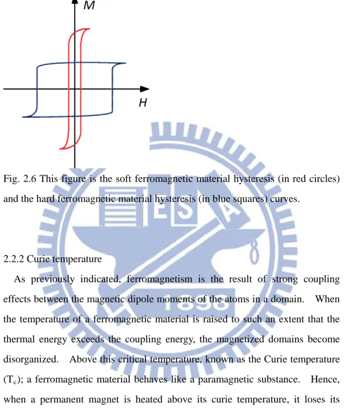
When an external magnetic field is applied to a ferromagnetic material, the walls of those domains having magnetic moments aligned with the applied field and which move in such a way as to make the volumes of those domains grow at the expense of other domains. As a result, magnetic flux density is increased. For weak applied fields, domain-wall movements are longer/ long acting reversible, and domain rotation toward the direction of the applied field will occur. For example, the M-H plane for Fe86V14 film is shown in Fig. 2.5, if an

16

applied field is reduced to zero at point P1, the M-H relationship will not follow

the red curve P2P1O, but will go down from P2 to P2’, along the lines of the

broken curve in the figure. This phenomenon of magnetization lagging behind the field producing it is called hysteresis. As the applied field becomes even much stronger (past P1 to P2), domain-wall motion and domain rotation will

cause essentially a total alignment of the microscopic magnetic moments with the applied field, at which point the magnetic material is said to have reached saturation Ms. The curve OP1P2

If the applied magnetic field is reduced to zero from the value at P

on the M-H plane is called the virgin magnetization curve.

2, the

magnetic magnetization does not reduce to zero but assumes the value at Mr

To make the magnetic magnetization of a specimen zero, it is necessary to apply magnetic field intensity H

. This value is called the residual or remanent magnetization (10 kOe =1 T) and is dependent on maximum applied field intensity. The existence of a remanent magnetization in a ferromagnetic material makes permanent magnets possible.

c in the opposite direction. This required Hc;

the coercive force; but a more appropriate name is coercive field intensity (in Oe). Like Mr, Hc also depends on the maximum value of the applied intensity.

17

Fig. 2.2 Domain structure of a polycrystalline specimen model[17].

Fig. 2.3 The Bitter method image, which was taken in a zero field and at room temperature, of the Fe81Ni19 array films in a completely demagnetized state.

18

Fig. 2.4 The Magnetic Force Microscopy (MFM) image, which was taken in a zero field and at room temperature, of the La0.7Sr0.3MnO3 (LSMO) films in a

completely demagnetized state.

Fig. 2.5 The virgin magnetization (in red circles) and the major hysteresis (in black squares) curves of the Fe86V14 film. 4πM is the magnetization of the

19

2.2.1 Soft magnetic materials and Hard magnetic materials

Ferromagnetic materials for use in electric generators, motors, and transformers should have a large magnetization for a very small applied field. As the applied magnetic field intensity varies periodically between + Hmax

Good permanent magnets, on the other hand, should show a high resistance to demagnetization. This requires that they are made with materials that have large coercive field intensities H

, the hysteresis loop is traced once per cycle. The area of the hysteresis loop corresponds to energy loss (hysteresis loss) per unit volume per cycle. Hysteresis loss is the energy lost in the form of heat in overcoming the friction encountered during domain-wall motion and domain rotation. Ferromagnetic materials, which have tall narrow hysteresis loops with small loop areas, are referred to as “soft” materials, there is shown in Fig. 2.6 red curve; they are usually well-annealed materials with very few dislocations and impurities so that the domain walls can move easily.

c and hence wider hysteresis curve, like the blue

curve in Fig. 2.6. These materials are referred to as “hard” ferromagnetic materials. The coercive field intensity of hard ferromagnetic materials can be 500 Oe or more, whereas that for soft materials is usually 50 Oe or less[2, 3, 16].

20

Fig. 2.6 This figure is the soft ferromagnetic material hysteresis (in red circles) and the hard ferromagnetic material hysteresis (in blue squares) curves.

2.2.2 Curie temperature

As previously indicated, ferromagnetism is the result of strong coupling effects between the magnetic dipole moments of the atoms in a domain. When the temperature of a ferromagnetic material is raised to such an extent that the thermal energy exceeds the coupling energy, the magnetized domains become disorganized. Above this critical temperature, known as the Curie temperature (Tc); a ferromagnetic material behaves like a paramagnetic substance. Hence,

when a permanent magnet is heated above its curie temperature, it loses its magnetization. The Curie temperature of most ferromagnetic materials lies between a few hundred to a thousand degrees Celsius, that of iron being 770°C[2, 3].

21

2.3 Magnetic anisotropy

The magnetization changes from zero to the saturation value, which the value of Ms

One factor which may strongly affect the shape of the M, H curve, or the shape of the hysteresis loop, is magnetic anisotropy. This term simply means that the magnetic properties depend on the direction in which they are measured. This general subject is of considerable practical interest, because anisotropy is exploited in the design of most magnetic materials of commercial importance. A thorough knowledge of anisotropy is thus important for an understanding of these magnetic materials[2, 3].

itself will be regarded simply as a constant of the material. If we understand the several factors that affect the shape of the M, H curve, we will then understand why some materials are magnetically soft and others are magnetically hard.

There are several kinds of anisotropy such as crystal anisotropy, shape anisotropy, stress anisotropy, and induced anisotropy.

2.3.1 Crystal anisotropy

The existence of crystalline anisotropy may be demonstrated by the magnetization curves of single-crystal specimens. By magnetization curve we mean the component of magnetization in direction of applied field M, plotted as a function of the applied field[16]. Magnetization curves for single crystals of iron, nickel, and cobalt for various orientations of the applied field with respect to the crystal axis for room temperature are shown in Fig. 2.7, Fig. 2.8, and Fig. 2.9. It is clear that much smaller fields are required to magnetize the crystals to

22

saturation along which the magnetization tends to lie are called easy axis (EA); the axis along which it is most difficult to produce saturation are called hard axis (HA).

Fig. 2.7 Magnetization curves of single-crystal of iron[16].

23

Fig. 2.9 Magnetization curves of single-crystal of cobalt[16].

2.3.2 Shape anisotropy

Consider a polycrystalline specimen having no preferred orientation of its grains, and therefore no net crystal anisotropy. If it is spherical in shape, the same applied field will magnetize it to the same extent in any direction. But if it is nonspherical, it will be easier to magnetize it along a long axis than along axis. The reason for this is the demagnetizing field along a short axis is stronger than along a long axis. The applied field along a short axis then has to be stronger to produce the same true field inside the specimen. Thus shape alone can be a source of magnetic anisotropy.

24

2.3.3 Stress anisotropy

The main reason for stress anisotropy is the inverse magnetostrictive effect, which will be discussed in section 2.4. Simply put, there exists an inverse effect which causes such properties as permeability and the size and shape of the hysteresis loop to be strongly dependent on stress in many materials. Magnetostriction therefore has many practical consequences, and a great deal of research has accordingly been devoted to it[2, 3, 16].

2.3.4 Induced anisotropy

Various other anisotropies may be induced in certain materials, chiefly solid solutions, by appropriate treatments. These induced anisotropies are of interest both to the physicist, for the light they throw on basic magnetic phenomena, and to the technologist, who may exploit them in the design of magnetic materials for specific applications[2, 3, 16].

The following treatments can induce magnetic anisotropy: (1) Magnetic annealing:

This mean heat treatment in a magnetic field, sometimes called a thermomagnetic treatment. This treatment can induce anisotropy in certain alloys.

(2) Stress annealing:

This means heat treatment of a material that is simultaneously subjected to an applied stress.

(3) Plastic deformation:

This can cause anisotropy both in solid solutions and in pure metals, but by quite different mechanisms.

25

This means irradiation with high-energy particles of a sample in a magnetic field.

26

2.4 Magnetostriction[2, 3]

When a ferromagnetic substance is exposed to a magnetic field, its dimensions change. This effect is called magnetostriction. It was discovered in 1842 by James Joule, who showed that an iron rod increased in length when it was magnetized lengthwise by a weak field. The fractional change in length ∆l/l is simply a strain, and, to distinguish it from the ε caused by an applied stress, we give the magnetically induced strain a special symbol λ[2, 3]:

λ =Δ𝑙_{𝑙 (2.10)}

The value of λ measured at magnetic saturation is called the saturation magnetostriction λs, and, when the word “magnetostriction” is used without

qualification, λs is usually meant. Magnetostriction occurs in all pure

substances. However, even in strongly magnetic substances, the effect is usually small: λs is typically of the order of 10

-5

The longitudinal, sometimes called Joule, magnetostriction just described is not the only magnetostrictive effect. Others include the magnetically induced torsion or bending of a rod. These effects, which are really only special cases of the longitudinal effect, will not be described here.

[3].

The value of the saturation longitudinal magnetostriction λs can be positive,

negative, or, in some alloys at some temperature, zero. The value of λ depends on the extent of magnetization and hence on the applied field, and Fig. 2.10 shows how λ typically varies with 𝐻��⃑ for a substance with positive

27

magnetostriction. As mentioned in the preceding, the process of magnetization occurs by two mechanisms, domain-wall motion and domain rotation. For example, the magnetostriction of an iron crystal dependence on magnetic field in the [100] direction is shown in Fig. 2.11.

Between the demagnetized state and saturation, the volume of a specimen remains very nearly constant. This means that there will be a transverse magnetostriction λt

λ_𝑡 = −1_{2 λ (2.11)}

very nearly equal to one-half the longitudinal magnetostriction and opposite in sign, or

When technical saturation is reached at any given temperature, in the sense that the specimen has been converted into a single domain magnetized in direction of field, further increase in field cause a small further strain. This causes a slow change in λ with H called forced magnetostriction, and the logarithmic scale of

H in Fig. 2.10 roughly indicates the fields required for this effect to become

appreciable. It is caused by the increase in the degree of spin order which very high fields can produce[3].

The longitudinal, forced-magnetostriction strain λ shown in Fig. 2.10 is a consequence of a small volume change, of the order of ∆V/V=10-10

per Oe, occurring at fields beyond saturation and called volume magnetostriction. It causes an equal expansion or contraction in all directions. Forced magnetostriction is a very small effect and has no bearing on the behavior of practical magnetic materials in ordinary fields[2, 3].

28

29

Fig. 2.11 indicates magnetostriction of an iron crystal in the [100] direction[3].

2.4.1 Measure λ on bulk or ribbon

The measurement of longitudinal magnetostriction is straightforward but not trivial, especially over a range of temperatures. While early investigators used mechanical and optical levers to magnify the magnetostrictive strain to an observable magnitude, today this measurement on bulk or ribbon samples is commonly made with an electrical-resistance strain gage cemented to the specimen. The gage is made from an alloy wire or foil grid, embedded in a

30

thin paper or polymer sheet, which is cemented to the sample. When the sample changes shape, so does the grid, and the change in shape also causes a change in the electrical resistance of the gage. With ordinary gages, the fractional change in resistance is about twice the elastic strain. This is typically a small resistance change, but one fairly easily measured with a bridge circuit, either ac or dc[3].

Fig. 2.12 Magnetostriction measurement on a sample (bulk or ribbon) using a strain gage[3].

31

2.4.2 Measure λ on thin film

Thin film samples present special challenges in the measurement of magnetostriction, since the films are almost always bonded to a nonmagnetic substrate. If the substrate is thin enough, a change in dimension of the film may produce a measurable curvature in the substrate, from which the magnetostrictive strain can be deduced. Another approach is to apply a known stress to the sample and measure the resulting change in magnetic anisotropy. This method demonstrates the concept of the stress anisotropy.

32

2.5 Ferromagnetic Resonance

Spin resonance in ferromagnetic metals, called simply ferromagnetic resonance, is complicated by eddy-current effects. At frequencies of about 1010

If the applied field is not large enough to saturate a ferromagnetic sample, resonance phenomena may still occur. Various nonuniform resonance modes may arise, by which different parts of the sample are magnetized in slightly different directions, each oscillating in resonance. There can also be domain wall resonance associated with small-scale oscillatory motion of domain walls. Many of these phenomena are discussed by C. Kittel[2, 16].

Hz, eddy-current shielding of the interior of the specimen is so nearly complete that the depth of penetration of the alternating field is only about 100 nm or 300 atom diameters. (Skin effect will be discussed in next section.) The specimen is therefore usually composed of powder particles of about this diameter, or of a thin film.

Energy losses at resonance frequencies, by which the oscillatory motion of the electron spins is converted to heat in the sample, determine the width of the resonance peak, the peaks in insulating samples can be very narrow: less than 1 Oe. In metals the peaks may be 1000 times broader[16]. The energy losses also control the speed with which a ferromagnetic material can reverse its direction of magnetization.

If there are no losses at all, or zero damping in the usual terminology, then the magnetization only precesses around the applied field and never becomes parallel to the field. And if damping is very large, the magnetization approaches the field direction very slowly, and switching time is hopelessly slow.

33

An intermediate level of losses, called critical damping, leads to the fastest switching[2, 16].

Curiously, the form of the equation that describes the damping is not obvious. If the damping is small compared to the precession, a formulation called the Landau-Lifshitz equation was proposed as early as 1935[3, 16]:

𝜕𝑀��⃑

𝜕𝑡 = −γ�𝑀��⃑ × 𝐻��⃑� − λ 𝑀

��⃑ × �𝑀��⃑ × 𝐻��⃑�

𝑀2 (2.12)

The first term is the precession motion, and the second term is the damping, with λ as an adjustable damping parameter. The constant γ = ge/2mec, where e and

me

An alternative damping term was proposed by Gilbert, namely

are the charge and mass of electron, c is the velocity of light, and g is the g-factor (=2 for electron spin), respectively.

−_{𝑀 �𝑀}𝛼 ��⃑ × 𝑑𝑀_{𝑑𝑡 � ,}��⃑ where α = 𝑀��⃑ × �𝑀_𝑀��⃑ × 𝐻��⃑�₂

Ref. [16] shows that the Landau-Lifshitz equation can be written in the form

𝜕𝑀��⃑

𝜕𝑡 = −γ�𝑀��⃑ × 𝐻��⃑� + 𝛼𝑀 �𝑀��⃑ × 𝑑𝑀 ��⃑

𝑑𝑡 � + γ𝛼2�𝑀��⃑ × 𝐻��⃑�. (2.13)

If α is small, the term is negligible and equation 2.13 becomes the Gilbert equation. The full form of equation 2.13 can be called Landau-Lifshitz-Gilbert equation (LLG equation), as

34

𝜕𝑀��⃑

𝜕𝑡 = −γ�𝑀��⃑ × 𝐻��⃑� + 𝛼𝑀 �𝑀��⃑ × 𝑑𝑀 ��⃑

35

2.6 Skin effect

In high-frequency applications, the current in a good conductor tends to shift to the surface of the conductor, resulting in an uneven current distribution in the inner conductor and thereby changing the value of the internal inductances. In the extreme case, the current may essentially concentrate in the “skin” of the inner conductor as a surface current, and the internal self-inductance is reduced to zero.

Then a high-frequency electromagnetic wave is attenuated very rapidly as it propagates in a good conductor. The distance δ through which the amplitude of traveling plane wave decreases by factor of e-1 (= 0.368) is called the skin depth of a conductor

[17]

:

δ = ( 𝜌

𝜋𝜇𝑓)1/2 (2.15)

Where ρ is resistivity, f is microwave frequency, µ is permeability.

At microwave frequencies, the skin depth of penetration of a good conductor is so small that fields and currents can be confined in a very thin layer of the conductor surface. For example, at 10 GHz it is a very small distance 0.66 µm for copper

[17]

.

36

3. Experiments

3.1 Process

3.1.1 Samples for film

This is the flow chart of the experimental process. We checked the film thickness by Dektak3. The film’s structure was shown in the X-ray diffraction data. The Young’s modulus of each film was obtained from the nano-indentation system. The magnetization hysteresis was measured by VSM system. Our main experiments are the magnetostriction hysteresis and FMR measurements.

Sample Preparations

Dektak3

XRD

Nano-Indentation

VSM

37

3.1.2 Samples for ribbon

This is the flow chart of the experimental process. We checked the ribbon thickness by vernier. The ribbon’s structure was shown in the X-ray diffraction data. The resistivity of each film was obtained from the van der Pauw method. The magnetization hysteresis was measured by VSM system. Our main experiments are the magnetostriction hysteresis measurements.

Sample Preparations

Thickness

XRD

_VSM

Resistivity

38

3.2 DC magnetron sputtering method

DC magnetron sputtering is a physical rather than a chemical or thermal process in making films in making films. Permanent magnets are used in the sputtering gun in order to shorten the ionization mfp for the displaced atoms that fly randomly inside the vacuum chamber. Then atoms are physically ejected from a target material by high-energy gas ions, usually argon ions[19, 20]. The arrangement is shown in Fig. 3.1. It is necessary to create plasma of ionized gas in the deposition chamber. The presence of stable plasma, created by the gas atoms, is a necessary[3].

The advantages of dc magnetron sputtering are[21]: 1. Multicomponent films can be deposited.

2. Refractor materials can be deposited. 3. Insulating films can be deposited. 4. Good film adhesion is assured.

5. Low-temperature epitaxy is possible.

6. Thickness uniformity over lager planar areas can be obtained.

The disadvantages are:

39

Fig. 3.1 Thin film prepared by dc magnetron sputtering.

3.2.1 Process conditions

A series of magnetic thin films, Fe81-xNixGa19/Si(100) and

Fe81-yNiyGa19/glass films, with x, y = 0, 4, 7, 11, 17, 22,and 26 at. % Ni, were

deposited films by alloy targets and the dc magnetron sputtering method. The dc magnetron sputtering system is shown in Fig. 3.2, and the working conditions are listed as following:

40

1. The working gas (99.999% argon) pressure was 5 mTorr. 2. The sputtering power were 80W

3. The deposition temperature (TS) was at room temperature (RT). 4. The film thickness was 1000 Å.

41

3.3 Rapid quenching melt-spun method

A series of magnetic metallic ribbons, Fe81-zNizGa19 with z  = 0, 3, 7, 13,

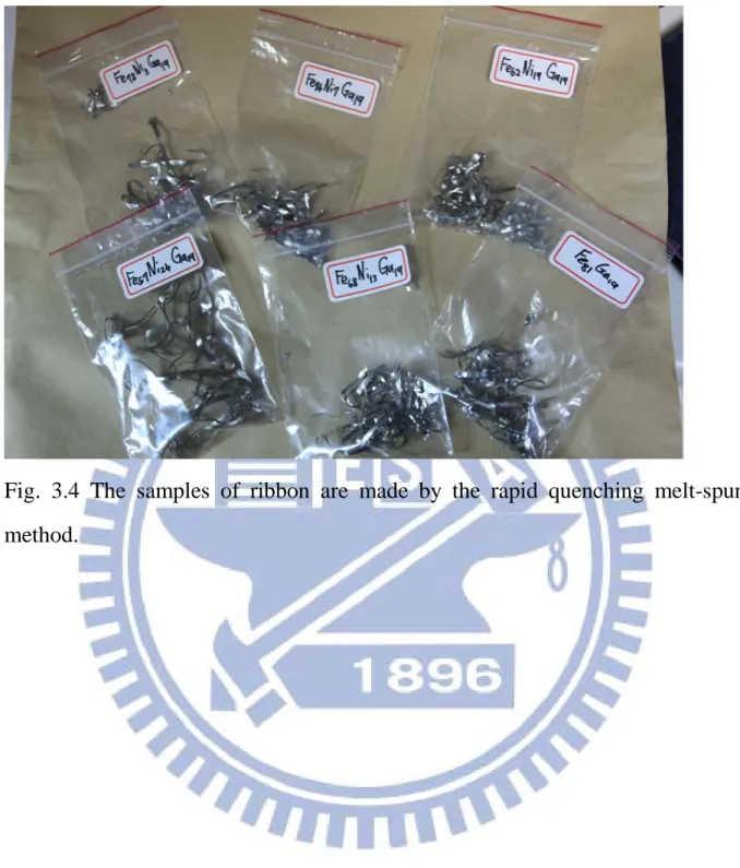
and 24, were made by the rapid quenching melt-spun method in a low vacuum chamber, the arrangement is shown in Fig. 3.3[3, 22]. The surface velocity of the rotating copper wheel was about 15m/s. The average thickness (t) of the ribbon is about 0.03 mm and the width (w) is about 4mm, which is shown in Fig. 3.4.

42

Fig. 3.4 The samples of ribbon are made by the rapid quenching melt-spun method.

43

3.4 The Dektak

3

system

The Dektak3 system is a high precision measuring system which accurately measures surface texture, shown in the Fig. 3.5. Table 3.1 is the technical specifications for Dektak3 system.

3.4.1 Principle of operation

There is the mobile diamond-tipped stylus on Dektak 3 to measure the surface texture of the sample. The high precision stage moves a sample beneath the stylus according to a programmed scan length and speed. The stylus on the stage is mechanically coupled to the core of a linear variable differential transformer (LVDT). As the stage moves the stylus on the sample, the stylus rides over the sample surface. The stylus is translated vertically on the surface variations. The information with electrical signals depending on the stylus movement is produced as the core position of the LVDT changes respectively. An analog signal proportional to the position change is produced by the LVDT, which in turn is conditioned and converted to a digital format through a high precision, integrating analog to digital converter. The results of the digitized signals from a single scan are stored in computer memory for display, manipulation, and measurement, the process figure is shown in Fig. 3.6[23].

44

Fig. 3.5 shows Dektak3 system

[23]

.

Table 3.1 Technical specifications

[23]

Vertical data resolution 5 Å maximum Vertical range 65.5 μm maximum Scan length range 50 μm to 30 mm

45

46

3.5 X-ray diffraction (XRD)

Fig. 3.7 shows the incoming beam let each scatterer to re-radiate a small portion of its intensity as a wave. Then scatterers are arranged symmetrically with distance d, these waves will be in sync (add constructively) only in directions where their path-length difference 2dsinθ=nλ, called Bragg's law[26].

In this study, the structural properties were characterized by the X-ray diffraction (XRD) using CuKα1 line (λ = 1.5405 Å). There are shown typical x-ray diffraction patterns in Fig. 3.8 and Fig. 3.9, and other results are shown in chapter 7 appendix.

47

Fig. 3.8 The X-ray diffraction figure on series of Fe81-yNiyGa19/glass films.

48

3.6 Nano-indentation system measure

The Young′s modulus (E f) of the each film was obtained from the

nano-indentation system, which is shown in Fig. 3.10. From each indentation cycle, the depth of circle of contact (hp) is obtained. For details of the hp

measurement, please refer to Ref. [24]. From a series of indenting tests (i.e., from heavy to light loadings) we can plot the measured E as a function of hp.

Usually, Ef is taken in the hp range, where hp = tf /15 to tf

E = Es + (Ef− Es)e− hp

t∗ _{, (3.1)}

/10. Alternatively, the following empirical equation is used for fitting [25, 27]:

where ES is the Young′s modulus of the substrate, and t* is a fitting parameter.

The solid curves in Fig. 3.11 show the best-fit results, by using Eq. 3.1, for all the Fe81-yNiyGa19/glass films. When hp > 0.05 µm in Fig. 3.11, E tends to

approach a fixed value, i.e., ES ≅ 76 GPa [8], of the 0211 Corning glass

substrate. The E vs. hp fitting plots for the Fe81-xNixGa19/Si(100) films look

similar to Fig. 3.11, except that all the plots are shifted upward, with ES ≅ 130

49

Fig. 3.10

Nano-indentation system.

Fig. 3.11 Solid curves represent the best-fit results of E vs. hP, where E is the

Young′s modulus and hp is the depth of circle of contact, obtained from

50

3.7 Electrical resistivity measurement

In this study, we measured the electrical resistivity (ρ) by the collinear

four-probe array, which is shown in Fig. 3.12. ρ is calculated by the equation as, ρ = 1 2 × (𝑉+− 𝑉−) 𝐼 × 𝑡𝑊 𝐿 × C (3.2)

where V+ means V2-V1 for +I, V- means V2-V1 for -I, ρ is in unit of µΩ-cm, and

C is a correction factor, dependent on both the ratios W/L and /W[28]. Table 3.2 shows the calculated dependence of the correction factor C on W/L and /W. In our case, C≒1.

51

Table 3.2 Correction factor C for the calculation of the resistivity measured with collinear four-point probes placed on a symmetry axis[28].

W/L Circle Square Rectangle Rectangle Rectangle

C for dia. d C for /W=1 C for /W=2 C for /W=3 C for /W=4

1.0 0.9988 0.9994 1.5 1.4788 1.4893 1.4893 2.0 1.9454 1.9475 1.9475 3.0 2.2662 2.4575 2.7000 2.7005 2.7005 4.0 2.98289 3.1137 3.2246 3.2248 3.2248 5.0 3.3625 3.5098 3.5749 3.5750 3.5750 10.0 4.1716 4.2209 4.2357 4.2357 4.2357 20.0 4.4364 4.4516 4.4553 4.4553 4.4553 ∞ 4.5324 4.5324 4.5324 4.5324 4.5324

52

3.8 Ferromagnetic resonance (FMR) experiments

The cavity used was a Bruker ER41025ST X-band resonator which was tuned at fR = 9.6 GHz. The films were oriented such that EA//H��⃑𝑧 and EA⊥h�⃑rf.

The EA means easy-axis. Where H��⃑_𝑧 was an in-plane external field, which varied from 0 to 2 kOe, and h�⃑_rf was the microwave field, ω is angle velocity for z-axis, and z-axis is EA of the film. Configuration is depicted schematically in Fig. 3.13. A typical FMR absorption spectrum of the Fe59Ni22Ga19/glass film

is shown in Fig. 3.14, where we can spot an FMR event manifested by an absorption peak at H = HR and define the half-peak width (∆H)exp. In this case,

HR = 671.4 Oe and (∆H)exp = 133.9 Oe were obtained[29].

53

0

500

1000

1500

2000

0.02

0.04

0.06

0.08

0.10

0.12

Fe

₅₉

Ni

₂₂

Ga

₁₉

/glass 100nm

H

_R

=671.4 Oe

H (Oe)

EA//H

(

∆H

)

_exp

=133.90 Oe

Ins

tens

ity

Fig. 3.14 A typical FMR absorption spectrum of the Fe59Ni22Ga19/Glass film at

54

3.9 Vibrating-Sample Magnetometer (VSM)

Fig. 3.15 shows the vibrating sample magnetometer used for measuring the magnetization as a function of applied field. It is based on the flux change in a coil when a magnetized sample is vibrating nearby. The sample, commonly a small disk, is attached to the end of a nonmagnetic rod, the other end of which is fixed to a loudspeaker cone or to some other kind of mechanical vibrator. The oscillating magnetic field of the moving sample induces an alternating emf in detection coils, whose magnitude is proportional to the magnetic moment of the sample. The alternating emf is amplified, usually with a lock-in amplifier which is sensitive only to signals at the vibration frequency. The lock-in amplifier must be provided with a reference signal at the frequency of vibration, which can come from an optical, magnetic, or capacitive sensor coupled to the driving system. The detection-coil arrangement usually involves balanced pairs of coils to cancel signals due to variations in the applied field. The apparatus is calibrated with a specimen of known magnetic moment, which must be of the same size and shape as that of the sample to be measured, and should also be of similar permeability[3].

The driving system may be mechanical, through a cam or crank and a small synchronous motor, or in a recent commercial instrument, with a linear motor. In our case, shown in Fig. 3.16, the vibration frequency is generally below 85 Hz, and the vibration amplitude is a few millimeters. The amplitude is fixed by the geometry of the mechanical system or by the drive signal delivered to the linear motor. The amplitude may vary, depending on the mass of the sample and/or the frequency of vibration. One method is to and a second set of

55

sensing coils. Then the signal from these coils can be used in the feedback loop to maintain constant amplitude of vibration. Alternatively, a portion of the signal from the permanent magnet can be balanced against the signal from the unknown sample, making the method a null method[30].

Extreme care is necessary to minimize vibration of the sensing coils in the field, and to prevent the measuring field from influencing other parts of the system. Note that the VSM measures the magnetic moment m of the sample, and therefore the magnetization M can be obtained.

56

Fig. 3.16 Vibrating-Sample Magnetometer (VSM). Courtesy Lake Shore Cryotronics, Inc.

3.9.1 Measuring hysteresis loops

The field-in-plane magnetic hysteresis loops were obtained by varying sample orientation with respect to the applied field in the vibrating sample magnetometer (VSM) measurements to indentity the easy-axis (EA) and hard-axis(HA)[29]. When the squareness ratio (SQR ≡Mr/MS) is the largest,

the corresponding orientation is defined the EA. Similarly, the orientation with the smallest SQR is identified as the HA. A typical example is shown in Fig. 3.17. In most cases, the angular dependence of SQR is roughly sinusoidal with a period of 180°. For the more, the HA hysteresis loop of the