週選擇權上市對台灣選擇權市場流動性之衝擊探討

(1)

國立交通大學

資訊管理與財務金融學系

財務金融碩士班

碩士論文

週選擇權上市對台灣選擇權市場流動性之衝擊探討

Impacts of Introducing Weekly Options on the Liquidity of

Option Market in Taiwan

研究生：周承儀

指導教授：鍾惠民教授

周幼珍教授

(2)

Impacts of Introducing Weekly Options on the Liquidity of

Option Market in Taiwan

研究生：周承儀

Student：Cheng-Yi Chou

指導教授：鍾惠民、周幼珍 Advisor：Huimin Chung

Yow-Jen Jou

國立交通大學

資訊管理與財務金融學系

財務金融碩士班

碩士論文初稿

A Thesis

Submitted to Graduate Program of Finance Department of Information Management and Finance

National Chiao Tung University

in partial Fulfillment of the Requirements for the Degree of

Master of Science In Finance July, 2014 Hsinchu, Taiwan

中華民國一百零三年七月

(3)

週選擇權上市對台灣選擇權市場流動性之衝擊探討

學生：周承儀指導教授：鍾惠民教授周幼珍教授

國立交通大學資訊管理與財務金融學系財務金融碩士班

中文摘要

本篇論文主要探討台灣選擇權市場在週選擇權上市交易後，對月選擇權市場成交量、流動性、以及標的市場價格波動造成的衝擊，本文使用聯立迴歸方程式分析月選擇權市場交易量、流動性及標的市場價格波動。其結果指出，週選擇權上市對於月選擇權成交量以及流動性有顯著的降低作用。同時，結果也顯示週選擇權上市具有穩定標的市場價格波動的效果。此外，本文亦分析週選擇權上市對於月選擇權市場成交量、流動性、以及標的市場價格波動在到期日當週造成之衝擊，以及檢驗週選擇權上市對不同價內外程度選擇權的衝擊變化，其結果顯示週選擇權上市對於到期日前月選擇權交易並無明顯的影響，且選擇權交易量仍具有明顯的到期日效應；在區分價內外後，也可發現週選擇權上市對於價平選擇權的成交量影響較為明顯。相反的，其對於流動性的影響則在價內外選擇權較為明顯。至於價格波動則無明顯的差別。關鍵字：週選擇權上市、流動性、月選擇權、價格波動 I

(4)

Impacts of Introducing Weekly Options on the Liquidity of

Option Market in Taiwan

Student: Cheng-Yi Chou Advisor:Prof.Huimin Chung

Prof. Yow-Jen Jou

Graduate Program of Finance

Department of Information Management and Finance

National Chiao Tung University

Abstract

This paper aims to examine the impacts of introducing weekly option on the volume and liquidity of monthly options, and the stability of the underlyingmarket. Our study applies a simultaneous equation approach to analyze the trade volume and liquidity of monthly option market, and the price volatility of the underlying market. The results show that introducing weekly option reduces the volume and liquidity of options, while stabilizing the underlying market. In addition, we examine the impactsof weekly option listing on volume, liquidity, and underlying market volatilitynear settlement days and by option moneyness, respectively. . Results show that the introduction of weekly options has no additional impacton monthly options near settlement days, while the expiration day effects on trade volume still exist. Besides, the impacts of weekly option listing on volume are significant onlyfor the at-the-money options, while the impacts on liquidity are significant on the in-the-money and out-of-the-money options. However, as for price volatility of underlying market, there are no obvious differences between options with different moneyness.

Keywords: Weekly option listing, liquidity, monthly option, price volatility

(5)

Acknowledgments

謹此致謝曾在此篇論文上協助過我的所有人，特別是鍾惠民教授、周幼珍教授、邱敬貿學長、陳清和學長不厭其煩得指導，以及口試委員謝文良教授的指導與建議，才得以順利完成此篇論文。在說長不長、說短不短的兩年多研究所生涯中，除感謝許多老師用心的教導外，也非常感謝有一群同甘共苦的同學一起度過這段時光。在遇到困難的時候一起訴苦的袋鼠、一起努力準備甄試的蘇瑞與珮甄、給了許多增廣見聞見識的狗狗、幽默數學大師雞皮、人人稱羨的小銘與憶慈等，族繁不及備載，雖然並不一定在論文上有直接的幫助，但間接的在心裡建設上也有多少作用，在此一併感謝。最重要的還是最感謝父母在家境困頓的情況下讓我盡量無虞的順利完成這兩年的學業，雖然只有短短一行字，其中包含了最大量的感謝與尊敬。另外也要感謝李怡樺學姊在這兩年中給我機會一起做了報告，在其中學習到不少在學校沒注意過的事情，也有機會可以將所學真正派上用場。若有此篇闕漏的被感謝人，在此一併致上最真誠的謝意。

Wish all of you have love & peace

承儀 2014/10/16 於交大竹湖

(6)

Figures and Tables

FIGURE I:DAILY TRADED VOLUMES OF MONTHLY AND WEEKLY OPTIONS. ... 12

TABLE I:SUMMARY STATISTICS ... 13

TABLE II:CORRELATIONS BETWEEN INDEPENDENT VARIABLES ... 14

TABLE III:IMPACTS OF INTRODUCING WEEKLY OPTIONS ON MONTHLY OPTIONS ... 16

TABLE IV:IMPACTS OF INTRODUCING WEEKLY OPTIONS ON MONTHLY OPTIONS NEAR EXPIRATION DAYS AND THE EXPIRATION DAY EFFECT ... 18

TABLE V:COEFFICIENTS OF DUMMY VARIABLES OF MODEL (2) ... 19

TABLE VII:IMPACTS OF INTRODUCING WEEKLY OPTIONS ON MONTHLY OPTIONS AFTER THE ADJUSTMENT ON LIQUIDITY ... 23

TABLE VIII:IMPACTS OF INTRODUCING WEEKLY OPTIONS ON MONTHLY OPTIONS NEAR EXPIRATION DAYS AND THE EXPIRATION DAY EFFECT AFTER THE ADJUSTMENT ON LIQUIDITY ... 24

TABLE IX:IMPACTS OF INTRODUCING WEEKLY OPTIONS ON MONTHLY OPTIONS ... 29

TABLE X:IMPACTS OF INTRODUCING WEEKLY OPTIONS ON MONTHLY OPTIONS NEAR EXPIRATION DAYS AND THE EXPIRATION DAY EFFECT (AT-THE-MONEY CALL OPTIONS) ... 30

TABLE XI:IMPACTS OF INTRODUCING WEEKLY OPTIONS ON MONTHLY OPTIONS ... 31

TABLE XII:IMPACTS OF INTRODUCING WEEKLY OPTIONS ON MONTHLY OPTIONS NEAR EXPIRATION DAYS AND THE EXPIRATION DAY EFFECT (AT-THE-MONEY PUT OPTIONS) ... 32

TABLE XIII:IMPACTS OF INTRODUCING WEEKLY OPTIONS ON MONTHLY OPTIONS ... 33

TABLE XIV:IMPACTS OF INTRODUCING WEEKLY OPTIONS ON MONTHLY OPTIONS NEAR EXPIRATION DAYS AND THE EXPIRATION DAY EFFECT (IN-THE-MONEY CALL OPTIONS) ... 34

TABLE XV:IMPACTS OF INTRODUCING WEEKLY OPTIONS ON MONTHLY OPTIONS ... 35

TABLE XVI:IMPACTS OF INTRODUCING WEEKLY OPTIONS ON MONTHLY OPTIONS NEAR EXPIRATION DAYS AND THE EXPIRATION DAY EFFECT (IN-THE-MONEY PUT OPTIONS) ... 36

(8)

TABLE XVII:IMPACTS OF INTRODUCING WEEKLY OPTIONS ON MONTHLY OPTIONS ... 37 TABLE XVIII:IMPACTS OF INTRODUCING WEEKLY OPTIONS ON MONTHLY OPTIONS NEAR

EXPIRATION DAYS AND THE EXPIRATION DAY EFFECT (OUT-OF-THE-MONEY CALL OPTIONS) ... 38

(9)

1 Introduction

Weekly options are popular among exchanges worldwide recently. Starting from 2005, CBOE first introduced weekly options. NYSE Euronext, CME, and ICE also launched weekly options in 2006, 2011, and 2012 respectively. Thestrong growth for short maturity optionsin financial markets suggests that different kinds of short maturity options, such as weekly and daily options, are gradually accepted by investors around the world.For example, as CBOE decided to expand interest in weekly options in 2010, the trade volume grew from 1% of total volume to about 15%, which the average daily volume grew from less than 25,000 contracts to about 100,000 contracts in 2012. Furthermore, the types of underlying assets also expanded. There were only a handful of weekly options of ETFs and individual stocks in 2010, while six

indexes, 26 ETPs and 119 individual stocks in 2012.1In Taiwan, weekly options were

introduced on Nov 2012.According toChinese National Futures Association, the average daily volume of weekly options, from the introduction to Mar 2013, accounts for 40.29% of the volume of TXO market. In addition, based on the statistics of Taiwan Futures Exchange,the volume of TXO market increased by 25%from the listing of weekly options to Feb 2013.

Prior studies document that introducing option affects the volatility of underlying assets through hedging transactions. For instance,Bansal, Pruitt, and Wei (1989) suggest that option listing in CBOE market leads to a decrease in the total (but not systematic) risk of theunderlyingfirms.Chen and Chang (2008) find that stock options listing in Taiwan decreases the degree of volatility. In contrast, Wei, Poon, and Zee (1997) find an increase in volatility for a sample of 144 OTC stocks after option listing.

In addition, introducing weekly options islikely to impact the volume and liquidity of monthly options.In practice, weekly options are less expensive than monthly options with the

1_{The information related to weekly options are obtained from CBOE Weeklys splash page.}

1

(10)

nature of its high leverage. Also, the weekly options have the characteristics of rapid decrease of its time value and short duration. Consequently, investors using weekly options be able to tradetheir strategies more flexible than monthly options and hedge their portfoliosby using less costs. For example, option sellers may favor the use of weekly options because they take a lower risk due to the inherit characteristics ofweekly options,rapid decrease of its time value and short duration. However, investors are likely to use weekly options instead of some positions in their portfolios originally established by monthly options.This may subsequently impacts on the trade volume and liquidity of monthly options.

Despite the trades of weekly options have become popular, much less is known about the impact of its introduction on the volume and liquidity of monthly options, and the volatility of its underlying asset. The current study attempts to fill this gap.Because it is the first time to introduce short term derivativesin Taiwan, the results of the impact of weekly options onmonthly option marketand spot market may therefore be a referencefor TAIFEX to introduce other short maturity derivatives.

Another application of weekly options is strongly related to theexpiration day effects which cause abnormal trade volume and price swing duringsettlement. Chow et al. (2012) showed the expiration day effects of index futures on the cash market.Chow, Yung, and Zhang(2003)also showed the expiration day effects, a negative price effect and some return volatility, of Hang Seng Index (HSI) derivative market in Hong Kong. In order to benefit from these high volumes more frequently, stock exchanges offer short maturity derivatives.As options settled weekly, expiration day effects occur every week and traders cantake advantage of these volumes.

Prior literature has examined the impacts of introducing new derivatives on the existing markets.Kumar, Sarin, and Shastri(1995, 1998), find that option trading has some impacts on market qualities of underlying securities.Wang, Chung, and Yang (2007), based on the analysis of liquidity, suggest that the introducing E-mini futures hassignificant impact on the

(11)

transaction prices of regular index futures, market depth deterioration, and the increase in the bid-ask spread.Chen and Chung (2011) show that the introduction of SPDR options improves the liquidity of SPDRs and reduces implicit trading costs. Liu (2007) also tests the impacts of index options on liquidity and volatility of the S&P 100 market.

This paper aims to examine the impacts of introducing weekly options on the liquidity of monthly option markets, and the price volatility of the underlying market in Taiwan.Our results help policy makers understandwhether and when to launch other short maturity derivatives in Taiwan. The primary derivativebeing researched is the TXO index option traded at the Taiwan Futures Exchange.On one hand, we focus on the impact on the trade volume and liquidity of monthly options to see whether weekly options listingimprove the liquidity of monthly options.

Since, in practice, weekly options, monthly options, and the underlying asset are traded simultaneously, we follow the simultaneous equation model (SEM)of Wang, Chung, and Yang’s (2000) with an adjustment of two dummy variables to analyze the impacts of weekly options listing on the trade volume and liquidity of monthly options and the impacts near settlement.

Our study seeks to contribute to the empirical literature of option market in Taiwan. To the best of our knowledge, this is the first empirical research to examine how weekly options affect the liquidity of monthly options in Taiwan.Many research are about the impacts of introducing derivatives on the spot market. The results suggest that introducing weekly option significantly decreases the liquidity andvolume of monthly options. This is different from other research because this paper studies the impacts on monthly options, not the whole index option market. Moreover, the price volatility of the underlying market was reduced, indicating that the introduction of weekly options stabilizes the underlying market. This isidentical to similar research in other markets.For instance, Liu (2007) showed that S&P100 stock index options can stabilize its underlying market. In addition, we adjust the raw series data of

(12)

liquidity due possible common regularities and time trends and re-perform the SEM model. The effects of introducing weekly option still remain same.

The later parts of this paper are arranged as follows. Section 2 reviews literature about the impacts of introducing new derivatives and expiration day effects, and also gives hypotheses in this study. Section 3 describes details of data, data sources, and methodology. Section 4 shows the empirical results of the simultaneous equations.Section 5 is the robustness analysis. Section 6 gives the conclusion of this study and suggests the future research directions.

2 Literature Review

Although many empirical studies have examined the impacts of introducing new derivatives on the underlying market, the results are still inconclusive. On one hand, some studies support the view that introducing new derivatives would help improve the liquidity and stability of the underlying assets. Chatrath, Kamath, Chakornpipat andRamchander (1995), and Liu (2007) both find that S&P100 stock index options trading have stabilized and improve the liquidity of the underlying stock market. The listing of the S&P100 options results inhigher liquidity and lower volatility. Liu also notice that the index derivativelisting induces informed and speculative traders to migrate from the underlying market to the derivative market. Kumar et al. (1995) find that volatility and bid-ask spread decline for the stocks contained in the Nikkei 225 Index after thelisting of the index options.Specifically, after using cross-sectional regressions controlling for variations in volume, spread, and price, option listing is associated with the decrease in volatility for index stocks. Pilar& Rafael (2002) show that due to the introduction of futures and options, the conditional volatility of the underlying index declines. They also find that the trade volume of Ibex-35 also increases significantly in the Spanish market. Shenbagaraman(2003) suggest that index futures and

(13)

options listing not only improves the liquidity and reduces information asymmetry, but also find there is no evidence of any connection between trading activity in derivative market and spot market volatility. Chen and Chung (2011) show that the introduction of SPDR options improves the liquidity of SPDRs and reduces implicit trading costs. It also leads to a significant improvement of information shares of SPDRs.

On the other hand, Jegadeeshand Subrahmanyam(1993) find a higher spread and volatility of its underlying assets,controlling for changes in other spread determinants, after the listing of S&P 500 futures. Lamoureux andPannikath (1994), Freund, McCann and Webb (1994) and Bollen(1998) find that the impact of index options listings on volatility is not consistent over time. Wei, Poon and Zee (1997) findboth volume and price volatility increase for options on OTC marketfor a sample of 144 stocks in the USA.Price volatility still increase even controlling for volume, insider trading, andspreads.The evidence of spreads is mixed in their sample.Hason and Chowdhury (2011) also note that the effects of the introduction of index options are different in Asian stock markets. Only selected stock markets have an increase in their stock return volatility and liquidity.

Weekly options provide additional room, other than monthly index options, for speculators, hedgers, and informed traders so that they can migrate from stock option market to index option market. As suggested by Kumar et al.(1995), the increase in liquidity trading might not offset the decrease in speculative and informed trading after option listing, causing the decrease in trading volume. Moreover, this migration of volume also means that information asymmetry would lessen in the underlying market so that spread and volatility might decrease. Therefore, this study anticipates that introducing weekly options would decrease the volume and liquidity of monthly options, and the price volatility of the spot market because the speculative and hedging trading activities might decrease in the spot market.

The idea of short maturity option is also strongly related to the expiration day effect

(14)

which is proposed by Stoll and Whaley (1987, 1990, 1991) who argued that many arbitrageurs liquidate their holdings of underlying stocks at the same time as the expiration of the index futures and options contracts, causing large price swings and abnormal trading volumes. The model developed by Kumar and Seppi (1992) suggests that traders are incentivized to establish futures positions and then trade in the spot market to manipulate the prices of the underlying constituent stocks in order to accrue profits around the expiration day.Chung and Hseu (2008) show that there are significant price reversal, volatility and abnormal volume stemming from the expiration of MSCI-TW futures market. Chou et al. (2012) suggests that both volatility and trading volume are higher on the final settlement days in Taiwan.

Above all, the first hypothesis in this study is that the introduction of weekly options would take over the volume of monthly options, causing a decrease in its volume.Alike some previous empirical studies, the introduction of new derivatives usually results in a lower traded volume of the underlying securities. This study expect that weekly option listing would have those hedgers, speculators, and some certain traders transfer part of their positions in monthly options to weekly options and therefore decrease the volume of monthly options.The second hypothesis is that there would be a decrease in the liquidity of monthly options because of the decrease in the volume. Although the traded volume of monthly options decreases, the variation of bid-ask spread is still uncertain. In general, as volume of an security decrease, its bid-ask spread would broaden, which results in worse liquidity.The third hypothesis isthe price volatility of the underlying security would decrease due to the decrease in information asymmetry. In an imperfect market, the lower transaction costs and greater leverage of options market might attract more informed traders and then make the market become more informational efficient (e.g. Ross (1977), Grossman (1988)). The forth hypothesis is that these impacts might be not apparent near settlement days because the expiration day effects on monthly and weekly options would somewhat overlapped with the impacts. The abnormal volume and price swing during settlement periods make it hard to

(15)

distinguish between the impacts of weekly option listing and the expiration day effects. Therefore, it is anticipated that the impacts of weekly options would not be apparent near settlement days

3 Data & Methodology

The primary sources of the data are Taiwan Futures Exchange, and Taiwan Economic Journal Plus Database (TEL+ Database). Taiwan Futures Exchange database contains historical trading data of all futures and options traded in Taiwan. TEJ+ database provides complete trading data of indices in Taiwan.We use daily traded data of TXO index options from Taiwan Futures Exchange’s website and the period is between Dec 2011 and Dec 2013 which is one year before and after weekly option listing. Besides, we also take daily data of Taiwan Stock Exchange Capitalization Weighted Stock Index (TAIEX), mainly traded prices, to calculate historical volatility. Finally, the interest rates are obtained from TEJ+ database using Interbank Overnight Call-Loan Rate. We know that short-term interest rates will affect the cost of carrying of spot positions. Futures and options play an important role in hedging. As the cost of carrying in spot positions become higher, the hedging needs and speculative trading reduce simultaneously. As a result, futures and options trading volumes will decrease.

1. Data

Liquidity Measure (LIQ)

Since option data reveals a panel nature which makes the dollar bid-ask spread to be a liquidity measure. This paper uses the proportional bid-ask spread proposed by Chordia, Roll and Subrahmanyam(2000)(CRS hereafter) as our liquidity measure,noted 𝐿𝐿𝐿𝐿𝐿𝐿_𝑡𝑡:

𝑳𝑳𝑳𝑳𝑳𝑳

𝒕𝒕

=

∑

𝒂𝒂𝒊𝒊=𝟏𝟏

𝑽𝑽𝑽𝑽𝑳𝑳

𝒊𝒊_{(𝒂𝒂𝒂𝒂𝒂𝒂}𝒂𝒂𝒂𝒂𝒂𝒂_𝒊𝒊_{+𝒃𝒃𝒊𝒊𝒃𝒃}𝒊𝒊−𝒃𝒃𝒊𝒊𝒃𝒃_𝒊𝒊_)/𝟐𝟐𝒊𝒊

∑

𝒂𝒂𝒊𝒊=𝟏𝟏

𝑽𝑽𝑽𝑽𝑳𝑳

𝒊𝒊

where 𝑉𝑉𝑉𝑉𝐿𝐿_𝑖𝑖 is the volume of option𝑖𝑖, 𝑎𝑎𝑎𝑎𝑎𝑎_𝑖𝑖 is the responding best ask price in one

(16)

day,𝑏𝑏𝑖𝑖𝑏𝑏_𝑖𝑖 is the respondingbest bid price in one day.

Trade Volume (VOL)

Trade volume, denoted by VOL, is the daily total trade volume of the two nearest month index options in one day. We take only two months for the reason that we can mainly include most of the transactions.

Open Interest (OI)

Open interest, denoted by OI, is the total open interest of the two nearest month index options in one day.

Price Volatility (𝝈𝝈)

Price volatility, denoted by 𝝈𝝈, is calculated using high-minus-low pricesas a

proxy of historical volatility (Martell and Wolf (1987)), which is the gap between the highest traded price and the lowest traded price of the underlying asset in one day.

Settlement Price (SP)

Settlement price, denoted by SP, is the weighted average of index options in one day. Weights are calculated using trading volumes of each index options with different exercise prices.

Interest Rate

We take Interbank Overnight Call-Loan Rate as the interest rate. These rates are provided by the Central Bank of Taiwan.

Dummy Variables

Weekly options were introduced on Nov., 2012. In order to examine the impacts

of weekly options, we take two dummy variables, 𝐷𝐷₁and 𝐷𝐷₂, to indicate two events

respectively.𝐷𝐷₁equals 1 when weekly options are introduced, while 0 represents the

absence of weekly options. 𝐷𝐷₂equals 1 if the trading occurs before settlement but

still in the same week, while 0 represents the trading do not occur on these days.

(17)

2. The Simultaneous Equation Approach

As suggested by Bessembinder&Seguin (1993), volume shocks had impacts on price volatility, while liquidity also affects price volatility. Further, as mentioned above, the liquidity measure proposed by Chordia, Roll and Subrahmanyam(2000) includes traded volume. These three variables influence each other so that we followWang, Chung, and Yang’s (2007) simultaneous equation modeland make adjustments of the measurement of variables to examine the relationship between traded volume, liquidity, and price volatility. Moreover, as suggested byChordia, Roll and Subrahmanyam(2001), interest rates affect liquidity as well as trading activity. Open interest is also directly related to traded volume. Finally, as settlement system influences trade position (Kumar and Seppi (1992), Devriese andMitchell (2005)), we believe that liquidity of options is strongly influenced by its settlement prices.

The model is as follows:

𝐕𝐕𝐕𝐕𝐕𝐕𝒕𝒕 = 𝒂𝒂𝟎𝟎+ 𝒂𝒂𝟏𝟏𝑳𝑳𝑳𝑳𝑳𝑳𝒕𝒕+ 𝒂𝒂𝟐𝟐𝝈𝝈𝒕𝒕+ 𝒂𝒂𝟑𝟑𝑳𝑳𝑰𝑰𝑰𝑰𝒕𝒕+ 𝒂𝒂𝟒𝟒𝑽𝑽𝑳𝑳𝒕𝒕−𝟏𝟏+ 𝒂𝒂𝟓𝟓𝑽𝑽𝑽𝑽𝑳𝑳𝒕𝒕−𝟏𝟏+ 𝒂𝒂𝟔𝟔𝑫𝑫𝒕𝒕+ 𝜺𝜺𝟏𝟏𝒕𝒕

𝑳𝑳𝑳𝑳𝑳𝑳𝒕𝒕 = 𝒃𝒃𝟎𝟎+ 𝒃𝒃𝟏𝟏𝑽𝑽𝑽𝑽𝑳𝑳𝒕𝒕+ 𝒃𝒃𝟐𝟐𝝈𝝈𝒕𝒕 + 𝒃𝒃𝟑𝟑𝐒𝐒𝐒𝐒𝒕𝒕+ 𝒃𝒃𝟒𝟒𝑳𝑳𝑳𝑳𝑳𝑳𝒕𝒕−𝟏𝟏+ 𝒃𝒃𝟓𝟓𝑫𝑫𝒕𝒕+ 𝜺𝜺𝟐𝟐𝒕𝒕

𝝈𝝈𝒕𝒕 = 𝒄𝒄𝟎𝟎+ 𝒄𝒄𝟏𝟏𝑽𝑽𝑽𝑽𝑳𝑳𝒕𝒕+ 𝒄𝒄𝟐𝟐𝑳𝑳𝑳𝑳𝑳𝑳𝒕𝒕+ 𝒄𝒄𝟑𝟑𝐕𝐕𝐕𝐕𝐕𝐕𝒕𝒕−𝟏𝟏+ 𝒄𝒄𝟒𝟒𝝈𝝈𝒕𝒕−𝟏𝟏+ 𝒄𝒄𝟓𝟓𝑫𝑫𝒕𝒕+ 𝜺𝜺𝟑𝟑𝒕𝒕 (𝟏𝟏)

where𝐕𝐕𝐕𝐕𝐕𝐕_𝒕𝒕is the aggregate daily trading volume; 𝑳𝑳𝑳𝑳𝑳𝑳_𝒕𝒕 indicates the daily liquidity of

monthly options;𝝈𝝈_𝒕𝒕is the daily volatility, which is the difference between the highest and

lowest transaction prices in one day. 𝑳𝑳𝑰𝑰𝑰𝑰_𝒕𝒕is the three-month interest rate; 𝑽𝑽𝑳𝑳_{𝒕𝒕−𝟏𝟏}is the

open interest of t-1 period; 𝐒𝐒𝐒𝐒_𝒕𝒕 is the settlement price for option contracts; 𝑫𝑫_𝒕𝒕indicates

whether short-term options are introduced.

Following the approach above, we evaluate another dummy variable,𝑫𝑫_𝟐𝟐,to separate

data into two periods: before the introduction of weekly options and that after. These two dummy variables are used in simultaneous equation approach again, and the model becomes

(18)

𝐕𝐕𝐕𝐕𝐕𝐕𝒕𝒕= 𝒂𝒂𝟎𝟎+ 𝒂𝒂𝟏𝟏𝑳𝑳𝑳𝑳𝑳𝑳𝒕𝒕+ 𝒂𝒂𝟐𝟐𝝈𝝈𝒕𝒕+ 𝒂𝒂𝟑𝟑𝑳𝑳𝑰𝑰𝑰𝑰𝒕𝒕+ 𝒂𝒂𝟒𝟒𝑽𝑽𝑳𝑳𝒕𝒕−𝟏𝟏+ 𝒂𝒂𝟓𝟓𝑽𝑽𝑽𝑽𝑳𝑳𝒕𝒕−𝟏𝟏+ 𝒂𝒂𝟔𝟔𝑫𝑫𝟏𝟏𝒕𝒕+ 𝒂𝒂𝟕𝟕𝑫𝑫𝟐𝟐𝒕𝒕+ 𝜺𝜺𝟏𝟏𝒕𝒕

𝑳𝑳𝑳𝑳𝑳𝑳𝒕𝒕 = 𝒃𝒃𝟎𝟎+ 𝒃𝒃𝟏𝟏𝑽𝑽𝑽𝑽𝑳𝑳𝒕𝒕+ 𝒃𝒃𝟐𝟐𝝈𝝈𝒕𝒕+ 𝒃𝒃𝟑𝟑𝐒𝐒𝐒𝐒𝒕𝒕+ 𝒃𝒃𝟒𝟒𝑳𝑳𝑳𝑳𝑳𝑳𝒕𝒕−𝟏𝟏+ 𝒃𝒃𝟓𝟓𝑫𝑫𝟏𝟏𝒕𝒕+ 𝒃𝒃𝟔𝟔𝑫𝑫𝟐𝟐𝒕𝒕+ 𝜺𝜺𝟐𝟐𝒕𝒕

𝝈𝝈𝒕𝒕 = 𝒄𝒄𝟎𝟎+ 𝒄𝒄𝟏𝟏𝑽𝑽𝑽𝑽𝑳𝑳𝒕𝒕+ 𝒄𝒄𝟐𝟐𝑳𝑳𝑳𝑳𝑳𝑳𝒕𝒕+ 𝒄𝒄𝟑𝟑𝐕𝐕𝐕𝐕𝐕𝐕𝒕𝒕−𝟏𝟏+ 𝒄𝒄𝟒𝟒𝝈𝝈𝒕𝒕−𝟏𝟏+ 𝒄𝒄𝟓𝟓𝑫𝑫𝟏𝟏𝒕𝒕+ 𝒄𝒄𝟔𝟔𝑫𝑫𝟐𝟐𝒕𝒕+ 𝜺𝜺𝟑𝟑𝒕𝒕 (𝟐𝟐)

𝑫𝑫𝟏𝟏indicates whether the data lies in the last week before every monthly settlement before

the introduction of short-term options, while 𝑫𝑫_𝟐𝟐 indicates whether weekly options were

introduced or not.

Nevertheless, due to the fact that weekly options are launched only one year, our data period is one year before and after Nov., 2012, which is totally two years. We anticipate there exists significant difference in market liquidity,especially in the last week to settlement, before and after the introduction of weekly options.

Moneyness

Option market differs from futures market and stock market in the way that options can be three-fold classified into moneyness categories: in-the-money, at-the-money, and out-of-the-money. Moneyness affects the behavior of investors, especially near the settlement. We follow Chernov&Ghysels’s(2000) moneyness range to separate the dataset into three parts to examine whethermoneyness do any effects to the market.

CALL ⎩ ⎪ ⎨ ⎪ ⎧K_{S < 0.93, 𝑖𝑖𝑖𝑖 − the − money} 0.93 ≤K_{S ≤ 1.07, 𝑎𝑎𝑡𝑡 − the − money} K S > 1.07, 𝑜𝑜𝑜𝑜𝑡𝑡 − of − the − money 10

(19)

PUT

⎩ ⎪ ⎨ ⎪

⎧K_{S < 0.93, out − of − the − money}

0.93 ≤K_{S ≤ 1.07, at − the − money}

K

S > 1.07, in − the − money

4 Empirical Results

4.1 Summary Statistics and Correlations

Firstly, we take out the total tradedcontracts of monthly and weekly options every day, making a figure below. Figure I contain data from Nov 2012 to Oct 2013.

We can find directly from the figure that the movements of the volumes of weekly options were alike that of monthly options in the way that there were peaks around settlement days almost every month, except for the Chinese New Year. It might be the situation that the demands of hedging and speculative trading became larger near settlement days. Besides, weekly options had a great trading volume at its launch with over 300 thousand units, which was about half of the traded volume of monthly options, indicating that weekly options were popular from its origin. Interestingly, the movements of volumes were only identical around settlement days every month.

(20)

FigureI:Daily trade volumes of monthly and weekly options from Nov 2012 to Oct 2013. The left axis is the volume for monthly options, while that ofthe right axis is for weekly options.

To examine more deeply, we uses the simultaneous equation approach mentioned above to dynamically analyze the impacts on monthly options volumes.

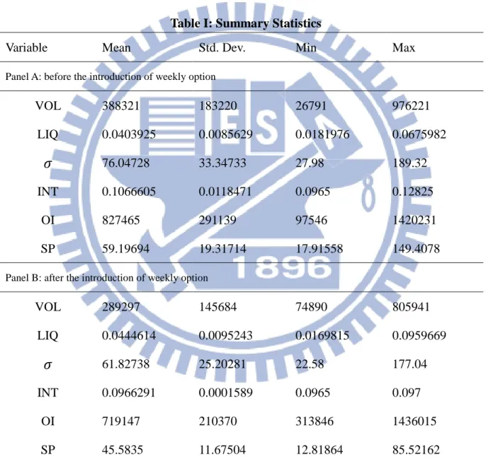
Summary statistics of primary variables are illustrated below in Table I with 518 observations of each variable, which are the trading days between Jan 2011 and Dec 2013 in the TXO market. The data are divided into two parts by the introduction date of weekly option. It briefly explains the mean and standard deviation of variables. Firstly, before the introduction of weekly option, the mean of trade volume, proportional bid-ask spread, and open interests are 388321, 0.0403925, and 827465 respectively, while the values are 289297, 0.0444614, and 719147, respectively, after the introduction. There exists a significant change in the mean of volume and open interest. Although the mean of the spreads have only a little change, but the maximum of proportional bid-ask spread is .0675982 before the introduction and 0.0959669 after. The mean of traded volume and open interest of monthly options decreased, but the mean of spreads increased. The mean of price volatility of the underlying market is 76.04728, with a maximum of 189.32 before weekly option listing, while the mean

0 100000 200000 300000 400000 500000 600000 0 250000 500000 750000 1000000 1250000

Monthly Volume Weekly Volume

(21)

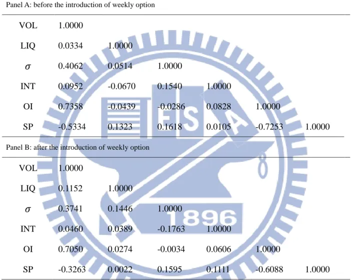
is 61.82738 with a maximum of 177.04 after that. Interest rates have an average of 0.1066605 before the introduction, with an average of 0.0966291 after, and are not volatile. Table II is the correlation table of variables used in the simultaneous equations.The data are also divided into two parts by the introduction of weekly option. Directions in panel A and B are mostly the same except that the relationship between bid-ask spread and open interest, interest rate, and the relationship between price volatility and interest rate are different.

Table I: Summary Statistics

Variable Mean Std. Dev. Min Max

Panel A: before the introduction of weekly option

VOL 388321 183220 26791 976221 LIQ 0.0403925 0.0085629 0.0181976 0.0675982

𝜎𝜎

76.04728 33.34733 27.98 189.32 INT 0.1066605 0.0118471 0.0965 0.12825 OI 827465 291139 97546 1420231 SP 59.19694 19.31714 17.91558 149.4078

Panel B: after the introduction of weekly option

VOL 289297 145684 74890 805941 LIQ 0.0444614 0.0095243 0.0169815 0.0959669

𝜎𝜎

61.82738 25.20281 22.58 177.04 INT 0.0966291 0.0001589 0.0965 0.097 OI 719147 210370 313846 1436015 SP 45.5835 11.67504 12.81864 85.52162

This table reports the summary statistics of the dataset before and after weekly option listing. Trade volume, denoted by VOL, is the daily total trade volume of the two nearest month index options in one day. LIQ is the

proportional bid-ask spread calculated as 𝐿𝐿𝐿𝐿𝐿𝐿_𝑡𝑡 =

∑𝑎𝑎𝑖𝑖=1𝑉𝑉𝑉𝑉𝐿𝐿𝑖𝑖_{�𝑎𝑎𝑎𝑎𝑎𝑎 𝑖𝑖+𝑏𝑏𝑖𝑖𝑏𝑏 𝑖𝑖�/2}𝑎𝑎𝑎𝑎𝑎𝑎 𝑖𝑖−𝑏𝑏𝑖𝑖𝑏𝑏 𝑖𝑖

∑𝑎𝑎𝑖𝑖=1𝑉𝑉𝑉𝑉𝐿𝐿𝑖𝑖 . 𝜎𝜎is the price volatilityof the underlying market, which is the gap between the highest traded price and the lowest traded price of the underlying asset in

(22)

one day. INT is the Interbank Overnight Call-Loan Rate. The scale of interest rate is adjusted to 100 times larger than the original value. OI is the total open interest of the two nearest month index options in one day.SP is the daily weighted average settlement price with volumes to be weights.

Table II: Correlations between independent variables

Variable VOL LIQ

𝜎𝜎

INT OI SP

Panel A: before the introduction of weekly option

VOL 1.0000 LIQ 0.0334 1.0000

𝜎𝜎

0.4062 0.0514 1.0000 INT 0.0952 -0.0670 0.1540 1.0000 OI 0.7358 -0.0439 -0.0286 0.0828 1.0000 SP -0.5334 0.1323 0.1618 0.0105 -0.7253 1.0000

Panel B: after the introduction of weekly option

VOL 1.0000 LIQ 0.1152 1.0000

𝜎𝜎

0.3741 0.1446 1.0000 INT 0.0460 0.0389 -0.1763 1.0000 OI 0.7050 0.0274 -0.0034 0.0606 1.0000 SP -0.3263 0.0022 0.1595 0.1111 -0.6088 1.0000

This table reports the correlations between independent variables before and after weekly option listing. VOL is

the daily trade volume. LIQ is the proportional bid-ask spread. 𝜎𝜎is the price volatilityof the underlying market.

INT is the Interbank Overnight Call-Loan Rate. OI is the daily open interest. SP is the daily weighted average settlement price.

(23)

4.2 The impacts on volume, spread, and price volatility

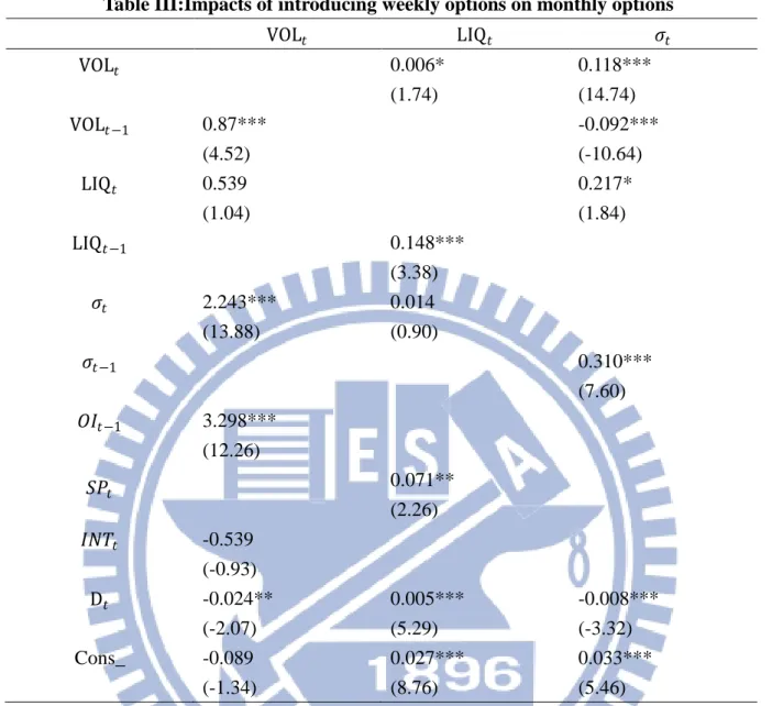
The regression results of the first simultaneous equations model are displayed in Table III. First of all, thecoefficients of dummy variables are -0.024, 0.005, and -0.008 for volume, liquidity, and price volatility respectively at a significance level of 1%, which indicatesthat introducing weekly option decreases the trading volume, increases the spreads of monthly options, and reduces the price volatility of the underlying market. Secondly, the spreads of monthly option significantly increased, which means that the liquidity of monthly option decreased. Thirdly, the price volatility significantly decreased, indicating that weekly option listing stabilizes the underlying market. The results are consistent with the first three hypotheses: (1)the introduction of weekly options would take over the volume of monthly options causing a decrease in volume of monthly option; (2)there would be a decrease in the liquidity of monthly options because of the decrease in the volume; (3)price volatility of the underlying security would decrease.Most research focus on the impacts on the whole option market, while this study focus on the original TXO monthly options.Theresults are consistent with the view that introducing related new derivatives such as mini-futures and short maturity options would supplant its original security’s volume. However, prior studies have also shown that the volume of the whole option market still rises after the introduction of weekly option. On the other hand, these new financial instruments might lessen information asymmetry, resulting in lower price volatility in the underlying market (Shenbagaraman (2003), Liu (2007)). Besides dummy variable, lagging variables are all statistically significant, which means not only weekly options but also the information of the prior period of monthly option itself affect the spread and volatility of monthly options. In detail, besides lagging trading volumes negatively affect volatility, other lagging variables are all positively correlated with spreads.

(24)

Table III:Impacts of introducing weekly options on monthly options VOL𝑡𝑡 LIQ𝑡𝑡 𝜎𝜎𝑡𝑡 VOL𝑡𝑡 0.006* (1.74) 0.118*** (14.74) VOL𝑡𝑡−1 0.87*** (4.52) -0.092*** (-10.64) LIQ𝑡𝑡 0.539 (1.04) 0.217* (1.84) LIQ𝑡𝑡−1 0.148*** (3.38) 𝜎𝜎𝑡𝑡 2.243*** (13.88) 0.014 (0.90) 𝜎𝜎𝑡𝑡−1 0.310*** (7.60) 𝑉𝑉𝐿𝐿𝑡𝑡−1 3.298*** (12.26) 𝑆𝑆𝑆𝑆𝑡𝑡 0.071** (2.26) 𝐿𝐿𝐼𝐼𝐼𝐼𝑡𝑡 -0.539 (-0.93) D𝑡𝑡 -0.024** (-2.07) 0.005*** (5.29) -0.008*** (-3.32) Cons_ -0.089 (-1.34) 0.027*** (8.76) 0.033*** (5.46)

The simultaneous equations are: 𝑉𝑉𝑉𝑉𝐿𝐿_𝑡𝑡 = 𝑎𝑎₀+ 𝑎𝑎₁𝐿𝐿𝐿𝐿𝐿𝐿_𝑡𝑡+ 𝑎𝑎₂𝜎𝜎_𝑡𝑡+ 𝑎𝑎₃𝐿𝐿𝐼𝐼𝐼𝐼_𝑡𝑡+ 𝑎𝑎₄𝑉𝑉𝐿𝐿_𝑡𝑡−1+ 𝑎𝑎₅𝑉𝑉𝑉𝑉𝐿𝐿_𝑡𝑡−1+ 𝑎𝑎₆𝐷𝐷_𝑡𝑡+ 𝜀𝜀_1𝑡𝑡,

𝐿𝐿𝐿𝐿𝐿𝐿𝑡𝑡 = 𝑏𝑏0+ 𝑏𝑏1𝑉𝑉𝑉𝑉𝐿𝐿𝑡𝑡+ 𝑏𝑏2𝜎𝜎𝑡𝑡+ 𝑏𝑏3𝑆𝑆𝑆𝑆𝑡𝑡+ 𝑏𝑏4𝐿𝐿𝐿𝐿𝐿𝐿𝑡𝑡−1+ 𝑏𝑏5𝐷𝐷𝑡𝑡+ 𝜀𝜀2𝑡𝑡,and 𝜎𝜎𝑡𝑡 = 𝑐𝑐0+ 𝑐𝑐1𝑉𝑉𝑉𝑉𝐿𝐿𝑡𝑡+ 𝑐𝑐2𝐿𝐿𝐿𝐿𝐿𝐿𝑡𝑡+ 𝑐𝑐3𝑉𝑉𝑉𝑉𝐿𝐿𝑡𝑡−1+

𝑐𝑐4𝜎𝜎𝑡𝑡−1+ 𝑐𝑐5𝐷𝐷𝑡𝑡+ 𝜀𝜀3𝑡𝑡.VOL is the daily trade volume. LIQ is the proportional bid-ask spread. 𝜎𝜎is the price

volatilityof the underlying market. INT is the Interbank Overnight Call-Loan Rate. OI is the daily open interest. SP is the daily weighted average settlement price. Coefficient scales are adjusted so that coefficient scales would

be alike. VOL, OI, 𝜎𝜎, SP are 1/1,000,000, 1/10,000,000, 1/1,000, and 1/1,000 of its original value respectively.

This adjustment is also used in regressions afterwards. Significance level: ***:1%, **:5%, *:10%

4.3 The impacts near settlement days and the expiration day effect

To take into account the influence of maturity, we mainly focus on the last week of settlement, which are the last trading days before settlement days. Using simultaneous

equation approach with an additional dummy variable,𝐷𝐷₂, allows us to analyze the impacts of

(25)

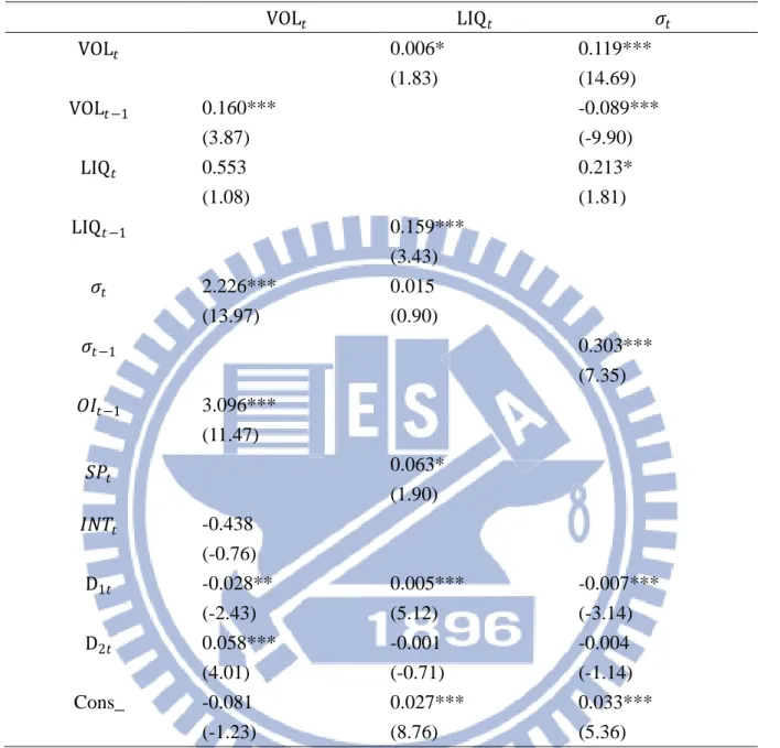
weekly options in weeks of settlement before and after the introduction of weekly options. Results are displayed in Table IV below. Most of the primary independent variables have only tiny changes on their coefficients except for the trade volume of monthly options. The directions of variables in Table II, especially dummy variable, remain unchanged, which

means the impacts generally remain the same in settlement week.The coefficient of 𝐷𝐷₁on

volume decreased from -0.024 to -0.028 at 5% significancelevel, indicating that weekly options affects monthly options more in this period. Impacts on liquidity and price volatility are almost identical as in normal days. Nevertheless, the opposite directions on coefficients of

𝐷𝐷1 and 𝐷𝐷2 make it hard to determine the impacts of weekly option listing on monthly options

near settlement, which is consistent with our last hypothesis.

The expiration day effect

In the settlement week before expiration day, trade volume of monthly options

significantly increases due to the expiration day effect. Thecoefficient of 𝐷𝐷₂ on volume hasa

positive number of 0.058 at 1% significance level. This is consistent with most of the empirical results of expiration day effects, causing abnormal volume during settlement periods (Stoll and Whaley (1987), Hseu (2008), Chou et al. (2012)).However, coefficients of liquidity and price volatility appear to be not significant with small coefficient values, indicating that there are no obvious expiration day effects in liquidity and price volatility in this period. This is might because the impacts of expiration day effects in liquidity and price volatility are overlapped by impacts of introducing weekly options, therefore causing the

insignificance of coefficients on 𝐷𝐷₂. The results here show that although weekly options were

introduced, the expiration day effects still exist on trading volume, which implies that there may still exists some information asymmetry in the market. The results are the same after considering moneynessin Table V.

(26)

Table IV:Impacts of introducing weekly options on monthly options near expiration daysand the expiration day effect

VOL𝑡𝑡 LIQ𝑡𝑡 𝜎𝜎𝑡𝑡 VOL𝑡𝑡 0.006* (1.83) 0.119*** (14.69) VOL𝑡𝑡−1 0.160*** (3.87) -0.089*** (-9.90) LIQ𝑡𝑡 0.553 (1.08) 0.213* (1.81) LIQ𝑡𝑡−1 0.159*** (3.43) 𝜎𝜎𝑡𝑡 2.226*** (13.97) 0.015 (0.90) 𝜎𝜎𝑡𝑡−1 0.303*** (7.35) 𝑉𝑉𝐿𝐿𝑡𝑡−1 3.096*** (11.47) 𝑆𝑆𝑆𝑆𝑡𝑡 0.063* (1.90) 𝐿𝐿𝐼𝐼𝐼𝐼𝑡𝑡 -0.438 (-0.76) D1𝑡𝑡 -0.028** (-2.43) 0.005*** (5.12) -0.007*** (-3.14) D2𝑡𝑡 0.058*** (4.01) -0.001 (-0.71) -0.004 (-1.14) Cons_ -0.081 (-1.23) 0.027*** (8.76) 0.033*** (5.36)

In this table, we include another dummy variable,𝐷𝐷₂, to further examine the impacts in the last week to

settlement. The simultaneous equations are:𝑉𝑉𝑉𝑉𝐿𝐿_𝑡𝑡 = 𝑎𝑎₀+ 𝑎𝑎₁𝐿𝐿𝐿𝐿𝐿𝐿_𝑡𝑡+ 𝑎𝑎₂𝜎𝜎_𝑡𝑡+ 𝑎𝑎₃𝐿𝐿𝐼𝐼𝐼𝐼_𝑡𝑡+ 𝑎𝑎₄𝑉𝑉𝐿𝐿_𝑡𝑡−1+ 𝑎𝑎₅𝑉𝑉𝑉𝑉𝐿𝐿_𝑡𝑡−1+

𝑎𝑎6𝐷𝐷1𝑡𝑡+ 𝑎𝑎7𝐷𝐷2𝑡𝑡+ 𝜀𝜀1𝑡𝑡, 𝐿𝐿𝐿𝐿𝐿𝐿𝑡𝑡 = 𝑏𝑏0+ 𝑏𝑏1𝑉𝑉𝑉𝑉𝐿𝐿𝑡𝑡+ 𝑏𝑏2𝜎𝜎𝑡𝑡+ 𝑏𝑏3𝑆𝑆𝑆𝑆𝑡𝑡+ 𝑏𝑏4𝐿𝐿𝐿𝐿𝐿𝐿𝑡𝑡−1+ 𝑏𝑏5𝐷𝐷1𝑡𝑡+ 𝑏𝑏6𝐷𝐷2𝑡𝑡+ 𝜀𝜀2𝑡𝑡, and 𝜎𝜎𝑡𝑡 = 𝑐𝑐0+ 𝑐𝑐1𝑉𝑉𝑉𝑉𝐿𝐿𝑡𝑡+ 𝑐𝑐2𝐿𝐿𝐿𝐿𝐿𝐿𝑡𝑡+ 𝑐𝑐3𝑉𝑉𝑉𝑉𝐿𝐿𝑡𝑡−1+ 𝑐𝑐4𝜎𝜎𝑡𝑡−1+ 𝑐𝑐5𝐷𝐷1𝑡𝑡+ 𝑐𝑐6𝐷𝐷2𝑡𝑡+ 𝜀𝜀3𝑡𝑡.𝐷𝐷2represents whether the transactions occur in

this period (equals 1 for being in the period), while 𝐷𝐷₁ still represents the introduction of weekly options.VOL is

the daily trade volume. LIQ is the proportional bid-ask spread. 𝜎𝜎is the price volatilityof the underlying market.

INT is the Interbank Overnight Call-Loan Rate. OI is the daily open interest. SP is the daily weighted average settlement price. Significance levels: ***:1%, **:5%, *:10%

(27)

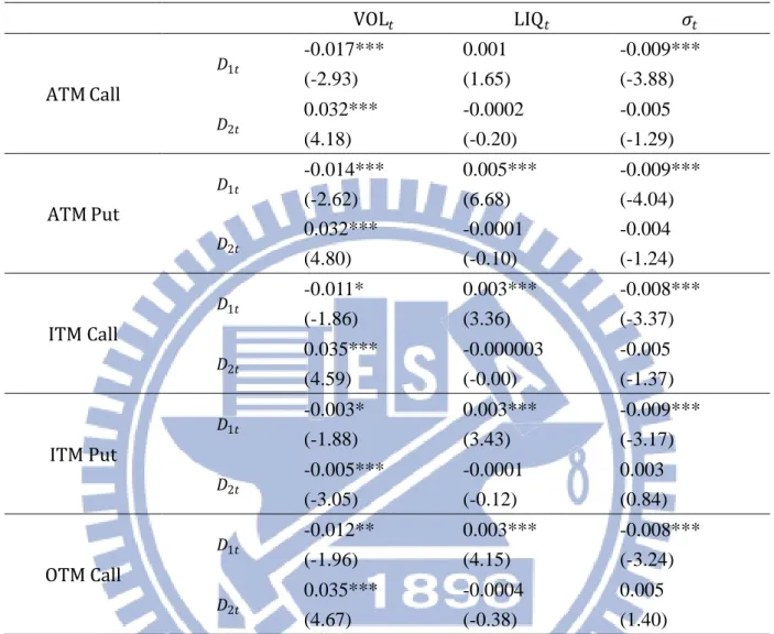
4.4 The impacts considering moneyness and types of options Table V: Coefficients of dummy variables of Model (2)

VOL𝑡𝑡 LIQ𝑡𝑡 𝜎𝜎𝑡𝑡 ATM Call 𝐷𝐷1𝑡𝑡 -0.017*** (-2.93) 0.001 (1.65) -0.009*** (-3.88) 𝐷𝐷2𝑡𝑡 0.032*** (4.18) -0.0002 (-0.20) -0.005 (-1.29) ATM Put 𝐷𝐷1𝑡𝑡 -0.014*** (-2.62) 0.005*** (6.68) -0.009*** (-4.04) 𝐷𝐷2𝑡𝑡 0.032*** (4.80) -0.0001 (-0.10) -0.004 (-1.24) ITM Call 𝐷𝐷1𝑡𝑡 -0.011* (-1.86) 0.003*** (3.36) -0.008*** (-3.37) 𝐷𝐷2𝑡𝑡 0.035*** (4.59) -0.000003 (-0.00) -0.005 (-1.37) ITM Put 𝐷𝐷1𝑡𝑡 -0.003* (-1.88) 0.003*** (3.43) -0.009*** (-3.17) 𝐷𝐷2𝑡𝑡 -0.005*** (-3.05) -0.0001 (-0.12) 0.003 (0.84) OTM Call 𝐷𝐷1𝑡𝑡 -0.012** (-1.96) 0.003*** (4.15) -0.008*** (-3.24) 𝐷𝐷2𝑡𝑡 0.035*** (4.67) -0.0004 (-0.38) 0.005 (1.40)

In this table, coefficients of dummy variables are reported. Dataset are divided into three categories by moneyness. ATM, ITM, and OTM are abbreviations of at-the-money, in-the-money, and out-of-the-money respectively. The range of moneyness is determined using K/S ratio. K/S ratio of ATM options ranges from 0.93 to 1.07. The regression of OTM put options has insufficient observations so that results are absent. VOL is the

daily trade volume. LIQ is the proportional bid-ask spread. 𝜎𝜎is the price volatilityof the underlying market.

Significance levels: ***:1%, **:5%, *:10%

In this section, the dataset are divided into six categories by moneyness and types of options. The range of moneyness is the same as mentioned above. Results are displayed below from Table VI to Table XV and also reorganized by taking out coefficients of dummy variables, which is Table V below. The impacts of introducing weekly option, which are the

(28)

coefficients of D_1𝑡𝑡, appear to be different among moneyness. First of all, impacts are similar in the same moneyness category regardless of call or put. Coefficients’ directions of the three variables are also identical in all option categories. However, impacts are not apparent only on spreads of ATM call options. Looking at the impacts of weekly option listing and taking into account of moneyness, three variables have different results. As of volume, decreases are more apparent on ATM options than the others. In general, time value has a maximum on ATM options, which favors sellers who want to earn profits from time value decrease. The property of weekly options allow sellers to have another choice to short options with shorter duration and therefore the market uncertaintyof longer duration would be lessen. As a result, volume transfers from monthly options to weekly options. In contrast, spreads increase more apparently in all kinds of options except for ATM call options. This is probably also a result after volume decreased because the liquidity of monthly options decreases after lower volume and appears larger spreads. Price volatility is the only variable that decreases are similar in all kinds of options, both directions and values. This is probably because price volatility is a market property, not a property of individual or specific security. So the influence has no difference among moneyness.

Secondly, as time goes near settlement, the coefficients of D_2𝑡𝑡tell the influence of time

to maturity on monthly options. Results still appear to have expiration day effect on volume of monthly options, while liquidity and price volatility seems to be not affected by time to

maturity. Besides, the significance and values of coefficients of D_1𝑡𝑡 are all similar to model

(1). This indicates two important messages:(1)impacts of weekly option listing do not change regardless of time to maturity; (2)expiration day effects still significantly appear in monthly options after weekly optionlisting. For detailed results, tables are displayed in the appendix.

Alike the impacts of most index options on its underlying securities, the introduction of weekly option also decreased the volume of monthly options. Moreover, liquidity also decreased, which is differentfrom other studies. For example, Chen and Chung (2011) showed

(29)

that the introduction of SPDR options improves the liquidity of SPDRs.This is probably because our research objective is monthly options, not the whole TXO market. Prior research focus on the whole market including the new derivative. Price volatility of the underlying market decreased after weekly option listing, which supports the view of prior research, such as Damodaran and Lim (1991), and Liu (2007) both reach the same conclusion that stock index options can stabilize its underlying market.Shenbagaraman (2003) also suggests that futures and options listing do not destabilize the underlying market but also improves liquidity in India market. However, some studies still show that new futures/option listing may not stabilize the underlying market. Ma and Rao (1988) found that volatilestocks become more stable after option listing, while stable stocks become more volatile after option listing. The most obvious and opposite example is the research by Trede and Wahrenburg (1997) who found that German stock returns became more volatileafter introduction of options at the DeutscheTerminbörse (DTB). Therefore, it is still not sure whether option listing stabilizes the underlying market or not.

(30)

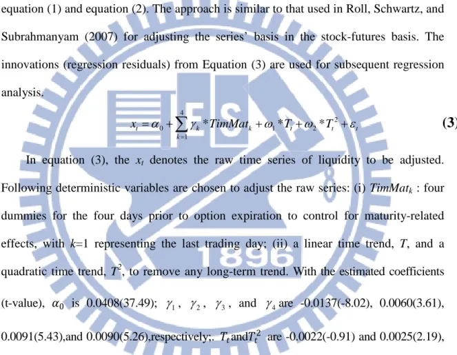
5 Robustness Analysis

Previous studies report that raw series data with time trend and common regularities may result in spurious conclusions in the regression analyses. To solve the potential spuriousness problem, we adjust the time-series of liquidity for deterministic variables using regression equation (3) before proceeding with the simultaneous equation in equation (1) and equation (2). The approach is similar to that used in Roll, Schwartz, and Subrahmanyam (2007) for adjusting the series’ basis in the stock-futures basis. The innovations (regression residuals) from Equation (3) are used for subsequent regression analysis. 4 2 0 1 2 1 * * * t k k t t t k x α γ TimMat ω T ω T ε = = +

∑

+ + +

(3)

In equation (3), the xt denotes the raw time series of liquidity to be adjusted.

Following deterministic variables are chosen to adjust the raw series: (i) TimMatk : four

dummies for the four days prior to option expiration to control for maturity-related effects, with k=1 representing the last trading day; (ii) a linear time trend, T, and a

quadratic time trend, T2, to remove any long-term trend. With the estimated coefficients

(t-value), 𝛼𝛼₀ is 0.0408(37.49); γ₁, γ₂, γ₃, and γ₄are -0.0137(-8.02), 0.0060(3.61),

0.0091(5.43),and 0.0090(5.26),respectively;. 𝐼𝐼_𝑡𝑡and𝐼𝐼_𝑡𝑡2 are -0.0022(-0.91) and 0.0025(2.19),

respectively. The regression R-square is 0.2398 (>0), suggesting that the chosen variable explain a non-trivial portion of liquidity.

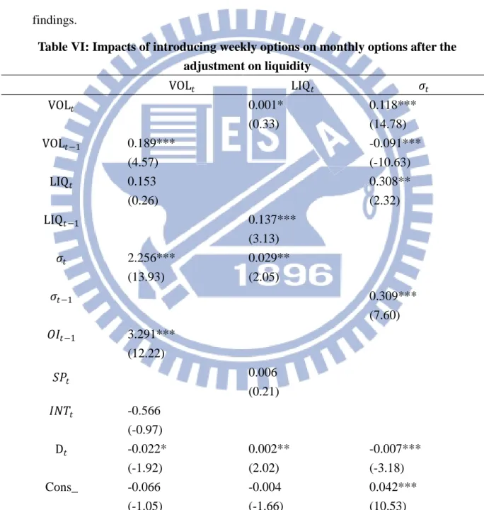
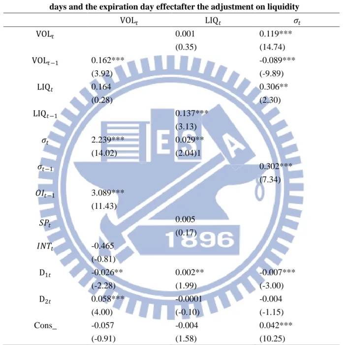
Table VII and Table VIII reportthe regression results after the adjustment on liquidity.Results reveal that, no matter trading activities happened on the settlement week or not, the impacts of weekly option listing on trade volume and liquidity of monthly options, and price volatility of underlying index remain the same with those in section 4.

In Table VII, the coefficients of 𝐷𝐷_𝑡𝑡on fortrade volume, liquidity, and price volatility are

(31)

-0.022, 0.002, and -0.007 at significance level of 10%, 5%, and 1%,

respectively.However, in Table VIII, the coefficients of 𝐷𝐷_1𝑡𝑡for VOL_𝑡𝑡, LIQ_𝑡𝑡, and

𝜎𝜎𝑡𝑡become -0.026, 0.002, and -0.007 at significance level of 5%, 5%, and 1% respectively.

The coefficients of D_2𝑡𝑡 for VOL_𝑡𝑡, LIQ_𝑡𝑡, and 𝜎𝜎_𝑡𝑡 are 0.058 , -0.0001 and -0.004 with

only 0.058at 1% significance level, which are also identical with results before adjustment. Results of regressions based on optionmoneyness are similar with the prior findings.

Table VI: Impacts of introducing weekly options on monthly options after the adjustment on liquidity VOL𝑡𝑡 LIQ𝑡𝑡 𝜎𝜎𝑡𝑡 VOL𝑡𝑡 0.001* (0.33) 0.118*** (14.78) VOL𝑡𝑡−1 0.189*** (4.57) -0.091*** (-10.63) LIQ𝑡𝑡 0.153 (0.26) 0.308** (2.32) LIQ𝑡𝑡−1 0.137*** (3.13) 𝜎𝜎𝑡𝑡 2.256*** (13.93) 0.029** (2.05) 𝜎𝜎𝑡𝑡−1 0.309*** (7.60) 𝑉𝑉𝐿𝐿𝑡𝑡−1 3.291*** (12.22) 𝑆𝑆𝑆𝑆𝑡𝑡 0.006 (0.21) 𝐿𝐿𝐼𝐼𝐼𝐼𝑡𝑡 -0.566 (-0.97) D𝑡𝑡 -0.022* (-1.92) 0.002** (2.02) -0.007*** (-3.18) Cons_ -0.066 (-1.05) -0.004 (-1.66) 0.042*** (10.53)

VOL is the daily trade volume. LIQ is the proportional bid-ask spread. However, factors that might affect liquidity, such as time-to-maturity and temporal trends, are taken off from the raw time-series data through the

(32)

equation 4 2 0 1 2 1 * * * t k k t t t k x α γ TimMat ω T ω T ε =

= +

∑

+ + + .𝜎𝜎is the price volatility of the underlying market. INT is the Interbank Overnight Call-Loan Rate. OI is the daily open interest. SP is the daily weighted average settlement price. Significance levels: ***:1%, **:5%, *:10%

Table VII:Impacts of introducing weekly options on monthly options near expiration days and the expiration day effectafter the adjustment on liquidity

VOL𝑡𝑡 LIQ𝑡𝑡 𝜎𝜎𝑡𝑡 VOL𝑡𝑡 0.001 (0.35) 0.119*** (14.74) VOL𝑡𝑡−1 0.162*** (3.92) -0.089*** (-9.89) LIQ𝑡𝑡 0.164 (0.28) 0.306** (2.30) LIQ𝑡𝑡−1 0.137*** (3.13) 𝜎𝜎𝑡𝑡 2.239*** (14.02) 0.029** (2.04)1 𝜎𝜎𝑡𝑡−1 0.302*** (7.34) 𝑉𝑉𝐿𝐿𝑡𝑡−1 3.089*** (11.43) 𝑆𝑆𝑆𝑆𝑡𝑡 0.005 (0.17) 𝐿𝐿𝐼𝐼𝐼𝐼𝑡𝑡 -0.465 (-0.81) D1𝑡𝑡 -0.026** (-2.28) 0.002** (1.99) -0.007*** (-3.00) D2𝑡𝑡 0.058*** (4.00) -0.0001 (-0.10) -0.004 (-1.15) Cons_ -0.057 (-0.91) -0.004 (1.58) 0.042*** (10.25)

VOL is the daily trade volume. LIQ is the proportional bid-ask spread. However,factors that might affect liquidity, such as time-to-maturity and temporal trends, are taken off from the raw time-series data through the equation

4 2 0 1 2 1 * * * t k k t t t k x α γ TimMat ω T ω T ε =

= +

∑

+ + + .𝜎𝜎 is the price volatilityof the underlying market. INT is the Interbank Overnight Call-Loan Rate. OI is the daily open interest. SP is the daily weighted average settlement

price. 𝐷𝐷₂represents whether the transactions occur in this period (equals 1 for being in the period), while 𝐷𝐷₁

still represents the introduction of weekly options. Significance levels: ***:1%, **:5%, *:10%

(33)

6 Conclusion

This paper provides empirical results of the impacts of weekly options on thevolume, liquidity of monthly options and the price volatility of its underlying market by applying a simultaneous equation approach. Firstly, we find that launching weekly options significantly decreases the volume and liquidity of monthly options.Secondly, the introduction also stabilizes the underlying market by decreasing its price volatility. In the second part, we use another dummy variable and focus on the last week of settlement to see whether the impacts on volume, liquidity of monthly options and the price volatility of its underlying market become more apparent or not. Results show that impacts of weekly option listing generally remain unchanged during settlement week. Only trade volume significantly increases due to expiration day effects. These results are consistent with our hypotheses.

In the third part, the results based on moneyness and types of options,show that weekly option listing influence trade volumeeven more in at-the-money options, while impactson liquidity are more apparent in in-the-money and out-of-the-money options.

In addition, we also obtain the same results after adjusting the raw data of liquidity by removingthe effect of time-to-maturity and time trend.Even controlling for moneyness and option types, the impacts of weekly option listing also remain identical as those results before the adjustments..

(34)

7 Reference

[1] Bansal, V. K., Pruitt, S. W., & Wei, K. C., An empirical reexamination of the impact of CBOE option initiation on the volatility and trading volume of the underlying equities: 1973–1986, Financial Review, 24(1), 19-29, 1989.

[2] Bessembinder, H., & Seguin, P. J., Price volatility, trading volume, and marketdepth: Evidence from futures markets, Journal of financial and QuantitativeAnalysis, 28(01), 21-39, 1993.

[3] Bollen, Nicolas P.B., A note on the impact of options on stock return volatility, Journal ofBanking and Finance v22: 1181-1191, 1998.

[4] Cao, M., & Wei, J., Option market liquidity: Commonality and othercharacteristics, Journal of Financial Markets, 13(1), 20-48, 2010.

[5] Chatrath, A., Kamath, R., Chakornpipat, R., &Ramchander, S., Lead-lag associations between option trading and cash market volatility. Applied Financial Economics, 5(6), 373-381, 1995.

[6] Chen, D. H., & Chang, P. H., The impact of listing stock options on the underlying securities: the case of Taiwan. Applied Financial Economics, 18(14), 1161-1172, 2008.

[7] Chen, W. P., & Chung, H., Has the introduction of S&P 500 ETF options led to improvements in price discovery of SPDRs?, Journal of Futures Markets, 32(7), 683-711, 2012.

[8] Chernov, M., &Ghysels, E., A study towards a unified approach to the joint estimation of objective and risk neutral measures for the purpose of options valuation, Journal offinancial economics, 56(3), 407-458, 2000.

[9] Chordia, T., Roll, R., &Subrahmanyam, A., Commonality in liquidity. Journal of Financial Economics, 56(1), 3-28, 2000.

(35)

[10] Chordia, T., Roll, R., &Subrahmanyam, A., Market liquidity and trading activity. The Journal of Finance, 56(2), 501-530, 2001.

[11] Chow, Y. F., Yung, H. H., & Zhang, H., Expiration day effects: The case of Hong Kong, Journal of Futures Markets, 23(1), 67-86, 2003.

[12] Chow, E. H. Y., Hung, C. W., Liu, C. S. H., &Shiu, C. Y., Expiration day effects and market manipulation: evidence from Taiwan, Review of Quantitative Finance and Accounting, 41(3), 441-462, 2013.

[13] Chung, H., &Hseu, M. M., Expiration day effects of Taiwan index futures: The case of the Singapore and Taiwan Futures Exchanges, Journal of International Financial Markets, Institutions and Money, 18(2), 107-120, 2008.

[14] Damodaran, A., & Lim, J., The effects of option listing on the underlying stocks' return processes, Journal of Banking & Finance, 15(3), 647-664, 1991.

[15] Freund, Steven, P. Douglas McCann and Gwendolyn P. Webb, A Regression Analysis of the Effects of option introduction on stock variances, Journal of Derivatives v1: 25-38, 1994.

[16] Hasan, M. K., & Chowdhury, S. The impact of the Introduction of index options on volatility and liquidity on the underlying stocks.

[17] Heer, B., Trede, M., &Wahrenburg, M., The effect of option trading at the DTB on the underlying stocks' return variance. Empirical Economics, 22(2), 233-245, 1997. [18] Jegadeesh, N., &Subrahmanyam, A., Liquidity effects of the introduction of the S&P

500 index futures contract on the underlying stocks. Journal of Business, 171-187, 1993

[19] Kumar, R., Sarin, A., &Shastri, K., The impact of index options on the underlying stocks: The evidence from the listing of Nikkei stock average options, Pacific-Basin Finance Journal, 3(2), 303-317, 1995.

(36)

[20] Kumar, R., Sarin, A., &Shastri, K., The impact of options trading on the marketquality of the underlying security: An empirical analysis,The Journal of Finance, 53(2), 717-732, 1998.

[21] Lamoureux, Christopher G. and Sunil K. Panikkath, 1994, Variations in Stock Returns: Asymmetriesand other patterns, working paper.

[22] Liu, S., The impacts of index options on the underlying stocks: The case of the S&P 100, The Quarterly Review of Economics and Finance, 49(3), 1034-1046, 2009.

[23] Mayhew, S., &Mihov, V., Another look at option listing effects, Institute forQuantitative Research in Finance, 2000.

[24] Pilar, C., & Rafael, S., Does derivatives trading destabilize the underlying assets?

Evidence from the Spanish stock market, Applied Economics Letters, 9(2),107-110, 2002.

[25] Roll, R., Schwartz, E., and Subrahmanyam, A., Liquidity and the Law of One Price: The Case of the Futures–Cash Basis. Journal of Finance, 62, 2201-2234, 2007

[26] Shenbagaraman, P., Do futures and options trading increase stock market volatility? NSE News Letter, NSE Research Initiative, Paper, (20), 2003.

[27] Skinner, D. J., Options markets and stock return volatility, Journal of Financial Economics, 23(1), 61-78, 1989.

[28] Wang, Y., Chung, H., & Yang, Y., The market fragmentation impact of E-mini futures on the liquidity of open-outcry index futures,International Research Journalof Finance and Economics, 12, 165-180, 2007.

[29] Wei, P., Poon, P. E. R. C. Y., & Zee, S., The effect of option listing on bid-ask spreads, price volatility, and trading activity of the underlying OTC stocks, Review of

Quantitative Finance and Accounting, 9(2), 165-180, 1997.

[30] Xu, C., Expiration‐Day Effects of Stock and Index Futures and Options in Sweden: The Return of the Witches, Journal of futures markets, 2013.

(37)

8 Appendix

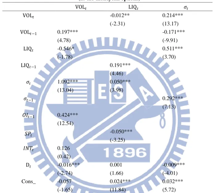
Table VIII: Impacts of introducing weekly options on monthly options (at-the-moneycall options) VOL𝑡𝑡 LIQ𝑡𝑡 𝜎𝜎𝑡𝑡 VOL𝑡𝑡 -0.012** (-2.31) 0.214*** (13.17) VOL𝑡𝑡−1 0.197*** (4.78) -0.171*** (-9.91) LIQ𝑡𝑡 -0.546* (-1.78) 0.511*** (3.70) LIQ𝑡𝑡−1 0.191*** (4.46) 𝜎𝜎𝑡𝑡 1.092*** (13.04) 0.050*** (3.98) 𝜎𝜎𝑡𝑡−1 0.292*** (7.13) 𝑉𝑉𝐿𝐿𝑡𝑡−1 0.424*** (12.54) 𝑆𝑆𝑆𝑆𝑡𝑡 -0.050*** (-3.25) 𝐿𝐿𝐼𝐼𝐼𝐼𝑡𝑡 0.126 (0.42) D𝑡𝑡 -0.016*** (-2.74) 0.001 (1.66) -0.009*** (-4.01) Cons_ -0.057 (-1.65) 0.024*** (11.84) 0.032*** (5.72)

VOL is the daily trade volume. LIQ is the proportional bid-ask spread. 𝜎𝜎is the price volatility of the underlying

market. INT is the Interbank Overnight Call-Loan Rate. OI is the daily open interest. SP is the daily weighted average settlement price.Significance levels: ***:1%, **:5%, *:10%

(38)

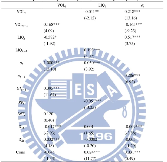
Table IX:Impacts of introducing weekly options on monthly options near expiration days and the expiration day effect(at-the-money call options)

VOL𝑡𝑡 LIQ𝑡𝑡 𝜎𝜎𝑡𝑡 VOL𝑡𝑡 -0.011** (-2.12) 0.218*** (13.16) VOL𝑡𝑡−1 0.168*** (4.09) -0.165*** (-9.23) LIQ𝑡𝑡 -0.582* (-1.92) 0.517*** (3.75) LIQ𝑡𝑡−1 0.193*** (4.37) 𝜎𝜎𝑡𝑡 1.080*** (13.10) 0.050*** (3.92) 𝜎𝜎𝑡𝑡−1 0.286*** (6.92) 𝑉𝑉𝐿𝐿𝑡𝑡−1 0.395*** (11.64) 𝑆𝑆𝑆𝑆𝑡𝑡 -0.051*** (-3.25) 𝐿𝐿𝐼𝐼𝐼𝐼𝑡𝑡 0.120 (0.40) D1𝑡𝑡 -0.017*** (-2.93) 0.001 (1.65) -0.009*** (-3.88) D2𝑡𝑡 0.032*** (4.18) -0.0002 (-0.20) -0.005 (-1.29) Cons_ -0.045 (-1.33) 0.024*** (11.77) 0.031*** (5.49)

(39)

Table X: Impacts of introducing weekly options on monthly options (at-the-money put options)

VOL𝑡𝑡 LIQ𝑡𝑡 𝜎𝜎𝑡𝑡 VOL𝑡𝑡 0.029*** (4.93) 0.256*** (14.07) VOL𝑡𝑡−1 0.268*** (6.33) -0.208*** (-10.73) LIQ𝑡𝑡 0.059 (0.21) 0.402*** (2.94) LIQ𝑡𝑡−1 0.146*** (3.46) 𝜎𝜎𝑡𝑡 0.952*** (12.70) -0.006 (6.78) 𝜎𝜎𝑡𝑡−1 0.296*** (7.29) 𝑉𝑉𝐿𝐿𝑡𝑡−1 0.365*** (10.61) 𝑆𝑆𝑆𝑆𝑡𝑡 0.087*** (6.78) 𝐿𝐿𝐼𝐼𝐼𝐼𝑡𝑡 -0.202 (-0.76) D𝑡𝑡 -0.013** (-2.47) 0.005*** (6.69) -0.009*** (-4.12) Cons_ -0.025 (-0.82) 0.013*** (7.68) 0.035*** (6.68)

(40)

Table XI:Impacts of introducing weekly options on monthly options near expiration days and the expiration day effect(at-the-money put options)

VOL𝑡𝑡 LIQ𝑡𝑡 𝜎𝜎𝑡𝑡 VOL𝑡𝑡 0.030*** (4.70) 0.260*** (14.05) VOL𝑡𝑡−1 0.226*** (5.34) -0.201*** (-9.96) LIQ𝑡𝑡 0.046 (0.17) 0.402*** (2.95) LIQ𝑡𝑡−1 0.147*** (3.40) 𝜎𝜎𝑡𝑡 0.945*** (12.87) -0.006 (-0.48) 𝜎𝜎𝑡𝑡−1 0.288*** (7.03) 𝑉𝑉𝐿𝐿𝑡𝑡−1 0.341*** (10.04) 𝑆𝑆𝑆𝑆𝑡𝑡 0.086*** (6.75) 𝐿𝐿𝐼𝐼𝐼𝐼𝑡𝑡 -0.174 (-0.67) D1𝑡𝑡 -0.014*** (-2.62) 0.005*** (6.68) -0.009*** (-4.04) D2𝑡𝑡 0.032*** (4.80) -0.0001 (-0.10) -0.004 (-1.24) Cons_ -0.020 (-0.66) 0.013*** (7.60) 0.034*** (6.56)

(41)

Table XII: Impacts of introducing weekly options on monthly options (in-the-money call options)

VOL𝑡𝑡 LIQ𝑡𝑡 𝜎𝜎𝑡𝑡 VOL𝑡𝑡 -0.001 (-0.25) 0.220*** (13.56) VOL𝑡𝑡−1 0.248*** (6.02) -0.169*** (-9.72) LIQ𝑡𝑡 -0.508 (-1.61) 0.465*** (3.39) LIQ𝑡𝑡−1 0.198*** (4.60) 𝜎𝜎𝑡𝑡 0.1.079*** (12.59) 0.038*** (3.06) 𝜎𝜎𝑡𝑡−1 0.291*** (7.08) 𝑉𝑉𝐿𝐿𝑡𝑡−1 0.285*** (10.41) 𝑆𝑆𝑆𝑆𝑡𝑡 0.00001 (0.37) 𝐿𝐿𝐼𝐼𝐼𝐼𝑡𝑡 -0.521* (-1.70) D𝑡𝑡 -0.008 (-1.38) 0.003*** (3.37) -0.008*** (-3.57) Cons_ 0.018 (0.55) 0.020*** (12.35) 0.031*** (5.67)

(42)

Table XIII:Impacts of introducing weekly options on monthly options near expiration days and the expiration day effect(in-the-money call options)

VOL𝑡𝑡 LIQ𝑡𝑡 𝜎𝜎𝑡𝑡 VOL𝑡𝑡 -0.011 (-0.23) 0.224*** (13.57) VOL𝑡𝑡−1 0.211*** (5.12) -0.162*** (-8.98) LIQ𝑡𝑡 -0.532* (-1.72) 0.470*** (3.43) LIQ𝑡𝑡−1 0.199*** (4.46) 𝜎𝜎𝑡𝑡 1.071*** (12.75) 0.038*** (3.01) 𝜎𝜎𝑡𝑡−1 0.283*** (6.83) 𝑉𝑉𝐿𝐿𝑡𝑡−1 0.264*** (9.67) 𝑆𝑆𝑆𝑆𝑡𝑡 0.00001 (0.37) 𝐿𝐿𝐼𝐼𝐼𝐼𝑡𝑡 -0.485 (-1.61) D1𝑡𝑡 -0.011* (-1.86) 0.003*** (3.36) -0.008*** (-3.37) D2𝑡𝑡 0.035*** (4.59) -0.000003 (-0.00) -0.005 (-1.37) Cons_ 0.027 (0.79) 0.020*** (12.01) 0.030*** (5.43)

(43)

Table XIV: Impacts of introducing weekly options on monthly options (in-the-money put options)

VOL𝑡𝑡 LIQ𝑡𝑡 𝜎𝜎𝑡𝑡 VOL𝑡𝑡 -0.030 (-1.66) 0.760*** (9.30) VOL𝑡𝑡−1 0.584*** (16.52) -0.592*** (-7.02) LIQ𝑡𝑡 -0.078 (-1.01) 0.544*** (3.66) LIQ𝑡𝑡−1 0.178*** (4.14) 𝜎𝜎𝑡𝑡 0.169*** (8.13) 0.037*** (3.07) 𝜎𝜎𝑡𝑡−1 0.202*** (4.81) 𝑉𝑉𝐿𝐿𝑡𝑡−1 0.025*** (2.78) 𝑆𝑆𝑆𝑆𝑡𝑡 0.110*** (2.83) 𝐿𝐿𝐼𝐼𝐼𝐼𝑡𝑡 0.252*** (3.23) D𝑡𝑡 -0.003* (-1.81) 0.003*** (3.46) -0.009*** (-3.24) Cons_ -0.028*** (-3.32) 0.019*** (12.06) 0.040*** (6.92)

(44)

Table XV:Impacts of introducing weekly options on monthly options near expiration days and the expiration day effect(in-the-money put options)

VOL𝑡𝑡 LIQ𝑡𝑡 𝜎𝜎𝑡𝑡 VOL𝑡𝑡 -0.030 (-1.66) 0.766*** (9.33) VOL𝑡𝑡−1 0.565*** (15.84) -0.592*** (-7.01) LIQ𝑡𝑡 -0.061 (-0.80) 0.539*** (3.63) LIQ𝑡𝑡−1 0.180*** (4.04) 𝜎𝜎𝑡𝑡 0.169*** (8.22) 0.037*** (3.07) 𝜎𝜎𝑡𝑡−1 0.202*** (4.81) 𝑉𝑉𝐿𝐿𝑡𝑡−1 0.033*** (3.50) 𝑆𝑆𝑆𝑆𝑡𝑡 0.011*** (2.81) 𝐿𝐿𝐼𝐼𝐼𝐼𝑡𝑡 0.258*** (3.33) D1𝑡𝑡 -0.003* (-1.88) 0.003*** (3.43) -0.009*** (-3.17) D2𝑡𝑡 -0.005*** (-3.05) -0.0001 (-0.12) 0.003 (0.84) Cons_ -0.029*** (-3.46) 0.019*** (12.03) 0.040*** (6.80)

週選擇權上市對台灣選擇權市場流動性之衝擊探討

國立交通大學

資訊管理與財務金融學系

財務金融碩士班

碩 士 論 文

週選擇權上市對台灣選擇權市場流動性之衝擊探討

Impacts of Introducing Weekly Options on the Liquidity of

Option Market in Taiwan

研究生：周承儀

指導教授：鍾惠民教授

周幼珍教授

Impacts of Introducing Weekly Options on the Liquidity of

Option Market in Taiwan

研究生：周承儀

Student：Cheng-Yi Chou

指導教授：鍾惠民、周幼珍 Advisor：Huimin Chung

Yow-Jen Jou

國 立 交 通 大 學

資訊管理與財務金融學系

財務金融碩士班

碩 士 論 文 初 稿

中 華 民 國 一 百 零 三 年 七 月

週選擇權上市對台灣選擇權市場流動性之衝擊探討

國立交通大學 資訊管理與財務金融學系 財務金融碩士班

中 文 摘 要

Impacts of Introducing Weekly Options on the Liquidity of

Option Market in Taiwan

Graduate Program of Finance

Department of Information Management and Finance

National Chiao Tung University

Abstract

Acknowledgments

Table of Contents

Figures and Tables

1 Introduction

2 Literature Review

3 Data & Methodology

𝑳𝑳𝑳𝑳𝑳𝑳

=

∑

𝑽𝑽𝑽𝑽𝑳𝑳

∑

𝑽𝑽𝑽𝑽𝑳𝑳

4 Empirical Results

𝜎𝜎

𝜎𝜎

𝜎𝜎

𝜎𝜎

𝜎𝜎

5 Robustness Analysis

∑

(3)

∑

∑

6 Conclusion

7 Reference

8 Appendix

碩士論文

國立交通大學

碩士論文初稿

中華民國一百零三年七月

國立交通大學資訊管理與財務金融學系財務金融碩士班

中文摘要