使用開放式精簡指令集處理器應用於即時偵測失神性癲癇動物模型之軟硬體共同實現

(1)

國立交通大學

電信工程研究所

碩士論文

使用開放式精簡指令集處理器

應用於即時偵測失神性癲癇動物模型之軟硬體共同實現

Software-hardware Co-implementation for Real-time Epileptic

Seizure Detection Using OpenRISC Processor Core on

Absence Animal Models

研究生：張舜婷

指導教授：闕河鳴

(2)

(3)

使用開放式精簡指令集處理器

應用於即時偵測失神性癲癇動物模型之軟硬體共同實現

Software-hardware Co-implementation for Real-time Epileptic

Seizure Detection Using OpenRISC Processor Core on Absence

Animal Models

研究生：張舜婷 Student: Shun-Ting Chang 指導教授：闕河鳴 Advisor: Herming Chiueh

國立交通大學

電信工程研究所

碩士論文

A Thesis

Submitted to Institute of Communications Engineering College of Electrical and Computer Science

National Chiao Tung University in Partial Fulfillment of the Requirements

for the Degree of Master of Science in Communication Engineering December 2011 Hsinchu, Taiwan 中華民國一百年十二月

(4)

使用開放式精簡指令集處理器

應用於即時偵測失神性癲癇動物模型之軟硬體共同實現

研究生：張舜婷指導教授：闕河鳴國立交通大學電信工程研究所碩士論文

摘要

癲癇是一種最常見的神經系統失調疾病之一，全球有 1%的人罹患癲癇，25%的癲癇病患無法完全被治癒。在過去幾年，開迴路的癲癇控制器已經被提出，如迷走神經刺激和腦深部刺激，但連續性或間歇性的電刺激會導致高功率消耗以及神經細胞損害的可能性。相反的，近年來閉迴路的硬體和生理訊號處理器已經被提出。但這些研究中，在癲癇發作 5 秒後才會偵測到癲癇或者是沒有提及偵測時間。此外，大部分的研究通常是利用片段的腦電圖驗證癲癇演算法，無法全然地證實演算法的健全性。因此，在過去我們提出一套無線可攜式即時癲癇偵測與抑制系統，並使用連續性的腦電圖長時間偵測癲癇。在本篇論文中，改進上述所提出的即時癲癇偵測閉迴路系統的決定參數方式，提出一個快速決定參數方法，使這些參數最適合每個老鼠的模型。這個快速決定參數方法比先前決定參數的方法快了 416106 倍，同時也可達到 92-99%的高偵測率以及可以在 0.63-0.79 秒偵測到癲癇。此外，使用精簡指令集的技術實現一個低功耗的生理訊號處理器，將偵測癲癇演算法實現在生理訊號處理器上可達到即時處理生理訊號以及只消耗 6 mW。與先前提出的系統比較，可以降低 93.8%的功率消耗。本篇所提出的癲癇偵測器可應用於即時偵測系統中，以及在未來可以與類比前端電路和後端刺激器整合成一個積體化的閉迴路偵測系統。

(5)

Software-hardware Co-implementation for Real-time Epileptic

Seizure Detection Using OpenRISC Processor Core on Absence

Animal Models

Student: Shun-Ting Chang Advisor: Herming Chiueh SoC Design Lab, Institute of Communications Engineering,

College of Electrical and Computer Science, National Chiao Tung University, Hsinchu 30010, Taiwan

Abstract

Epilepsy is one of the most common neurological disorders. Approximately 1% of people in the world suffer from epilepsy, and 25% of epilepsy patients cannot be healed by today’s available treatments. In past years, open-loop seizure controllers have been proposed, such us vagus nerve stimulation and deep brain stimulation devices; however, the device drives a stimulator continuously or intermittently that causes high power consumption and the likelihood of neuronal damage. In contrast, the closed-loop implementation of hardware prototypes or biomedical signal processors has been proposed recently. Nevertheless, the average of seizure detection delay is either longer than 5 seconds or often not mentioned in these works, and it is insufficient to validate the robustness of detection algorithm. Moreover, most of studies often use the discontinuous electroencephalogram (EEG) signal fragments to validate seizure detection algorithm. As a result, a portable wireless online closed-loop seizure controller in freely moving rats was proposed, which validated seizure detection algorithm by using continuous online EEG signals.

(6)

In this thesis, the fast parameter determination method, which determines a fitting model for each rat, is proposed to improve our previous work. The proposed parameter determination method is 416106 times faster than our previous work, and it can attain the same detection accuracy (92-99%) and detection delay (0.63-0.79 s). Additionally, a low-power biomedical signal processor which bases on reduced instruction set computer (RISC) technology consumes only 6 mW for real-time epileptic seizure detection algorithm. Compared with our previous prototype, the measurement results show that the implemented processor can reduce 93.8% power consumption. The developed seizure detector can be applied to monitor the online EEG signals and integrate with analog front-end circuitries and an electrical stimulator to perform a closed-loop seizure controller in the future.

(7)

Acknowledgements

經過了兩年半，終於實現了生日願望。這兩年半，曾經很茫然，不知道要做什麼，要休學要放棄的念頭出現過好幾百回，最後還是膽小地不敢放棄。到如今可以拿到碩士學位，首先，我要感謝我的老師闕河鳴，您讓我學習到思考要有邏輯，做事情要有效率以及口語表達的能力，讓我在可以進入社會前，可以有一個紮實的訓練。緊接著，我要感謝燦杰學長，不管在我修課以及研究中給予我不少幫助，感謝學長時常抽空跟我討論問題以及指點我研究的方式。還有筱筑學姐常常幫助我們解決行政的流程和常常載我們出去玩。再來，我要感謝剛進實驗室時，學長們的經驗傳承，讓我可以提早適應研究生活。以及，我要感謝我的同學鄭錡，常常一起奮戰到半夜，半夜鬼吼鬼叫，同甘共苦，同進同退，雖已同年同月同日生、同年同月同日同高中畢業，一定也要同年同月同日同研究所畢業。以及我另一個同學文仲常常跟我討論研究上的問題，分享生活上的芝麻小事。還有實驗室學弟妹們餅乾、俐嵐、俊達、嘉倫和蔡頭，常常一起跟腦袋不靈光的學姐腦力激盪，還有口試時的鼎力相助，真是讓我太感動了。還要謝謝研究所的同學們維盈無論是學術上和生活上，都給予我極大的幫助。以及修 ICLAB 認識的恰克，有著一同寫作業的革命情感，總是有聊不完的話，說不完的天。還要謝謝在南部的丸子，三天兩頭聽我打電話哭訴，總是告訴我這樣就放棄也太弱了，聽完這句話就會超不服氣地反駁他，我才不是那樣的人。最後要感謝我的家人，告訴我進來交大就是來學習的，不是來混一張紙畢業的，不會就要學，不懂就要問，讓我能繼續堅持下去，謝謝他們。舜婷

(8)

List of Tables

Table 5.1 Summary of the proposed low-power BSP. ... 36

Table 6.1 Observed SWD duration and two selected frequency bands. ... 47

Table 6.2 Accuracy and false detection of the epileptic seizure detection algorithm. ... 48

Table 6.3 Performance of two parameter determination methods. ... 48

(11)

List of Figures

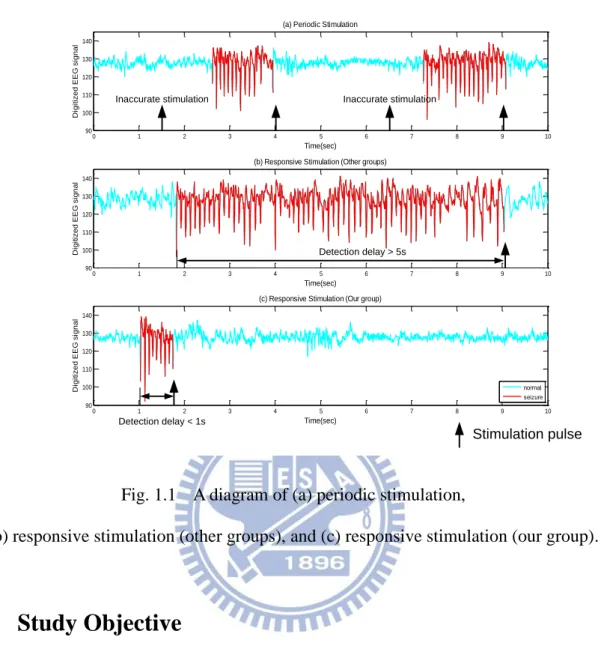
Fig. 1.1 A diagram of (a) periodic stimulation, (b) responsive stimulation (other groups),

and (c) responsive stimulation (our group). ... 3

Fig. 2.1 EEG examples during the wakefulness (WK), spike-wave discharge (SWD), slow-wave sleep (SWS), and movement artifact. ... 7

Fig. 3.1 Closed-loop epileptic seizure control system ... 8

Fig. 3.2 Closed-loop epileptic seizure control system based on enhanced 8051 microcontroller. ... 10

Fig. 4.1 Overall procedure in closed-loop seizure detection system. ... 12

Fig. 4.2 Window size and window shift are applied to feature extraction. ... 13

Fig. 4.3 Data size of EEG signals for CM calculation. ... 16

Fig. 4.4 Computation of the S1 value. ... 16

Fig. 4.5 Computation of the S2 value. ... 17

Fig. 4.6 Complexity measurement in four behavioral states... 17

Fig. 4.7 Spectral analysis in four behavioral states. ... 18

Fig. 4.8 Using correlations analysis identifies spectral indexes (Band1 and Band2). ... 19

Fig. 4.9 Result of correlation analysis. ... 21

Fig. 4.10 Data size of EEG signals for FFT calculation. ... 21

Fig. 4.11 64-point radix-4 FFT decimation-in-time algorithm. ... 23

Fig. 4.12 An example of LLS classifier’s input X. ... 26

Fig. 4.13 Procedure of training phase. ... 27

Fig. 4.14 Feature extraction and LLS classifier training... 28

Fig. 4.15 The flowchart of seizure determination. ... 28

(12)

Fig. 4.17 Flowchart of fast parameter determination method. ... 31

Fig. 4.18 (a) Original data, (b) Determine T1, (c) Determine THSWS, (d) Determine T2 and TLSWS. ... 32

Fig. 4.19 Procedure of testing phase. ... 33

Fig. 4.20 Flowchart of on-line seizure detection algorithm. ... 33

Fig. 5.1 (a) Block diagram of OR1200 processor, (b) Block diagram of the proposed low-power BSP. ... 35

Fig. 5.2 The (a) chip layout and (b) die photo of the implemented low-power BSP. ... 36

Fig. 5.3 Flowchart of (a) data acquisition, (b) seizure detection, and (c) stimulation pulse generation. ... 37

Fig. 5.4 (a) The proposed timing diagram, (b) Original timing diagram. ... 38

Fig. 5.5 Original data flow. ... 39

Fig. 5.6 The proposed data flow. ... 40

Fig. 6.1 Functional block diagram of experiment setup. ... 43

Fig. 6.2 The testing board of the proposed low-power BSP with FPGA-based evaluation platform... 43

Fig. 6.3 Function verification flow... 44

Fig. 6.4 Timing diagram of the seizure detection firmware. ... 45

Fig. 6.5 EEG data and the seizure events detection by proposed BSP. (a) SWD in WK state, (b) SWD in SWS state, (c) false detection in SWS state. ... 46

Fig. 6.6 EEG containing multiple absence seizure SWDs and detected seizure events by proposed low-power BSP. ... 48

(13)

Chapter 1 Introduction

Epilepsy is one of the most common neurological disorders. Approximately 1% of people in the world suffer from epilepsy, and 25% of epilepsy patients cannot be healed by today’s available treatments [1, 2]. If seizures cannot be well controlled, the patients experience major limitations in family, social, educational, and vocational activities.

1.1 Motivation

Recently, numerous alternative techniques have been proposed, such us vagus nerve and deep brain stimulation devices [1, 2]. Most of the devices utilize open-loop controller to suppress the seizure. However, an open-loop controller drives a stimulator continuously or intermittently that causes high power consumption and the likelihood of neuronal damage. In contract, a closed-loop device combines a stimulator and seizure detector. Recently, one closed-loop epilepsy control system developed by NeuroPace called Responsive Neurostimulator (RNS®) System is in U.S. FDA clinical trials [2]. A closed-loop device can increase stimulus efficacy and reduce tissue damage over the long term. A closed-loop seizure controller drives a stimulator when a closed-loop device detects the seizure [2-4]. Despite additional hardware, a closed-loop device can increase stimulus efficacy and reduce tissue damage over the long term. As a result, compared with open-loop devices, closed-loop devices is more effective and attractive. In general, a robust on-line seizure detection method, which can drive antiepileptic device to suppress the seizure as early as possible when a seizure happens, is required for the development of a closed-loop seizure controller.

(14)

Recently, the implementation of hardware prototypes and biomedical signal processors has been proposed [5-19]. Among these projects, wavelet analysis, spectral analysis, entropy analysis, and variance analysis are applied to detect seizure events. Some closed-loop seizure controllers utilized analog to extract seizure features so epileptic seizure detection accuracy was high [15, 18]. Some seizure detection algorithm relied on powerful processing platform keeping real-time seizure detection and high detection accuracy [9-11, 13, 17]. However, the average response time for seizure detection is either longer than 5 seconds or often not mentioned in these works. Moreover, most of studies often use the discontinuous electroencephalogram (EEG) signal fragments to validate seizure detection algorithm; nevertheless, it is deficient in validating the robustness of detection algorithm. As a result, a portable wireless online closed-loop seizure controller in freely moving rats was proposed [20-23], which validated seizure detection algorithm by using continuous online EEG signals. Furthermore, the detection delay is shorter than 1 second. To summarize, an open-loop seizure controller with periodic stimulation is inaccurate and inefficient as shown in Fig. 1.1 (a). A closed-loop seizure controller with responsive stimulation which is proposed by other groups as mentioned above is more accurate and efficient; however, the detection delay is longer than 5 seconds as shown in Fig. 1.1 (b). Fig. 1.1 (c) shows that a closed-loop seizure controller with responsive stimulation is proposed by our group. When a seizure occurs, the responsive stimulator starts to suppress the seizure, and the detection delay is shorter than 1 second.

(15)

0 1 2 3 4 5 6 7 8 9 10 90 100 110 120 130 140

(a) Periodic Stimulation

D ig it ize d E E G si g n a l Time(sec) 0 1 2 3 4 5 6 7 8 9 10 90 100 110 120 130 140

(b) Responsive Stimulation (Other groups)

D ig it ize d E E G si g n a l Time(sec) 0 1 2 3 4 5 6 7 8 9 10 90 100 110 120 130 140

(c) Responsive Stimulation (Our group)

D ig it ize d E E G si g n a l Time(sec) normal seizure Detection delay < 1s Inaccurate stimulation Detection delay > 5s Inaccurate stimulation Stimulation pulse

Fig. 1.1 A diagram of (a) periodic stimulation,

(b) responsive stimulation (other groups), and (c) responsive stimulation (our group).

1.2 Study Objective

In our previous work, using implied approximate entropy and 64-point fast Fourier transform, which contained large portion of digital processing, increased detection rate. In order to decrease complex calculation and hardware area, a liner least squares (LLS) was classifier in this project. Furthermore, it was observed that most of false detections occurred in slow-wave sleep (SWS) state, so adaptive thresholds were utilized to switch the threshold of the LLS for decreasing false detection rate. However, adaptive thresholds were obtained by using exhaustive key search in training phase; as a result, this method wasted a lot of time on training phase. In addition, implementation based on 8051-like microcontroller [24] consumed more than 117mW to perform the real-time seizure detection.

(16)

In this study, it is proposed that using the mean and standard deviation of EEG training data searches adaptive thresholds rapidly. The new parameter determination method is faster than our previous work, and it can attain same performance. Moreover, the seizure detection algorithm in previous work is implemented in a RISC-like processor to suppress seizures. The flexibility, simplicity, and fixed instruction format of RISC [25] is feasible implementation with high processing performance. Although more complicate hardware architecture is used to realize real-time seizure detection, the RISC-like processor does not run algorithm at full speed in processing biomedical signals. As a result, a slower clock rate is applied to reduce the power and energy consumption of the proposed system. The continuous EEG signals of four Long-Evens rats are applied to the proposed biomedical signal processor. The results show the embedded processor is robustly processing 24 hours long-term and uninterrupted EEG sequence. In the future, the development of proposed processor will integrate analog front-end and antiepileptic circuitries into system-on-a-chip design for neural prosthesis applications.

1.3 Thesis Organization

The content of this thesis is organized as follows. Chapter 1 introduces the motivation and objective of this work. Chapter 2 describes the preparation of animal models and recorded EEG training data. In Chapter 3, the system architecture of proposed biomedical signal processor is described. Chapter 4 presents the epileptic seizure detection algorithm and the proposed parameter determination method. Chapter 5 demonstrates the hardware and firmware implementation. In Chapter 6, the evaluation procedure and measurement results are presented. Finally the conclusion and future work are made in Chapter 7.

(17)

Chapter 2 EEG Data Acquisition

In this thesis, we use EEG signals of absence animal models to validate our seizure detection algorithm. As a result, first, we introduce what absence seizure is, how we prepare general animals, and how we define four state of continuous EEG recording.

2.1 Absence Seizure

Absence seizures are one of several kinds of seizures. These seizures are sometimes referred to as petit mal seizures. People may appear to be staring into space blankly. These periods last for seconds, or even tens of seconds. Sometimes, those experiencing absence seizures move from one location to another without any purpose. In normal circumstances thalamo-cortical oscillations maintain normal consciousness of an individual. However, in abnormal circumstances the normal pattern may be disrupted; as a result, people are led to an episode of absence [26].

The spike-wave discharge (SWD) is the archetype electroencephalographic characteristic of non-convulsive epilepsy. SWDs can be found in various types of absence epilepsy, including childhood absence epilepsy, juvenile absence epilepsy, juvenile myoclonic epilepsy, myoclonic absence epilepsy, eyelid myoclonia with absence epilepsy, and generalized tonic-clonic seizures in some patients.

Nowadays, genetic rodent models, such as GAERS and WAG/Rij rats, are most commonly used for studying new antiepileptic drugs, basic mechanisms of seizures and seizure related neurophysiological and neurochemical activities and processes. The frequency of the discharges in genetic rodent strains is 7-10 Hz [27, 28].

(18)

2.2 General Animal Preparation

Adult Long-Evans rats with spontaneous spike-and-wave discharge (SWD) are used in the thesis. There are two seizure types of Long-Evans rats in previous work, including absence seizures and pentylenetetrazol (PTZ) induced seizures. The genetic defect of Long-Evans rats causes spontaneous SWD. The EEG characteristic of spontaneous SWD is much closer to epileptic patients’ EEG than PTZ induced SWD in the clinical aspect.

In this thesis, Long-Evans rats were 4-6 months old, and their weight was 500-700 grams. The rats were placed in a room under a 12:12-hour light-dark cycle with food and water provided ad libitum. All surgical and experimental procedures were reviewed and approved by the Institutional Animal Care and Use Committee of the National Cheng Kung University. The rats were anesthetized with sodium pentobarbital (50 mg/kg, i.p.). Subsequently, it was placed in a standard stereotaxic apparatus. Screw electrodes were bilaterally implanted over the area of the frontal barrel cortex (anterior 2.0 mm, lateral 2.0 mm with regard to the bregma). A four-microwire bundle, which was made of Teflon-insulated stainless steel microwires (#7079, A-M Systems), was used to stimulate the right-side zona incerta (ZI) (posterior 4.0 mm, lateral 2.5 mm, and depth 6.7-7.2 mm). A ground electrode was implanted 2 mm caudal to the lambda. Dental cement was applied to fasten the connection socket to the surface of the skull. Following suturing to complete the surgery, animals were given antibiotics and housed individually in cages for recovery.

Two weeks after the surgery, each animal was placed in the recording environment at least two times (1 hour/day) prior to testing to allow rats to habituate to the experimental apparatus. In this procedure, about 90% of Long-Evans rats showed spontaneous SWD, which were used for continuous EEG recording. Continuous EEG recording from 5 hours to 24 hours (contained one circadian cycle) were recorded and analyzed to assess our seizure detector in this thesis.

(19)

2.3 Continuous EEG Recording

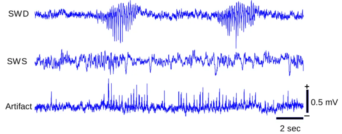
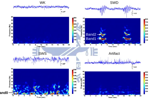
In order to validate the robust of seizure detection algorithm, EEG recording must be continuous and uninterrupted for monitoring and analyzing. Fig. 2.1 shows an example of EEG recording corresponding to various behavioral states, including wakefulness (WK), spike-wave discharge (SWD), slow-wave sleep (SWS), and movement artifact in continuous recording of Long-Evans rats.

In this thesis, two essential processing phases of EEG data were performed in Long-Evans, including a training phase and a testing phase. In the training phase, continuous EEG data of each rat were recorded for feature extraction without enabling electrical stimulation. Then, marking recorded EEG data corresponds to seizures (SWD) and non-seizures (WK, SWS, and artifact) by specialist. After four states (SWD, WK, SWS, and artifact) of EEG data were used to train the seizure program off-line, the parameters of a seizure detection model were determined. In the testing phase, after applying the especial parameters to each rat, we proceeding to on-line closed-loop seizure detection. The details of training and testing methods describe in Chapter 4.

Fig. 2.1 EEG examples during the wakefulness (WK), spike-wave discharge (SWD), slow-wave sleep (SWS), and movement artifact.

+ _ 0.5 mV + _ + _ + _ + _ + _ 2 sec W K SWD SWS Artifact

(20)

Chapter 3 System Architecture

This chapter describes system architecture of closed-loop epileptic seizure control system. The detail of epileptic seizure controller is also introduced. In previous work, a seizure controller has been implemented based on an enhanced 8051 microcontroller. In this thesis, in order to achieve high performance, the seizure controller is implemented by OpenRISC processor.

3.1 Closed-Loop Epileptic Seizure Control System

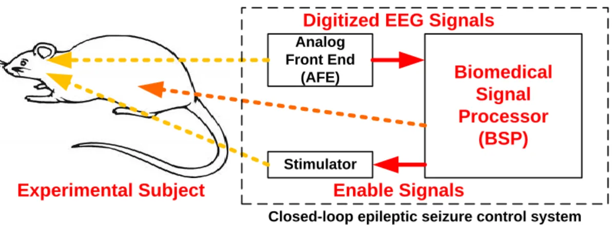
The closed-loop epileptic seizure control system is composed of three modules: 1) an analog front end (AFE); 2) a biomedical signal processor; and 3) a stimulator. The functional block diagram of the closed-loop epileptic seizure control system is illustrated in Fig. 3.1. The AFE transforms EEG signals into digitized EEG signals. The BSP processes digitized EEG signals. When the BSP detects seizures, it generates enable signals to stimulator. Then, the stimulator generates electric current to suppress seizures.

Biomedical Signal Processor (BSP) Analog Front End (AFE) Stimulator

Experimental Subject Enable Signals Digitized EEG Signals

Closed-loop epileptic seizure control system

(21)

In this thesis, the seizure detection scheme is based on a large proportion of digital signal processing. Much technology have the high capability of processing digital signals, such as field-programmable gate array (FPGA), DSP, application-specific integrated circuit (ASIC), and RISC processor. Modern high-density FPGA can incorporate embedded processor with custom hardware accelerator to attain high performance; nonetheless, it consumes high static power (tens of milliwatts to hundreds of milliwatts) because of its advanced fabrication technology. ASIC is an integrated circuit, which is highly specialized for particular scenarios or applications. This solution is highly optimized in terms of area, power, and speed to perform its designated task, but it is lack of flexibility. DSP also has high processing capability, but it consumes power consumption highly because of other dedicated hardware accelerators which are not required in our algorithm. Hence, a general purpose processor is chosen in this research.

3.2 General Purpose Processor

3.2.1 Enhanced 8051 Microcontroller

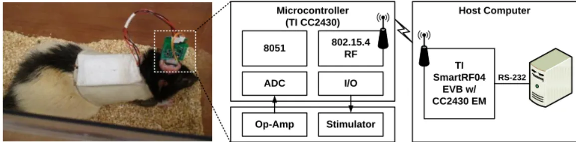
In our previous work [20-23], a seizure controller has been implemented based on an enhanced 8051 microcontroller in freely moving rats. The seizure controller was comprised of a signal conditioning circuit, a microcontroller, and a stimulator. As shown in Fig. 3.2, a closed-loop seizure controller was carried by an experimental subject, and a host computer monitored spontaneous brain activities, which were communicated based on a wireless ZigBee protocol. The EEG signals were amplified and band-pass filtered by the signal conditioning block. Based on a single-channel, 200-Hz sampling rate, and 10-bit ADC resolution, the microcontroller and the signal conditioning circuit consumed 117.66 mW. The power consumption of biomedical implementation is significant for implantable devices.

(22)

Microcontroller (TI CC2430) 802.15.4 RF ADC I/O Op-Amp Stimulator 8051 TI SmartRF04 EVB w/ CC2430 EM Host Computer RS-232

Fig. 3.2 Closed-loop epileptic seizure control system based on enhanced 8051 microcontroller.

3.2.2 OpenRISC Processor

Modern 32-bit RISC processors deliver better energy efficiency than traditional 8-bit microcontrollers. Therefore, a powerful 32-bit processor which is OpenRISC 1200 (OR1200) [29] is modified and implemented for real-time and low-power epileptic seizure detection. In addition, it provides over one dhrystone 2.1 MIPS (DMIPS) per MHz and one DSP MAC 3232 operations per MHz, and the speed of OpenRISC 1200 is up to 10 times faster than an enhanced 8051 microprocessor’s (about 0.1 DMIPS/MHz [30], [31]). In biomedical application, energy efficiency is an important characteristic of biomedical implant, so how low power and energy is the central concern in this work. Our experimental results show the energy per seizure event determination is about 1.15 mJ for OpenRISC and 18.8 mJ for enhanced 8051 microprocessor. The details of evaluation results are described in Chapter 6. The characteristic of OpenRISC is energy efficiency and flexibility; as a result, it can be applied to not only epileptic seizure detection but also other biomedical applications.

(23)

Chapter 4 Epileptic Seizure Detection Algorithm

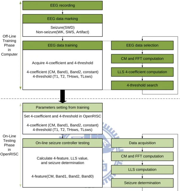
This chapter describes the overall procedure and the seizure detection algorithm [32, 33] in our closed-loop epileptic seizure control system. Briefly speaking, two essential stages of EEG signal processing are performed in Long-Evans rats in this thesis as illustrated in Fig. 4.1. The overall procedure consists of the off-line training phase and the on-line testing phase.

In training phase, continuous EEG signals of each rat are recorded for marking and training. After recorded, EEG signals which correspond to seizures (SWD) and non-seizures (WK, SWS, and artifact) are marked by specialist. The marked events as mentioned above are used to extract complexity measurement (CM) and fast Fourier transform (FFT) values, train linear least square (LLS) classifier and search the finest thresholds (T1 for WK, T2 for SWS, TLSWS, and THSWS) in our closed-loop seizure control system.

In testing phase, while the parameters of a seizure detection model, which include 4-coefficient of LLS classifier and 4-threshold of seizure determination, are determined, the parameters are downloaded to our processor. Finally, on-line seizure detection testing is performed in OpenRISC.

The following are the details of feature extraction and classifier. Moreover, the details of proposed training flow and testing flow are also described in 4.3.

(24)

EEG recording

EEG data marking

EEG data training

Parameters setting from training

On-line seizure controller testing Seizure(SWD) Non-seizure(WK, SWS, Artifact)

Acquire 4-coefficient and 4-threshold

4-coefficient (CM, Band1, Band2, constant) 4-threshold (T1, T2, THsws, TLsws)

Set 4-coefficient and 4-threshold in OpenRISC

4-coefficient (CM, Band1, Band2, constant) 4-threshold (T1, T2, THsws, TLsws) Off-Line Training Phase in Computer On-Line Testing Phase in OpenRISC LLS 4-coefficient computation 4-threshold search LLS computation Seizure determination Calculate 4-feature, LLS value,

and seizure determination

4-feature(CM, Band1, Band2, Band0)

EEG data selection

CM and FFT computation

Data acquisition

(25)

4.1 Feature Extraction

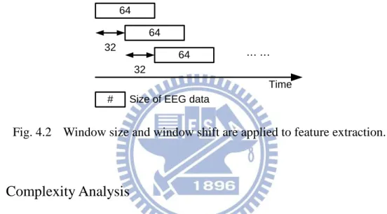
Fig. 4.2 shows that 64 points of EEG data are packed with 32 points overlap from previous 64 points of EEG data. In this thesis, combining chaotic and frequency domain analysis can attain high detection accuracy and low computational cost. Complexity analysis such as entropy can distinguish between WK and SWD [34]. The frequency bands of power changes correlate closely with SWD. Spectral analysis can perform as the complementary features of entropy to reduce false detection during SWS or movement artifact.

# Size of EEG data 64 64 64 32 32 Time … …

Fig. 4.2 Window size and window shift are applied to feature extraction.

4.1.1 Complexity Analysis

The EEG signals of a seizure are more ordered than those in normal state; as a result, entropy has been used to analyze and detect the seizure. In order to reduce computational cost, simplified entropy which is approximate entropy (ApEn) has been proposed for real-time processing [34]. The value of the ApEn is determined as shown in the following.

1) Give an N-point time-series of data, which is formed the same space in time. X is represented to be

   

1 , 2 , ,

 

X _x x  x N _ ( 1 )

2) Let x(i) be a subsequence of X; that is,

 

i _x i

  

,x i1 ,



,x i



 m 1 , for 1



_    i N m 1

x ( 2 )

(26)

3) Define d[x(i), x(j)], which is the maximum difference of the relative elements in vectors x(i) and x(j) as follows:

   

, max



 



, for 0,1, ,



1



d_x i x j _  _x i k x jk _  k m ( 3 )

4) C_im

 

r and C_im1

 

r is calculated below:

 

1 1 1 N m j m i i C r N m       



_{( 4 )} and

 

1 1 1 1 N m j m i i C r N m     _   



_{( 5 )} where

   

if , 1, 0, _else j d i j r  _{ }     x x ( 6 )

5) We define m(r) and m+1(r) as follows:

 



 



1 1 ln 1 N m m i m i C r r N m       



_{( 7 )} and

 



 



1 1 1 1 ln 1 N m m i m i C r r N m         



_{( 8 )}

6) ApEn(m, r, N) is calculated in the following way:

ApEn



m r N, ,



 m

 

r  m1

 

r ( 9 )

 







 



1 1 1 1 1 ln ln 1 1 N m N m m m i i i i C r C r N m N m             



_{( 10 )}

(27)



 





 



1 1 1 1 1 1 ln ln 1 N m N m m m i i i i C r C r N m           _  _   



 ( 11 )

 

1 1 1 1 ln 1 m N m i m i i C r N m C r          _ _   



  ( 12 )

In order to reduce computational complexity, we modify Eq. ( 12 ) by eliminating logarithmic calculation. As a result, we define complexity measurement (CM) as follows:

1 CM m m m S S   ( 13 ) where

 

1 1 1 N m m i m i C r S N m      



_{( 14 )} and

 

1 1 1 1 1 N m m i m i C r S N m     _   



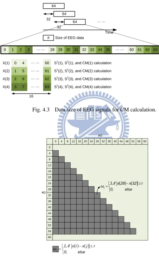
_{( 15 )}

In this thesis, the setting of parameters is m=1, N=16, and r which differs from one another. The calculation of CM in this work is schematically represented below. First, the 64-point of EEG data is divided into 4-vector for computing CM as shown in Fig. 4.3. Second, to take an example from X(1), we calculate j of each square in Fig. 4.4 and Fig. 4.5. Third,

each j is summed up in the S1 in Fig. 4.4, and S2 is calculate in the same way in Fig. 4.5.

Fourth, using Eq. ( 13 ) compute the sub-CM of each vector. Finally, we sum up sub-CM into CM, and the results are depicted in four states as shown in Fig. 4.6. As a result, it is observed that CM can quantify the regularity or complexity of a time series of signals. Because periodic signal components of seizures reduce complexity levels, CM is utilized to analyze the complexity of EEG signals. However, SWS and artifact also show rhythmic patterns, so discrimination ability of CM is reduced. Therefore, to improve the performance of epileptic

(28)

seizure detection, it is required to combine complementary features to CM analysis. Spectral analysis is recruited for this purpose.

0 1 2 3 … … 28 29 30 31 32 33 34 35 … … 60 61 62 63

# Size of EEG data 64 64 64 32 32 Time … … 0 60 1 5 2 6 3 7 4 61 62 63 … … … … … … … … X(1) X(2) X(3) X(4) S1(1), S2(1), and CM(1) calculation S1(2), S2(2), and CM(2) calculation S1_{(3), S}2_{(3), and CM(3) calculation} S1(4), S2(4), and CM(4) calculation 16

Fig. 4.3 Data size of EEG signals for CM calculation.

0 4 8 12 16 20 24 28 32 36 40 44 48 52 56 60 0 4 8 12 16 20 24 28 32 36 40 44 48 52 56 60 x(i) x(j)     else r 32 x 28 x if 0, 1, ωj           else r j x i x if 0, 1, ωj      

(29)

0 4 8 12 16 20 24 28 32 36 40 44 48 52 56 60 0 4 8 12 16 20 24 28 32 36 40 44 48 52 56 60 x(i) x(j) 0 4 8 12 16 20 24 28 32 36 40 44 48 52 56 60 0 4 8 12 16 20 24 28 32 36 40 44 48 52 56 60 x(i) x(j)        





else r 1 j x 1 i x , j x i x max if 0, 1, ω_j                    else r x x , 4 x 0 x max if 0, 1, ωj        4 8

Fig. 4.5 Computation of the S2 value.

Fig. 4.6 Complexity measurement in four behavioral states.

0 2 4 6 8 10 12 14 16 18 20 80 100 120 140 160 W K D ig it iz e d E E G s ig n a l Time(sec) 0 2 4 6 8 10 12 14 16 18 20 0 1 2 3 4 W K C o m p le x it y m e a s u re m e n t Time(sec) 0 2 4 6 8 10 12 14 16 18 20 80 100 120 140 160 SWD D ig it iz e d E E G s ig n a l Time(sec) 0 2 4 6 8 10 12 14 16 18 20 0 1 2 3 4 SWD C o m p le x it y m e a s u re m e n t Time(sec) 0 2 4 6 8 10 12 14 16 18 20 80 100 120 140 160 SWS D ig it iz e d E E G s ig n a l Time(sec) 0 2 4 6 8 10 12 14 16 18 20 0 1 2 3 4 SWS C o m p le x it y m e a s u re m e n t Time(sec) 0 2 4 6 8 10 12 14 16 18 20 80 100 120 140 160 Artifact D ig it iz e d E E G s ig n a l Time(sec) 0 2 4 6 8 10 12 14 16 18 20 0 1 2 3 4 Artifact C o m p le x it y m e a s u re m e n t Time(sec)

(30)

4.1.2 Spectral Analysis

In this thesis, short-term Fourier transform is used to analyze spectral power distribution. It is observed that enormous power of the absence seizure is at the fundamental frequency (Band1 at 7-9 Hz) and at the second harmonic (Band2 at 14-18 Hz) as seen in Fig. 4.7. SWS state contains delta rhythms (Band0) as well as some oscillations at higher frequencies. Artifact state has high power at low and some high frequency bands. Therefore, EEG band powers are combined with CM to improve the performance of epileptic seizure detection.

WK SWD

SWS Artifact

Band1 Band2

Band0

Fig. 4.7 Spectral analysis in four behavioral states.

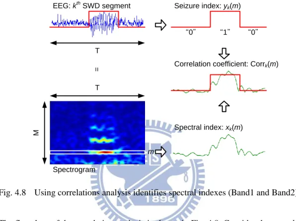
The 64-point fast Fourier transform (FFT) is used to calculate the power of two frequency bands (Band1 and Band2) of spontaneous brain waves because of its well-established implementation in various microprocessors. Fig. 4.7 displays the highest correlations between the power of two frequency bands (Band1 and Band2) and SWDs; therefore, Band1 and Band2 are selected as spectral indexes. To determine spectral indexes to extract an SWD feature adequately, a seizure event (denominated as “1”) is correlated with

(31)

the power of several specific frequency bands by using Pearson's product-moment correlation coefficient. Fig. 4.8 shows that using correlation analysis between seizure event and a specific frequency band identifies effective spectral indexes for seizure detection.

Correlation coefficient: Corrk(m)

M

Spectrogram

EEG: kth SWD segment Seizure index: yk(m)

Spectral index: xk(m) “0” “1” “0” T T = m

Fig. 4.8 Using correlations analysis identifies spectral indexes (Band1 and Band2).

The flowchart of the correlation analysis is shown in Fig. 4.8. Consider there are k SWD segments. SP(t,f) is the spectrogram at time t in frequency f.

1) Define the spectral indexes Xk to be

 

k k X x m            ( 16 ) where

 

SP 1,

 

,SP 2,





, ,SP T,





k k k k x m   m m m _ ( 17 )

(32)

2) Define the seizure index

   

1 , 2 , ,

 

T

k k k k

y     _ ( 18 )

where

 

1, if the state is SWD in time

0, else k t t  _{ }   ( 19 )

3) The correlation coefficient Corrk(m) of the seizure index yk and the spectral index xk is

 



 







 





2





2 k k k k k k k k k x m x m y y Corr m x m x m y y     



( 20 )

4) The averaged correlation coefficient of k segments is

 

K k

 

Corr m C m

k





( 21 )

Fig. 4.9 shows an example of correlations between the spectral index and the seizure index. The selected frequency bands are Band1=8-11 Hz and Band2=17-20 Hz for subject #1. In this project, the sampling frequency Fs is 200 Hz, and the sampled data are N points. The spectral

index n of bands is calculated by the following equation, where Fn is spectral frequency. As a

result, the spectral index of selected frequency bands is n=4 for Band1 and n=7 for Band2 for subject #1.



1



s n F n F N    ( 22 )

(33)

0 5 10 15 20 25 30 35 40 -0.1 0 0.1 0.2 0.3 0.4 0.5 0.6 Frequency(m)(Hz) C o rr e la ti o n C o e ff ic ie n t Band1 Band2

Fig. 4.9 Result of correlation analysis.

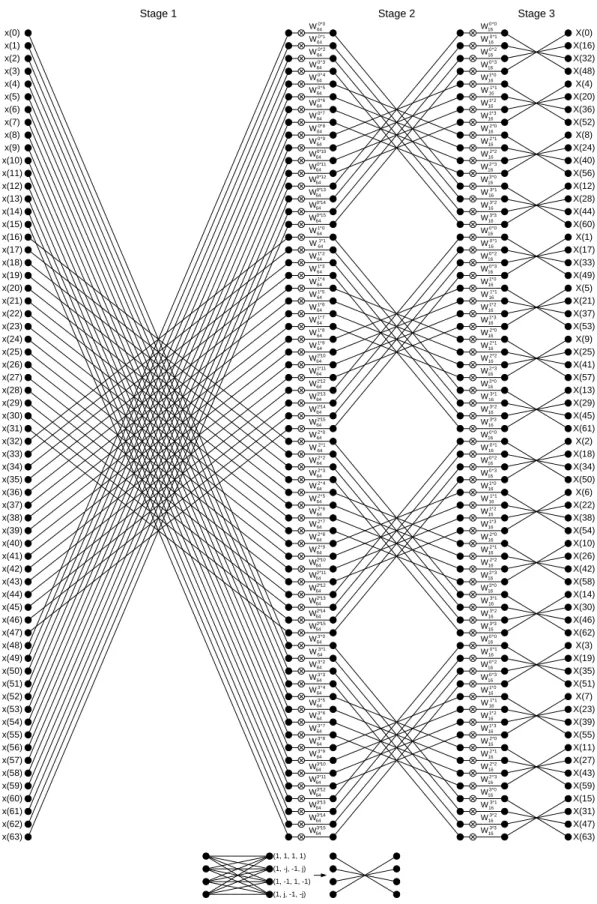
After determining the selected frequency bands, we use 64-point radix-4 FFT to calculate the power of Band1 and Band2 of 64-point EEG signals as shown in Fig. 4.10.

0 1 2 3 … … 28 29 30 31 32 33 34 35 … … 60 61 62 63

# Size of EEG data 64 64 64 32 32 Time … …

(34)

Basically, discrete Fourier transform (DFT) is to compute the sequence X(k) of N complex-valued numbers given another sequence of data x(n) of length N.

 

1

 

0 N kn N n X k x n W   



( 23 ) where 2 , for 0 1 j kn kn _N N W e k N         ( 24 )

The radix-4 decimation-in-time algorithm rearranges the DFT equation into four parts as follows.

 

X k ( 25 )

 

4 1 2 1 3 4 1 1 0 4 2 3 4 N N N N kn kn kn kn N N N N n n N n N n N x n W x n W x n W x n W         















( 26 )

 

4 1 4 1 4 1 4 2 0 0 4 0 2 N N N kn Nk kn Nk kn N N N N N n n n N N x n W W x n W W x n W             _  _  _  _    



4 1 3 4 0 3 4 N Nk kn N N n N W x n W      _  _  



( 27 )

   

 

4 1 0 3 1 4 2 4 N k k k _nk N n N N N x n j x n x n j x n W           _   _  _  _  _ _  __        



( 28 )

Using k1+4k2 to substitute k, we rearrange Eq. ( 28 ) into Eq. ( 29 ). In this algorithm, there are

three stages involving 64-point uniform radix-4 algorithmic processes. The data flow of 64-point radix-4 FFT is shown in Fig. 4.11.





   

1

 

1

 

1 ₁ ₂ 4 1 1 2 4 0 3 4 1 4 2 4 N k k k _nk _nk N N n N N N X k k x n j x n x n j x n W W             __   _  _  _  _ _  __ _          



( 29 )

(35)

x(0) x(1) x(2) x(3) x(4) x(5) x(6) x(7) x(8) x(9) x(10) x(11) x(12) x(13) x(14) x(15) x(16) x(17) x(18) x(19) x(20) x(21) x(22) x(23) x(24) x(25) x(26) x(27) x(28) x(29) x(30) x(31) x(32) x(33) x(34) x(35) x(36) x(37) x(38) x(39) x(40) x(41) x(42) x(43) x(44) x(45) x(46) x(47) x(48) x(49) x(50) x(51) x(52) x(53) x(54) x(55) x(56) x(57) x(58) x(59) x(60) x(61) x(62) x(63) 0 0* 64 W 1 * 0 64 W 2 * 0 64 W 3 * 0 64 W 4 * 0 64 W 5 * 0 64 W 6 * 0 64 W 7 * 0 64 W 8 0* 64 W 9 * 0 64 W 10 * 0 64 W 11 * 0 64 W 12 * 0 64 W 13 * 0 64 W 14 * 0 64 W 15 * 0 64 W 1 * 1 64 W 2 * 1 64 W 3 * 1 64 W 4 * 1 64 W 5 * 1 64 W 6 * 1 64 W 7 * 1 64 W 8 * 1 64 W 9 * 1 64 W 10 * 1 64 W 11 * 1 64 W 12 * 1 64 W 13 * 1 64 W 14 * 1 64 W 15 * 1 64 W 0 * 1 64 W 0 * 2 64 W 1 * 2 64 W 2 * 2 64 W 3 * 2 64 W 4 * 2 64 W 5 * 2 64 W 6 * 2 64 W 7 * 2 64 W 8 * 2 64 W 9 * 2 64 W 10 * 2 64 W 11 * 2 64 W 12 * 2 64 W 13 * 2 64 W 14 * 2 64 W 15 * 2 64 W 0 * 3 64 W 1 * 3 64 W 2 * 3 64 W 3 * 3 64 W 4 * 3 64 W 5 * 3 64 W 6 * 3 64 W 7 * 3 64 W 8 * 3 64 W 9 * 3 64 W 10 3* 64 W 11 * 3 64 W 12 3* 64 W 13 3* 64 W 14 3* 64 W 15 3* 64 W 0 * 0 16 W 1 * 0 16 W 2 * 0 16 W 3 * 0 16 W 0 * 1 16 W 1 * 1 16 W 2 * 1 16 W 3 * 1 16 W 0 * 2 16 W 1 * 2 16 W 2 * 2 16 W 3 * 2 16 W 0 * 3 16 W 1 3* 16 W 2 3* 16 W 3*3 16 W 0 * 0 16 W 1 * 0 16 W 2 * 0 16 W 3 * 0 16 W 0 * 1 16 W 1 * 1 16 W 2 * 1 16 W 3 * 1 16 W 0 * 2 16 W 1 * 2 16 W 2 * 2 16 W 3 * 2 16 W 0 * 3 16 W 1 3* 16 W 2 3* 16 W 3*3 16 W 0 * 0 16 W 1 * 0 16 W 2 * 0 16 W 3 * 0 16 W 0 * 1 16 W 1 * 1 16 W 2 * 1 16 W 3 * 1 16 W 0 * 2 16 W 1 * 2 16 W 2 * 2 16 W 3 * 2 16 W 0 * 3 16 W 1 3* 16 W 2 3* 16 W 3*3 16 W 0 * 0 16 W 1 * 0 16 W 2 * 0 16 W 3 * 0 16 W 0 * 1 16 W 1 * 1 16 W 2 * 1 16 W 3 * 1 16 W 0 * 2 16 W 1 * 2 16 W 2 * 2 16 W 3 * 2 16 W 0 * 3 16 W 1 3* 16 W 2 3* 16 W 3*3 16 W X(0) X(16) X(32) X(48) X(4) X(20) X(36) X(52) X(8) X(24) X(40) X(56) X(12) X(28) X(44) X(60) X(1) X(17) X(33) X(49) X(5) X(21) X(37) X(53) X(9) X(25) X(41) X(57) X(13) X(29) X(45) X(61) X(2) X(18) X(34) X(50) X(6) X(22) X(38) X(54) X(10) X(26) X(42) X(58) X(14) X(30) X(46) X(62) X(3) X(19) X(35) X(51) X(7) X(23) X(39) X(55) X(11) X(27) X(43) X(59) X(15) X(31) X(47) X(63) (1, 1, 1, 1) (1, -j, -1, j) (1, -1, 1, -1) (1, j, -1, -j)

Stage 1 Stage 2 Stage 3

(36)

4.2 Classifier

Three feature indexes (CM and power of Band1 and Band2) are input into a classifier to verify seizure occurrences. In order to implement the proposed seizure detection method on an embedded system, a linear classifier called linear least squares (LLS) [35] is utilized. In mathematics, a system of linear equations is considered over-determined if there are more equations than unknowns. The method of least squares is a standard approach to the approximate solution of over determined systems. The LLS method finds the most approximate linear model which is minimized the mean square error between the system output and the desired output. Because the model’s output is only the weighted sum of three input features, it is suitable for processing on-line system without complicated computation.

Consider an over-determined system

1 , for 1, 2, , n i ij j j y X  i m  



   ( 30 )

of m linear equations in n unknown coefficients, 1, 2, …, n with mn. It can be written in matrix form as yX ( 31 ) where 1 11 1 1 1 , , n n m mn n y x x y X y x x                _{ }  _ _  _{ }             ( 32 )

In this thesis, we let the output of LLS be y, the input of LLS be X, and the weighted coefficient of input be . Such a system usually has no solution, so the goal is instead to find the coefficients  which fit the equations best. The coefficients  can be find by following equations.

(37)

The residual r is the difference between the observed value y and the calculated value X by the model: 1 , for 1, 2, , n i i ij j j r y X  i m   



   ( 33 )

Then the sum of square of the residuals S can be written

2 1 m i i S r  



( 34 )

S is minimized when its gradient vector is zero. The elements of the gradient vector are the

partial derivatives of S with respect to the parameters

1 2 0, for 1, 2, , m i i i j j r S r j n     _   _ _{   }     



_ _ ( 35 )

and the residuals r

i ij j r X      ( 36 )

We use Eq. ( 33 ) and Eq. ( 36 ) in substitution for Eq. ( 35 )

 

1 1 2 0, for 1, 2, , m n i ik k ij i k j S y X  X j n     _  _  _ _{   }   



_



_ ( 37 ) If ˆ minimizes S, we have





1 1 ˆ 2 0, for 1, 2, , m n i ik k ij i k j S y X  X j n     _  _  _ _{   }   



_



_ ( 38 )

Upon rearrangement, the normal equations can be rewritten

1 1 1 ˆ _{, for} _{1, 2,} _, m n m ij ik k ij j i k i X X  X y j n       





( 39 )

The normal equations are written in matrix notation as



T



ˆ T

(38)

The optimal coefficients ˆ can be determined by following equation.





1

ˆ T T

X X X y

   ( 41 )

In training phase, all SWD durations and the non-seizure segments with the length equivalent to the SWDs are selected for the LLS model training. In the non-seizure segments, the ratios of the data corresponding to WK, SWS, and the artifact are 1:1:1. For example, in Fig. 4.12, the ratios of the six data corresponding to SWD, WK, SWS, and the artifact are 3:1:1:1. The inputs Xij of LLS classifier are formed into Eq. ( 42 ). The target value yi is 0 for

non-seizure segments, and 1 for seizure segments. The optimal coefficients ˆ can be determined by Eq. ( 41 ) for each rat through an off-line process.

Seizure Non-seizure

CM0 CM1 CM2 CM3 CM4 CM5

Band10 Band11 Band12 Band13 Band14 Band15 Band20 Band21 Band22 Band23 Band24 Band25

SWD WK SWS Artifact

Fig. 4.12 An example of LLS classifier’s input X.

0 0 0 1 1 1 CM 2 2 2 Band1 Band 2 3 3 3 Const 4 4 4 5 5 5 CM Band1 Band 2 1 1 CM Band1 Band 2 1 1 CM Band1 Band 2 1 1 _ˆ , , CM Band1 Band 2 1 0 CM Band1 Band 2 1 0 CM Band1 Band 2 1 0 Coeff Coeff y X Coeff Coeff          _ _     _ _     _ _ _{ }  _ _        _ _     _ _           ( 42 )

In testing phase, the optimal coefficients ˆ are applied for Eq. ( 43 ), where three features are obtained from testing data. If the output LLS is larger than a threshold (T1 or T2), the input EEG signals is classified as a seizure event.

CM Band1 Band 2 Const

(39)

4.3 EEG Data for Training and Testing

4.3.1 Training Phase

The purpose of training is to determine a fitting model which contains four coefficients and four thresholds for each subject. Fig. 4.13 shows the procedure of training phase. Continuous EEG signals of each rat are recorded for marking and training. After recorded, EEG signals which correspond to seizures (SWD) and non-seizures (WK, SWS, and artifact) are marked by specialist. The marked events as mentioned above are used to extract CM, Band1, Band2, and Band0 values. After that, we start to train eight parameters including four coefficients and four thresholds. The following are the details of EEG data training.

EEG recording

EEG data marking

EEG data training Seizure(SWD) Non-seizure(WK, SWS, Artifact)

Acquire 4-coefficient and 4-threshold

4-coefficient (CM, Band1, Band2, constant) 4-threshold (T1, T2, THsws, TLsws) Off-Line Training Phase in Computer

EEG data selection

LLS 4-coefficient computation

4-threshold search

Fig. 4.13 Procedure of training phase.

First, we randomly select the EEG segments of four states, and the ratios of the segments corresponding to SWD, WK, SWS, and the artifact must be 3:1:1:1 as shown in Fig. 4.14. Second, we execute CM and FFT computation to obtain CM, Band1, Band2, and Band0 values. Third, combined feature substitute the X of Eq. ( 41 ), and desired output substitutes the y of Eq. ( 41 ) like Eq. ( 42 ). Then, the optimal coefficients ˆ can be determined. Fourth,

(40)

the optimal coefficients ˆ are applied for Eq. ( 43 ), where three features are obtained from training data. Then, we search the optimal thresholds from LLS and Band0 values in order to recognize a seizure event. The flowchart of seizure determination is shown in Fig. 4.15, and we test many sets of thresholds in detection rate and false detection rate for finding the most optimal thresholds. 64 64 64 64 64 … … CM CM CM CM CM

Band1 Band1 Band1 Band1 Band1

Band2 Band2 Band2 Band2 Band2

Time # CM Band1 Band2 Feature extraction # # # 64 SWD segment WK segment SWS segment artifact segment 0 0 1 1 1 0 Desired output output of LLS Input of LLS

Band0 Band0 Band0 Band0 Band0 Band0

Fig. 4.14 Feature extraction and LLS classifier training.

TLSWS<Band0 && Band0<THSWS WK SWS Seizure alarm LLS >= T1 LLS >= T2 Y Y Start Y N

(41)

In previous work, four thresholds are obtained by using exhaustive key search. In Fig. 4.16 (a), we do not calculate the distribution of seizure’s and non-seizure’s values of LLS and Band0, and we use every set of 4-threshold to test detection rate and false detection. We need (MN)2 times of iterations to find the best thresholds. As a result, original method wastes a lot of time on parameter determination. To speed up parameter determination, it is proposed that using the mean and the multiples of standard deviation finds four thresholds rapidly. We calculate the distribution of seizure’s and non-seizure’s values of LLS and Band0. According

to the step as mentioned above, we only need

2 M N × m n    

  times of iterations to find the best

thresholds.

The value of LLS … … M times to search T1 value

M times to search T2 value

The value of Band0 … …

N times to search TLSWS value

N times to search THSWS value

… … … … … … … … … … … … The value of LLS

The value of Band0

Mean Standard deviation

M/m times to search T1 value

… … … …

Standard deviation

Mean

M/m times to search T2 value

Mean Standard deviation

… … … …

N/n times to search TLSWS value

… … … …

Standard deviation

Mean

N/n times to search THSWS value

(a) (b)

Fig. 4.16 (a) Original search for 4-threshold, (b) Proposed search for 4-threshold. The following are the steps of the fast parameter determination method. Moreover, the flowchart of fast parameter determination method is depicted in Fig. 4.17.

1) The four coefficients of Eq. ( 43 ) is substituted for optimal coefficients ˆ, and we calculate the LLS value of Eq. ( 43 ).

2) We compute the mean and the standard deviation of actual non-SWD’s LLS value as shown in Fig. 4.18 (a), so T1 can be written





(42)

where i is multiple of standard deviation. We choose a real number to substitute i for calculating T1, and the detection rate of our system is determined in this step.

3) We compute the mean and the standard deviation of actual SWD’s Band0 value as depicted in Fig. 4.18 (a), so THSWS can be written





SWS

TH SWD's Band 0 j  SWD's Band 0 ( 45 )

where j is multiple of standard deviation. We choose a real number to substitute j for calculating THSWS, and the false detection rate is reduced in this step.

4) After executing three steps as mentioned above, we compute the mean and the standard deviation of FP’s LLS value and FP’s Band0 value as shown in Fig. 4.18 (c). T2 and TLSWS can be written





T 2FP's LLS k  FP's LLS ( 46 )





SWS TL FP's Band 0 l  FP's Band 0 ( 47 )

where k and l are multiple of standard deviation. We choose real numbers separately to substitute k and l for calculating T2 and TLSWS, and the false detection rate is also reduced in this step.

5) We test the detection rate and the false detection rate for 4-threshold which is determined by Step(2) to Step(4).

6) Changing the real number of i and j, we iterate form Step (2) to Step (5). In Step (4), we also change the real number of k and l, we iterate form Step (4) to Step (5). Finally, we can select the best threshold from the test in Step (5).

(43)

T1=t1i THSWS=thswsj k<=M/m (5) Calculate Performance End Start to find T1, T2, THSWS,TLSWS i=0, j=0, k=0, l=0 i=i+1 (1) Calculate LLS (2) Calculate T1' T1'=[t11 t12 … t1i … t1(M/m)] (4) Calculate T2' T2'=[t21 t22 … t2k … t2(M/m)] Calculate TLSWS' TLSWS'=[tlsws1 tlsws2 … tlswsl … tlsws(N/n)] (3) Calculate THSWS' THSWS'=[thsws1 thsws2 … thswsj … thsws(N/n)] k=k+1 T2=t2k TLSWS=tlswsj i<=M/m l=l+1 j=j+1 l<=N/n j<=N/n l=0 k=0 j=0 Y N Y N N Y Y N

(44)

FP FP TN TN TN FP Band0 LLS TP TP TP LLS (2) T1 Band0 TN FP TN TN TN TN TP TP TP LLS T1 Band0 (3) THSWS TN TN TN TN TN TN TP TP TP LLS T1 Band0 THSWS (4) TLSWS TN TP FP (4) T2 Actual seizure Actual non-seizure

True Negative: Actual non-seizure, tested non-seizure False Positive: Actual non-seizure, tested seizure True Positive: Actual seizure, tested seizure

(a) (c)

(b) (d)

Fig. 4.18 (a) Original data, (b) Determine T1, (c) Determine THSWS, (d) Determine T2 and TLSWS.

4.3.2 Testing Phase

Fig. 4.19 shows the procedure of testing phase. In testing phase, after the parameters of a seizure detection model, which include 4-coefficient of LLS classifier and 4-threshold of seizure determination, are determined from training phase, the parameters are downloaded to our processor. The seizure detection algorithm as shown in Fig. 4.20 is executed on OpenRISC. After initializing the system, we start to acquire 32-point EEG data. Then, we compute 64-point data of time domain CM and frequency domain FFT. After the CM, Band1, and Band2 values are obtained, LLS value is calculated by Eq. ( 43 ). A seizure alarm is discriminate from normal EEG signals by determining LLS and Band0 values. When the counter reaches “3”; that is, NC equals 3 in Fig. 4.20, a seizure is determined. In the meantime, an enable signal is generated to stimulator in our system.

(45)

Parameters setting from training

On-line seizure controller testing Set 4-coefficient and 4-threshold in OpenRISC

4-coefficient (CM, Band1, Band2, constant) 4-threshold (T1, T2, THsws, TLsws) On-Line Testing Phase in OpenRISC Data acquisition CM and FFT computation LLS computation Seizure determination Calculate 4-feature, LLS value,

and seizure determination

4-feature(CM, Band1, Band2, Band0)

Fig. 4.19 Procedure of testing phase.

TLsws<Band0<THsws LLS>=T1 LLS>=T2 Y N N Y Y WK SWS Counter++ Counter>=NC N Y Detected SWD N Counter=0 Counter=0 Counter=0 32 Data CM FFT LLS Seizure Determination Initialization Y N Detected SWD N Y … … N

(46)

Chapter 5 Design and Implementation

This chapter presents the design and implementation of the proposed low-power BSP, including hardware architecture and firmware.

5.1 The Low-Power Biomedical Signal Processor

The low-power BSP implementation bases on the OR1200 for epileptic seizure control. OR1200 is a 32-bit scalar RISC with Harvard micro-architecture, five stage integer pipeline, memory management units (MMU), and basic DSP capabilities. Supplemental facilities include debug unit for real-time debugging, high resolution tick timer, programmable interrupt controller, and power management support. OR1200 is designed for embedded, portable, and networking applications. Fig. 5.1 (a) shows the block diagram of OR1200.

Because the area is proportional to power consumption, the unnecessary interfaces and modules are removed for optimizing power consumption. The external interfaces of the power management, debug module and interrupt controller are removed. Some modules which consist of the memory management units and the caches are also removed. Furthermore, the instruction and data bus are controlled by an arbiter. Instruction and data bus are merged, so the data bandwidth is reduced. Instruction bus has the highest priority to access bus. The purpose of merged buses is a trade-off between power and execution time. Fig. 5.1 (b) shows the block diagram of the proposed low-power BSP for epileptic seizure control.

(47)

CPU/DSP Data Memory Management Unit Instruction Memory Management Unit Instruction Cache Data Cache W is h b o n e I/ F W is h b o n e I/ F Tick Timer Debug Module Power Module Programmable Interrupt Controller System I/F PM I/F DB I/F INT I/F OpenRISC 1200 CPU/DSP Tick Timer Debug Module Power Module Programmable Interrupt Controller System I/F The proposed low-power BSP

W is h b o n e I /F Arbiter Instruction Wishbone Bus Data Wishbone Bus (a) (b)

Fig. 5.1 (a) Block diagram of OR1200 processor, (b) Block diagram of the proposed low-power BSP.

The proposed BSP is implemented in TSMC 0.18 m complementary–metal–oxide semiconductor 1P6M process and ARM design kit by using cell-based design flow. Fig. 5.2 shows the chip layout and die photo. A total of 104 pads are utilized in this work, which are 71 input/output pads and 33 power pads. The core area is 1.01.0 mm and the chip area is 1.751.75 mm. The maximum operating clock rate is 110.0 MHz at 1.8 V core supply and 3.3 V input/output (I/O) pads supply. The power consumption of core and I/O pads is 0.23 mW/MHz and 0.26 mW/MHz, respectively. One vertical and two horizontal power strips are distributed in the core to reduce voltage drop. The summary of circuit characteristics is listed in Table 5.1.

(48)

(b) (a)

Fig. 5.2 The (a) chip layout and

(b) die photo of the implemented low-power BSP.

Technology TSMC 0.18 m 1P6M Logic Process

Cell Library TSMC SAGE-X Standard Cell Library

Core / Chip Area 10001000 mm2 / 17501750 mm2

Core Supply Voltage / I/O Supply Voltage 1.8V / 3.3V

Maximum Operating Clock Rate 110.0 MHz

Gate Count 60,132

Power Dissipation of Core 0.23 mW/MHz

Power Dissipation of I/O 0.26 mW/MHz

Power Dissipation of Chip 0.49 mW/MHz

(49)

5.2 Firmware Implementation

In brief, the firmware in the low-power BSP consists of three parts, data acquisition, seizure detection, and stimulation pulse generation. Fig. 5.3 shows the flowchart of the main program which comprises seizure detection algorithm and two interrupt service routines (ISRs) for a timer. In previous work, ISR1 also computes S1 and S2, and the timing diagram is depicted in Fig. 5.4 (b). It wastes time on calling subprogram which is S1 and S2 computation, when ISR1 is started up. Moreover, because of the subprogram as mentioned above, the result of previous 32 samples is delayed. As a result, we rearrange main program, and the timing diagram is shown in Fig. 5.4 (a). The result of previous 32 samples is obtained earlier than that of previous work. The following are the details of three sub-programs.

ISR1 ISR2 System Initialization Current 1'st EEG Sample CM FFT LLS Seizure Determination Set Stimulation Flag

Update One EEG Sample Generate 800Hz Pulses S1 and S2 Computation Data Acquisition Y N Y N

Seizure Detection Stimulation Pulse Generation

Previous 32 samples Current 32 samples

Fig. 5.3 Flowchart of (a) data acquisition, (b) seizure detection, and (c) stimulation pulse generation.

(50)

CM computation on previous 32 samples FFT computation on previous 32 samples LLS classification on previous 32 samples Seizure determination on previous 32 samples S1 and S2 computation on current 32 samples Previous 32 samples Current 32 samples Next 32 samples t+32 (b) t-31 t t+63 (a)

Result of previous 32 samples

使用開放式精簡指令集處理器應用於即時偵測失神性癲癇動物模型之軟硬體共同實現

國 立 交 通 大 學

電信工程研究所

碩 士 論 文