虛擬駕駛環境下腦波頻譜與反應時間之關聯

(1)

國

立

交

通

大

學

電機與控制工程學系

碩士論文

虛擬駕駛環境下腦波頻譜與反應時間之關聯

Changes in EEG Power Spectra Correlated with Driving

Performance in Simulated Driving Environment

研究生：陳青甫ˉˉˉ

指導教授：林進燈教授

(2)

(3)

虛擬駕駛環境下腦波頻譜與反應時間之關聯

Changes in EEG Power Spectra Correlated with Driving

Performance in Simulated Driving Environment

研究生：陳青甫 Student: Ching-fu Chen

指導教授：林進燈 Advisor: Chin-Teng Lin

國立交通大學

電機與控制工程學系

碩士論文

A Thesis

Submitted to Department of Electrical and Control Engineering College of Electrical Engineering

National Chiao Tung University in partial Fulfillment of the Requirements

for the Degree of Master

in

Department of Electrical and Control Engineering July 2009

(4)

(5)

虛擬駕駛環境下腦波頻譜與反應時間之關聯

研究生：陳青甫指導教授：林進燈教授國立交通大學電機控制工程學系碩士班

摘要

疲勞駕駛不僅危險，並易造成交通事故，故瞌睡偵測系統的開發已成為駕駛安全上重要課題。本實驗讓受測者在虛擬實境（VR）下，進行事件相關車輛偏移（event-related lane-departure）實驗，實驗中同時量測受測者的腦電波（EEG）訊號，以了解受測者駕車行為反應與腦電波能量頻譜（power spectrum）之關聯。所錄得之腦電波訊號，在去除雜訊後，先以獨立成份分析（ICA）分出不同獨立訊號源，再將這些訊號源產生的腦波以時頻轉換（time-frequency transform）算出其頻譜。將所得頻譜依訊號源經過分群（clustering）並依相對應受測者反應時間排序後，觀察到兩側枕葉區（bilateral occipital）在 alpha 頻帶（band，頻率為 8~12 赫茲）上的腦波

頻譜能量會隨反應時間增加而上升，但若反應時間更長，則其能量會下降；而在theta 頻帶（頻率為4~7 赫茲）的腦波頻譜能量則隨受測者反應時間增加持續而上升。實驗中亦觀察到若受測者反應時間增加，則該受測者通常會出現打瞌睡的行為。因前述腦區之腦波能量改變現象不論實驗中是否提供動態刺激均可觀察到，故該腦區之腦波特徵可用於設計瞌睡偵測器，以保障駕駛人安全。關鍵字：駕駛安全、疲勞駕駛、警覺程度、瞌睡偵測、事件相關車輛偏移實驗、駕駛行為表現、虛擬實境（VR）、腦電波（EEG）、獨立成份分析（ICA）、時頻轉換（Time-Frequency transform）、腦波頻譜

(6)

(7)

Changes in EEG Power Spectra Correlated with Driving

Performance in Simulated Driving Environment

Student: Ching-fu Chen Advisor: Professor Chin-Teng Lin

Department of Electrical and Control Engineering National Chiao Tung University

ABSTRACT

Drowsy driving is a dangerous behavior and often results in a large number of fatal accidents each year; therefore, understanding the neural correlates of drowsy driving is crucial for the design and evaluation of devices for drowsiness detection. This study investigates the relation between spectral features of electroencephalo-graphic (EEG) signals and driving performance. Subjects participated in long-haul simulated driving experiments on a motion platform, during which driving trajectories and 30-channel EEG signals were recorded simultaneously. Driving performance was measured by reaction time (RT) as defined in an event-related lane-departure paradigm. Following artifact rejection on behavioral and EEG data, independent component analysis (ICA) was used to decompose EEG signals into independent brain processes, and power spectra were computed from the activation time course of each independent component. Independent components with similar features, including topographic maps, dipole sources, and power spectra, were then grouped into clusters across subjects.

(8)

oc-reaction time increased and started to decrease as oc-reaction time further increased (> 3 sec); however, theta-band (4-7 Hz) power increased monotonically as reaction time increased. These spectral features were consistent in both motionless and motion conditions. Finally, the results of this study may provide useful information, such as the selection of optimal electrode locations and frequency bands, for the development of drowsiness detection devices.

Index terms: Driving Safety, Drowsy Driving, Vigilance Level, Drowsiness Detection,

Event-Related Lane Departure Paradigm, Driving Performance, Virtual-Reality (VR), Electroencephalographic (EEG) Signals, Independent Component Analysis (ICA), Time-Frequency Transform, EEG Power Spectrum

(9)

誌謝

在完成論文的過程中，我受到很多人的協助；有大家的幫忙協助，才能順利完成這項研究。首先，我要感謝我的家人，並把這份論文獻給他們。我的家人除了讓我在整個過程中不用煩惱生活上的瑣事外，他們更在低潮時給我鼓勵，讓我有動力繼續前行。在此要向我的家人再次表達由衷的感謝。感謝美國加州大學聖地牙哥分校的黃瑞松博士，在整個研究過程中，黃博士十分耐心地指導我，為我釋疑，並仔細檢查研究中的各個步驟。而指導教授——林進燈教授及實驗室的柯立偉博士，除了為提供良好的研究環境不遺餘力外，並指引我研究的方向；同樣是美國加州大學聖地牙哥分校的鍾子平教授和段正仁博士，及交大的曲在雯教授，在研究結果的詮釋上提出不少建議，並指出我的盲點。感謝實驗室的黃騰毅學長在實驗場景上的設計及調整，李昂穎、莊謹譽、葉人慈三位學弟在實驗進行及資料分析上的支援及協助，及鄭仲良學長在實驗技巧和資料提供上給予的幫忙。最後，我要感謝實驗室其他學長姊、同學、學弟妹在資料分析及詮釋上的經驗分享，及實驗室助理在行政事務上的協助，謝謝大家。在此再向幫助過我的各位表達由衷感謝。

(10)

(11)

Acknowledgements

In the process of finishing this research, I received the help from many people. With their help, I can finish this study smoothly. In the beginning, I’d like to make special thank to my dear families and dedicate this thesis to all of them. Because of them, I didn’t have to worry about my livings throughout the whole process; in addi-tion, when I was frustrated, they consoled and cheered me and gave me more strength. I’d like to say “thank you” to all of them. I’d like to thank Doctor Ruey-Song Huang (黃瑞松博士), who instructed me with great patient and scrutinized the pro-cedures for data analysis carefully. I’d also like to thank Professor Ching-Teng Lin (林進燈教授) and Doctor Li-Wei Ko (柯立偉博士) for the help in the great environ-ment in the lab and the insights in the direction of my study, and Professor Tzyy-Ping Jung (鍾子平教授), Doctor Jen-Ren Duann (段正仁博士), and Professor Tzai-Wen Chiu (曲在雯教授) for the suggestions in interpreting results. Moreover, I’d like to thank Teng-Yi Huang (黃騰毅學長) for the programming of experiment envi-ronment, teammates Yang-yin Lee (李昂穎), Chin-yu Chuang (莊謹譽), and Ren-cih Yeh (葉人慈) for the assistances in data analysis and further experiments, and Jong-Liang Jeng for the instructions in skills in conduction experiments and periment data. Finally, I’d like to thank other lab researchers for sharing their ex-periences and other suggestions in their own studies to make this thesis even better, and the assistants in the lab for other helps. Thank you. Thank you very much.

(12)

(13)

Lists of Tables

Table 1: Behavioral Data of Motionless Datasets...23

Table 2: Behavioral Data of Motion Datasets ...34

Table 3: Number of Components in the Identified Clusters ...68

Table A1: Output Frequency Bins ...75

Table A2: Output Time Points ...75

Table A3: Talairach Coordinates of the Frontal Cluster (Motionless Datasets) ...78

Table A4: Talairach Coordinates of the Central Cluster (Motionless Datasets)...80

Table A5: Talairach Coordinates of the Parietal Cluster (Motionless Datasets) ...82

Table A6: Talairach Coordinates of the Left Somatomotor Cluster (Motionless Datasets)...84

Table A7: Talairach Coordinates of the Right Somatomotor Cluster (Motionless Datasets)...86

Table A8: Talairach Coordinates of the Occipital Midline Cluster (Motionless Datasets)...88

Table A9: Talairach Coordinates of the Bilateral Occipital Cluster (Motionless Datasets)...90

Table A10: Talairach Coordinates of the Tangential Occipital Cluster (Motionless Datasets)...91

Table A11: Talairach Coordinates of the Frontal Cluster (Motion Datasets) ...94

Table A12: Talairach Coordinates of the Central Cluster (Motion Datasets) ...96

Table A13: Talairach Coordinates of the Parietal Cluster (Motion Datasets) ...98

Table A14: Talairach Coordinates of the Left Somatomotor Cluster (Motion Datasets) ...100

Table A15: Talairach Coordinates of the Right Somatomotor Cluster (Motion Datasets)...102

Table A16: Talairach Coordinates of the Occipital Midline Cluster (Motion Datasets)104 Table A17: Talairach Coordinates of the Bilateral Occipital Cluster (Motion Datasets) ...106

Table A18: Talairach Coordinates of the Tangential Occipital Cluster (Motion Datasets)...108

(16)

(17)

Lists of Figures

Figure 1: The layout of the screens in the VR environment at Brain Research Center,

National Chiao Tung University...5

Figure 2: A car body mounted on a 6-DOF Steward motion platform...6

Figure 3: A bird’s eye view of the event-related lane-departure paradigm ...7

Figure 4: The layout of electrodes on the EEG caps used in the experiments ...8

Figure 5: The flowchart of data analysis and signal processing ...9

Figure 6: A segment of the driving trajectory in a representative session ...11

Figure 7: An example of artifacts removal of the recorded EEG signals ...13

Figure 8: Topographic maps of ICA decomposition in a representative session. ...16

Figure 9: The procedures of time-frequency transform ...18

Figure 10: The flowchart of computing tonic power spectra. ...19

Figure 11: Cumulative distribution curve of sorted reaction times in the motionless datasets...24

Figure 12: The average scalp maps of eight IC clusters in the motionless datasets. 25 Figure 13: Results of the frontal cluster in the motionless datasets...26

Figure 14: Results of the central cluster in the motionless datasets...27

Figure 15: Results of the parietal cluster in the motionless datasets...28

Figure 16: Results of the left somatomotor cluster in the motionless datasets ...29

Figure 17: Results of the right somatomotor cluster in the motionless datasets...30

Figure 18: Results of the occipital midline cluster in the motionless datasets ...31

Figure 19: Results of the bilateral occipital cluster in the motionless datasets ...32

Figure 20: Results of the tangential occipital cluster in the motionless datasets ...33

Figure 21: Cumulative distribution curve of sorted reaction times in the motion datasets...35

Figure 22: The average scalp maps of eight IC clusters in the motion datasets...36

Figure 23: Results of the frontal cluster in the motion datasets ...37

Figure 24: Results of the central cluster in the motion datasets ...38

Figure 25: Results of the parietal cluster in the motion datasets ...39

Figure 26: Results of the left somatomotor cluster in the motion datasets ...40

Figure 27: Results of the right somatomotor cluster in the motion datasets ...41

Figure 28: Results of the occipital midline cluster in the motion datasets...42

Figure 29: Results of the bilateral occipital cluster in the motion datasets ...43

Figure 30: Results of the tangential occipital cluster in the motion datasets ...44 Figure 31: Cumulative distributions of sorted reaction times in motionless and

(18)

Figure 33: Comparison of the trends of tonic power spectra between motionless and motion conditions of the central cluster ...48 Figure 34: Comparison of the trends of tonic power spectra between motionless and

motion conditions of the parietal cluster ...49 Figure 35: Comparison of the trends of tonic power spectra between motionless and

motion conditions of the left somatomotor cluster ...50 Figure 36: Comparison of the trends of tonic power spectra between motionless and

motion conditions of the right somatomotor cluster ...51 Figure 37: Comparison of the trends of tonic power spectra between motionless and

motion conditions of the occipital midline cluster...52 Figure 38: Comparison of the trends of tonic power spectra between motionless and

motion conditions of the bilateral occipital cluster ...53 Figure 39: Comparison of the trends of tonic power spectra between motionless and

motion conditions of the tangential occipital cluster ...54 Figure 40: Comparison of the trends between “tonic” and “mixed” power spectra of

the frontal cluster...59 Figure 41: Comparison of the trends between “tonic” and “mixed” power spectra of

the central cluster...60 Figure 42: Comparison of the trends between “tonic” and “mixed” power spectra of

the Parietal cluster ...61 Figure 43: Comparison of the trends between “tonic” and “mixed” power spectra of

the left somatomotor cluster ...62 Figure 44: Comparison of the trends between “tonic” and “mixed” power spectra of

the right somatomotor cluster...63 Figure 45: Comparison of the trends between “tonic” and “mixed” power spectra of

the occipital midline cluster ...64 Figure 46: Comparison of the trends between “tonic” and “mixed” power spectra of

the bilateral occipital cluster ...65 Figure 47: Comparison of the trends between “tonic” and “mixed” power spectra of

the tangential occipital cluster ...66 Figure A1: The ICA scalp map of each dataset in the frontal cluster (motionless

datasets) ...76 Figure A2: Tonic power spectra of alert trials in the frontal cluster (motionless

datasets) ...77 Figure A3: The locations of dipoles in the frontal cluster (motionless datasets) ...77 Figure A4: The ICA scalp map of each dataset in the central cluster (motionless

datasets) ...78 Figure A5: Tonic power spectra of alert trials in the central cluster (motionless

(19)

Figure A6: The locations of dipoles in the central cluster (motionless datasets) ...79 Figure A7: The ICA scalp map of each dataset in the parietal cluster (motionless

datasets) ...80 Figure A8: Tonic power spectra of alert trials in the parietal cluster (motionless

datasets) ...81 Figure A9: The locations of dipoles in the parietal cluster (motionless datasets) ...81 Figure A10: The ICA scalp map of each dataset in the left somatomotor cluster

(motionless datasets) ...82 Figure A11: Tonic power spectra of alert trials in the left somatomotor cluster

(motionless datasets) ...83 Figure A12: The locations of dipoles in the left somatomotor cluster (motionless

datasets) ...83 Figure A13: The ICA scalp map of each dataset in the right somatomotor cluster

(motionless datasets) ...84 Figure A14: Tonic power spectra of alert trials in the right somatomotor cluster

(motionless datasets) ...85 Figure A15: The locations of dipoles in the right somatomotor cluster (motionless

datasets) ...85 Figure A16: The ICA scalp map of each dataset in the occipital midline cluster

(motionless datasets) ...86 Figure A17: Tonic power spectra of alert trials in the occipital midline cluster

(motionless datasets) ...87 Figure A18: The locations of dipoles in the occipital midline cluster (motionless

datasets) ...87 Figure A19: The ICA scalp map of each dataset in the bilateral occipital cluster

(motionless datasets) ...88 Figure A20: Tonic power spectra of alert trials in the bilateral occipital cluster

(motionless datasets) ...89 Figure A21: The locations of dipoles in the bilateral occipital cluster (motionless

datasets) ...89 Figure A22: The ICA scalp map of each dataset in the tangential occipital cluster

(motionless datasets) ...90 Figure A23: Tonic power spectra of alert trials in the tangential occipital cluster

(motionless datasets) ...91 Figure A24: The locations of dipoles in the tangential occipital cluster (motionless

(20)

...93 Figure A27: The locations of dipoles in the frontal cluster (motion datasets) ...93 Figure A28: The ICA scalp map of each dataset in the central cluster (motion

datasets) ...94 Figure A29: Tonic power spectra of alert trials in the central cluster (motion datasets)

...95 Figure A30: The locations of dipoles in the central cluster (motion datasets)...95 Figure A31: The ICA scalp map of each dataset in the parietal cluster (motion

datasets) ...96 Figure A32: Tonic power spectra of alert trials in the parietal cluster (motion datasets)

...97 Figure A33: The locations of dipoles in the parietal cluster (motion datasets)...97 Figure A34: The ICA scalp map of each dataset in the left somatomotor cluster

(motion datasets) ...98 Figure A35: Tonic power spectra of alert trials in the left somatomotor cluster

(motion datasets) ...99 Figure A36: The locations of dipoles in the left somatomotor cluster (motion datasets)

...99 Figure A37: The ICA scalp map of each dataset in the right somatomotor cluster

(motion datasets) ...100 Figure A38: Tonic power spectra of alert trials in the right somatomotor cluster

(motion datasets) ...101 Figure A39: The locations of dipoles in the right somatomotor cluster (motion

datasets) ...101 Figure A40: The ICA scalp map of each dataset in the occipital midline cluster

(motion datasets) ...102 Figure A41: Tonic power spectra of alert trials in the occipital midline cluster (motion

datasets) ...103 Figure A42: The locations of dipoles in the occipital midline cluster (motion datasets)

...103 Figure A43: The ICA scalp map of each dataset in the bilateral occipital cluster

(motion datasets) ...104 Figure A44: Tonic power spectra of alert trials in the bilateral occipital cluster

(motion datasets) ...105 Figure A45: The locations of dipoles in the bilateral occipital cluster (motion datasets)

...105 Figure A46: The ICA scalp map of each dataset in the tangential occipital cluster

(motion datasets) ...106 Figure A47: Tonic power spectra of alert trials in the tangential occipital cluster

(21)

(motion datasets) ...107 Figure A48: The locations of dipoles in the tangential occipital cluster (motion

(22)

(23)

Abbreviations

EEG: electroencephalographic ICA: independent component analysis IC(s): independent component(s)

RT: reaction time (the reaction time in a trial)

RTs: reaction time (the reaction time in the trials in a group) VR: virtual reality

LDWS: lane departure warning system ESC: electronic stability control EOG: electrooculography HRV: heart-rate variability DOF: degree of freedom

(24)

(25)

Chapter I Introduction

Drowsy driving is a dangerous behavior and results in a large number of fatal accidents each year. When the drivers are drowsy, they have 1) impaired reaction time (RT), judgment, and vision, 2) problems with information processing and short-term memory, 3) decreased performance, vigilance and motivation, and 4) increased moodiness and aggressive behaviors [1]; in addition, they also exhibit dangerous behaviors like running off the road, crossing the center line, or wandering into other lanes or onto the shoulder during drowsy periods [2]. It was reported that in 2008, 54% of adult drivers in the US felt drowsy while driving a vehicle, and 28% of them actually fell asleep at the wheel; moreover, of those who had nodded off, over 50% said they have done so at least once a month [3]. In order to improve driving safety and reduce casualties, it is of great importance to study the neural correlates of drowsy driving, develop devices for monitoring the driver’s vigilance state, and provide timely and effective feedback to the driver.

Several techniques have been developed for drowsiness detection. One of them monitors the driver’s behavior or the vehicle’s lane position, such as the lane-departure warning system (LDWS) [4][5], and other techniques monitor the driver’s physiological activities such as heart-rate variability (HRV) and electroocu-lography (EOG) [6]. The former mainly integrates image-processing based methods to detect lane marking (boundary) and monitor the driver’s activities such as yawn-ing, head positions, or eye blink duration via optical sensors or video cameras [7][8]; however, image- or video-based techniques are sensitive to external weather con-ditions (e.g., rain or snow) and the driver’s posture inside the car. Although the monitoring of physiological signals, such as HRV and EOG, does have the same

(26)

physiological signals is low, making them less effective in the tracking of vigilant states. Among other physiological signals, electroencephalography (EEG) is the most direct and effective measures of vigilant states; however, EEG signals are usually recorded from dozens of scalp electrodes and sampled at 100-500 Hz, which is less viable for on-line signal processing. Owing to the advances in signal acquisition devices and computer speed, recently, real-time analysis and automatic detection of EEG patterns of drowsiness have become more viable [9][10][11].

Numerous studies have suggested that changes in EEG power spectra are re-lated to vigilance and drowsiness. For example, Beatty et al. demonstrated aug-mented occipital theta activities when the radar operators were less vigilant [12]. Huang et al. demonstrated tonic EEG power increase in low-frequency bands in the occipital cortex during high-error periods in a continuous tracking task [13], and they also demonstrated similar tonic EEG power increase in low-frequency bands in the occipital cortex in simulated driving experiments [14]. In addition, Lin et al. demon-strated the correlation between alpha and theta band power and driving error, de-fined as mean deviation from lane center in each moving window [9][15], in a vir-tual-realty (VR) environment. To this day, most studies on drowsy driving have conducted experiments in static laboratory setting; however, in the real world, driv-ers receive kinesthetic stimuli, e.g. vibration on the road, in addition to visual and auditory stimuli. It does not know the effect of kinesthetic stimuli on the EEG power spectra and the accuracy of drowsiness detection, but conducting experiments on the road could be costly and dangerous to the subjects; hence, a dynamic laboratory setting, e.g. a VR environment with a motion platform, is necessary in investigating this issue.

In this study, subjects participated in simulated nighttime driving experiments on a motion platform in a well-controlled VR-based environment [9][15]. An

(27)

event-related lane-departure paradigm [16][17] was used to continuously monitor the subjects’ arousal states, as measured by reaction time to perturbing events on the road. Subjects participated in different sessions, during which the motion plat-form was active (motion condition) or inactive (motionless condition), and their driving trajectories, behavioral responses, and 30-channel EEG signals were re-corded simultaneously. Independent component analysis (ICA) was used to de-compose the 30-channel EEG signals into temporally independent processes, whose sources originated from multiple brain regions, and power spectra were computed from the activation time course of each independent component. Finally, independent components with similar features, such as topographic maps, dipole sources, and power spectra, were grouped into clusters across subjects.

This study aims to 1) identify independent brain processes in different cortical regions whose EEG power spectral changes were related or not related to drowsi-ness, 2) find the trends of different frequency bands in EEG power spectra from alertness to drowsiness across subjects and sessions, and identify frequency bands that are most suitable for drowsiness detection, and 3) compare the above trends in motionless and motion conditions, and find the influence of kinesthetic inputs on EEG power spectra. Finally, the results of this study may provide insights into the design and assessment of drowsiness detection systems for real-life driving.

(28)

(29)

Chapter II Experiment Design and Setup

2.1 VR-Based Driving Simulator and Steward Motion Platform

Simulated driving experiments were conducted in a VR-based driving simulator. A real car body was mounted on a six degree-of-freedom (DOF) Steward motion platform (Figure 1 and Figure 2), which simulated the vibration caused by uneven road surface as well as kinesthetic force during real-life driving. Seven video pro-jectors were used to generate the 360-degree VR scene of night-time driving in a darkened room. This setup provided the subjects with immersive environment and enables the experimenters to control the experiment in a different room.

Figure 1: The layout of the screens in the VR environment at Brain Research Center (BRC), National Chiao Tung University (NCTU). The texts indicate the position of the screens.

(30)

Figure 2: A car body mounted on a 6-DOF Steward motion platform.

2.2 Event-Related Lane-Departure Paradigm

The event-related lane departure paradigm [16][17] was implemented in the VR-based driving simulator using WorldToolKit (WTK) R9 Direct and Visual C++. The paradigm was designed to quantitatively measure the subject’s reaction time to perturbations during continuous driving. Figure 3 shows a bird’s eye view of this task. In this setup, every a few seconds, the car is programmed to randomly drift to the left or right out of a cruising lane with equal probability. Without these lane-departure events, the subject might fall asleep while the car continues to move straight in the lane without deviation in a driving simulator, making it difficult to objectively monitor the subject vigilance level. Following each deviation, subjects were required to steer the cars back to the approximate center of the cruising lane as quick as possible using the steering wheel, and were instructed not to make fine adjustment to the position of the cars and hold on to the wheel after the car returns to the center of the cruising lane.If the subject does not respond promptly, the vehicle will eventually hit the virtual curb on either side without crashes and continue to move along the curb

(31)

even the subject falls asleep. Such experimental design allows the observation of continuous transition from complete alertness to deep drowsy states.

Each lane-departure event is defined as a “trial” which includes three critical moments: “deviation onset” is the moment when the car starts to drift away, “re-sponse onset” represents the moment when the subject perceives the drift and be-gins to steer the cars back to the cruising lane, and “response offset” is the moment when the car returns to the center of the cruising lane, and the subject ceases to rotate the steering wheel. The next lane-departure event occurs again 5~10 sec after the “response offset.” The reaction time is defined as the interval between de-viation onset and response onset in a trial.

Figure 3: A bird’s eye view of the event-related lane-departure paradigm. Figure recreated with per-mission from [16][17].

In order to test the effect of kinesthetic inputs on brain activities and drowsiness, subjects participated in “motionless” and “motion” sessions on different days. The 6-DOF motion platform generated kinesthetic stimuli only in the “motion” sessions. In the “motionless” sessions, the platform was stationary, and no kinetic stimuli were given to the subjects.

2.3 Subjects

(32)

None of them reported psychiatric or sleep disorders. Subjects were given instruc-tion on how to respond to the events before participating in the experiment for the first time. All subjects have participated in the “motionless” session, and seven of them also participated in the “motion” session.

2.4 EEG Recording

The EEG data were recorded at 500 Hz sampling rate from an electrode cap (Neuromedical Supplies 32-channel Quik-Cap) based on the international 10-20 system [18] using a NeuroScan NuAmps amplifier with a band-pass filter (0.1 to 50 Hz). Two reference channels, A1 and A2, were placed on the left and right mastoids, respectively. The impedance of each electrode was ensured to be less than 5k ohms before the EEG acquisition began.

Figure 4: The layout of electrodes on the EEG caps used in the experiments. The blue electrodes are the ones in the international 10-20 system, and the green ones are additional electrodes on the cap.

(33)

Chapter III Data Analysis

In this study , all data analyses and signal processing were implemented by scripts running in MathWorks MATLAB (R2007a) and the EEGLAB Toolbox (version 5.03) developed by the Swartz Center for Computational Neuroscience, the Univer-sity of California San Diego (UCSD) [19]. Figure 5 shows the flowchart of data analysis and signal processing.

Raw EEG data _{and behavioral data}Integration of EEG 0.5 Hz high pass _filter

Artifact Removal (EEG and behavioral data) ICA decomposition

Clustering Component re-_selection Dipole fitting

250 Hz down-sampling 50 Hz low pass filter

Epoch extraction

Computation of tonic power spectra

(by DFT)

Figure 5: The flowchart of data analysis and signal processing.

3.1 Integration of EEG and Behavioral Data

During each experiment, the stimulus computer that generated the VR scene recoded the trajectories of the car as well as the events with time points in a “log” file. The stimulus computer also sent synchronized triggers (which were also recorded in the “log” file) to the Neuroscan EEG acquisition system. At the same time, the Neuroscan system recoded the EEG data with the time stamps of those trigger in an “ev2” file. Since the numbers of time points in both recorded files were different, the first step was to integrate these two files into a new file with aligned event timing and behavioral data. The new event file was then imported by EEGLAB in MATLAB.

(34)

3.2 Epoch Extraction

An epoch is a segment of multi-channel EEG signals time-locked to a specific type of behavioral event. Since there may be more than one event in a trial, the continuous EEG signals in a trial can be extracted into different types of epochs. In order to observe the fluctuation in EEG signals to specific events, the continuous 30-channel EEG signals were extracted into eight-second epochs, time-locked to 1 sec before and 7 sec after each deviation onset.

The “tonic” and “phasic” activities in the recorded data are defined as below [13]. The “tonic” activities in EEG data refer to the longer-term changes in baseline arousal levels. In this study, tonic activities were measured from the cruising period before the deviation onset in each epoch. The “phasic” EEG activities refer to tran-sient event-related brain dynamics time-locked to the deviation onset or response onset/offset.

3.3 Artifact Removal

3.3.1 Removal of Behavioral Artifacts

Two types of abnormal trials in the recorded behavioral data (vehicle trajecto-ries and RTs) were rejected before further analysis. First, those trials with RTs shorter than 0.3 sec were rejected due to the subject’s unintentional responses or the jitters of the steering wheel. Second, when the car returned to the lane center, the trajectories in some trials exhibited “overshoot” or zigzag patterns, making it dif-ficult to clearly define the exact timing of response offset, and thus hard to interpret EEG data; therefore, those trials that did not show “flat” trajectories between the current response offset and the next deviation onset were rejected. Figure 6 dem-onstrates the removal of abnormal trials in behavioral data. Trials 163 and 164 show typical patterns of trajectory of a lane-departure event and were included in the data

(35)

analysis, and trials 159, 160, and 162 were rejected because the subject continued to turn the wheel after response offsets (as indicated in blue dots). In some trials, the steering wheel was not turned into the exact central position (zero angle) after the subject cease to steer, but the computer program misinterpreted the nonzero angle as rotation and made the car continue to drift. For example, trial 161 shows a linear drift during the pre-deviation period, which could be assumed that the subject was not actually steering, and thus this trial was not rejected.

Figure 6: A segment of the driving trajectory in a representative session. X- and y- axes: experiment duration (in seconds) and the lane position of the car (in units), respectively; gray curve: driving trajectory; red, green, and blue dots: driving events: deviation onsets, response onsets, and response offsets, respectively; vertical dotted lines: the beginning of each epoch (one second before deviation onset); numbers below the red dots: indices of trials (red: rejected trial; blue: remained trials after artifact removal) and corresponding RTs (black).

(36)

3.3.2 Removal of EEG Artifacts

In this study, the event-related lane departure task required frequent manual responses using the steering wheel, and sometimes involved body movements to counterbalance with the forces of motion platform during “motion” sessions. These movements often resulted in severe noise in the EEG signals. In addition, a few electrodes lost skin contacts in some periods or throughout the experiment and re-sulted in signals with extreme values in the recorded data. These artifacts could not be dissociated from other brain processes using independent component analysis (ICA), and must be removed before further analysis. Figure 7 demonstrates an example of artifact removal on the recorded EEG data. The following criteria were applied to artifact removal in EEG data: 1) channels with extreme values due to poor skin contact throughout the entire or most parts of the session, and 2) epochs with severe fluctuations across most EEG channels. In Figure 7, epochs 154-156 were rejected due to large fluctuations in channels Fp1, Fp2, F3, and F4; in addition, epoch 158 was rejected because it not only showed large fluctuations on channels Fp1, Fp2, F3, and F4, but also showed widespread noise across all channels.

(37)

Figure 7: An example of artifacts removal of the recorded EEG signals. This figure is a screen snap-shot of the eegplot() function in the EEGLAB toolbox. Horizontal and vertical axes: latency of epochs (in milliseconds, 0: deviation onset of each epoch) and channels, respectively; hori-zontal traces: the recorded EEG signals; vertical lines: deviation onset, response onset, re-sponse offset, and boundaries of epochs; numbers on top: trial indices (horizontal) and event types (vertical).

3.4 Independent Component Analysis (ICA)

3.4.1 Background and Algorithm of Independent Component Analysis

ICA algorithms are a family of related methods for unmixing linearly mixed signals using only recorded time course information (that is, “blind” to detailed models of the signal sources as required by earlier signal processing approaches) [20]. Four main assumptions underlie ICA decomposition of EEG time series: 1) signal conduction times are equal, and summation of currents at the scalp sensors

(38)

source activations are temporally independent of one another across the input data, and 4) statistical distributions of the component activation values are not Gaussian [21]. Given a matrix, W, a vector w, a random vector, x =

[

x K1 xN

]

T , and the linear transform, u= Wx+w , the objective of ICA decomposition is to find the elements in

[

]

T N

u u K1 =

u are statistically independent. ICA imposes that the multivariate prob-ability density function (p.d.f.) of u factorized as

( )

∏

( )

= = N i i u u f f _i 1 u

u , and makes the

mutual information between the ui go to 0: I

(

ui,uj

)

=0∀i,j. In Informax ICA, which

was adopted in this study, the input signals are scaled and shifted to make each of the unknown independent components, u_i , have the same form of cumulative density function (c.d.f.) with the form Fu

( )

u . Next, ICA is performed by maximizing

the entropy H(y) of a non-linearly transform vector y =F_u(u) and thus yields sto-chastic gradient ascent rules for adjusting W and w:

[ ]

W yx y W_∝ 1₊ ˆ ,_Δ _∝ ˆ Δ T − T w (1) where yˆ =

[

yˆ1KyˆN

]

T, and i i i i u y y y ∂ ∂ ∂ ∂ = ˆ [which if y F=

( )

u ]

( )

i u i u u F u f ∂ ∂ = (2)

Instead of using the original c.d.f. of the original signals, the applied c.d.f. in ICA training is ₌

(

1₊ −ui

)

−1

i e

y ; henceforth, yˆ_i ₌1₋2y_i and thus resulting a simple form in this algorithm. These results were obtained even though the p.d.f. of the original signals may not exactly match by the gradient of the logistic function [22].

(39)

3.4.2 Independent Component Activations and Topographic Maps

After artifact rejections, the remained channels and epochs were concatenated into a matrix, x, of size [channels × epochs] and subjected to ICA decomposition using the runica() function of the EEGLAB toolbox. ICA finds an “unmixing” ma-trix, W, which decomposes or linearly unmixes the multi-channel EEG data, x, into a sum of maximally temporally independent and spatially fixed components u, where

u = Wx. Each row of the output data matrix, u (or rows of icaact in the EEGLAB dataset), is the activation time course of each independent component. Each col-umn of the inverse of matrix, W (or icawinv in the EEGLAB dataset), indicates the activation weights distributed across electrodes for each independent component, which can be rendered as a two-dimensional (2-D) topographic map on the scalp.

Figure 8 shows 2-D topographic maps of 30 independent components in a rep-resentative session. Components 2, 3, 4, 6, 7, 8, 9, 10, 11, 14, 18, and 21 are con-sidered as potentially related to brain processes, and others are concon-sidered non-brain artifacts (blinks, eye movements, muscle artifacts, single-channel noise, etc.).

(40)

Figure 8: Topographic maps of ICA decomposition in a representative session.

3.5 Dipole Fitting

Dipole fitting is one of the methods to solve the inverse problem: given an EEG scalp distribution of activity observed at given scalp electrodes, any number of brain source distributions can be found that would produce it [23]. After applying ICA de-composition, many i have scalp maps that nearly perfectly match the projection of a single equivalent dipole on the cortex, and this finding is consistent with their pre-sumed generation via partial synchrony of local field potential (LFP) processes within a connected domain or patch of cortex. The problem of finding the location of a single equivalent dipole generating a given dipolar scalp map is well posed; however, the location of the equivalent dipole for synchronous LFP activity in a “cortical patch” will in general not be in the center of the active cortical patch,

(41)

espe-cially the patch is radially oriented (e.g. on a gyrus, thus aimed toward the super-vening scalp surface), the equivalent dipole location tends to be deeper than the cortical source patch [23]. In this study, the dipole source location of each inpendent component was estimated using the resulting weight matrix of ICA de-composition and the 3-D positions of electrodes. Dipole fitting was implemented using the dipfit plugin in EEGLAB, which finds the optimal dipole location and moments (vectors) that maximally account for the independent component activities with minimum residual variance.

3.6 Computation of Tonic Power Spectra

3.6.1 Time-Frequency Transform

Time-frequency transform is a spectrotemporal decomposition technique that evaluates event-related perturbations in the power spectra (as well as phase and coherence perturbations; not discussed in this study) of single-channel EEG signals or activation time courses of single IC [19]. Figure 9 shows the procedure of time-frequency transform. For each single-channel epoch, the time series are chronically divided into designated numbers of overlapped sub-windows, and the power of each sub-window is then computed by discrete Fourier transform (DFT) using timefreq() function in EEGLAB and fft() function in MATLAB in this study. Finally, a matrix with size [frequency bins × time windows] was obtained for each epoch. The same procedures were applied to all epochs for all EEG channels or IC activations.

(42)

EEG signal or Component activation (-1~0 sec) EEG signal or component activation (-.992~-.484 sec) EEG signal or Component activation (-.988~-.480 sec) EEG signal or Component activation (-.984~-.476 sec) …… EEG signal or Component activation (-.504~.004 sec) DFT or wavelet DFT or wavelet DFT or wavelet …… DFT or wavelet

Power of this signal

(-.992~-.484 sec)

(-.988~.480 sec)

(-.984~.476 sec)

……

(-.504~.004 sec)

Figure 9: The procedures of time-frequency transform of a single-trial and single-channel EEG sig-nals or ICA activation time courses in an epoch. In this research, time-frequency transform was applied only on ICA component activations and using DFT to compute power spectra. Assume this epoch is -1~0 sec (0: deviation onset), and the output is set to 100 time points. The inter-vals of each sub-window were reported by the function timefreq().

3.6.2 Tonic Power Spectra

The goal of this study is to investigate the relation between the changes in tonic EEG power spectra of independent component activations and the fluctuation of driving performance (as measured by reaction time). In order to minimize the effects of phasic EEG power fluctuations during lane departure events, tonic power spectra were computed only from the cruising period before each deviation onset [14]. Figure 10 shows the procedures for computing tonic power spectra, spectral nor-malization, and statistical tests. For each subject (session), logarithmic (log) tonic

(43)

power spectra were computed from a 1-sec window before the “deviation onset” in each 8-sec epoch extracted from each IC activation time courses using DFT (win-dow size: 256 ms; 44 frequency bins between 2.93 and 44.92 Hz, the 2.93-Hz bin was excluded in plotting power images since this frequency bin was beyond the range in this study; 100 time steps between -742.976 and -253.204 sec where 0 sec: deviation onset). The average power spectra were then obtained by averaging across time points to get a mean baseline. Detailed output frequency bins and time points are shown in Table A1 and Table A2).

For each IC of each subject, the tonic power spectra of all epochs (trials) were sorted by their RTs, and then normalized by subtracting the mean power spectra of the “alert trials” with the shortest RT (first 10% of all RT-sorted trials). In this study, the mean power spectra of the alert trials are defined as the “alert baseline power spectra.” Finally, moving average (window size: 10% of total trials; stepping at one trial) was applied to the sorted, normalized power spectra. A two-tailed t-test (ttest2() function in MATLAB) was used to assess if the mean power spectra in each moving window was statistically different from those of the alert trials (p < 10-4, corrected with a Bonferroni multiple comparison method).

(44)

3.7 Independent Component Clustering

3.7.1 Clustering and Re-Selection of Independent Components

In order to characterize the common pattern of spectral activities of similar ICs from different subjects and sessions, these ICs were manually grouped into several IC clusters according to their 2-D topographic maps. Next, initial clustering results were further refined iteratively based on dipole source locations and alert baseline power spectra of ICs in each IC cluster. Components that showed abnormal pat-terns in their topographic maps, dipole source locations, or power spectra deviated from the cluster’s mean were considered outliers. These outliers were rejected from the cluster, and the mean alert baseline power spectra were recomputed from the remaining components in the cluster. In this study, eight IC clusters of brain-related processes were obtained.

3.7.2 Group Trend of Tonic Power Spectra

In order to find the group trend of tonic power spectra, all trials (epochs) in the same IC cluster were grouped and sorted by reaction time, which was used as a common behavioral index to compare the EEG power spectra at similar alertness levels across subjects. The procedures for computing group tonic power spectra from clustered data and statistical tests were slightly different from those applied to single-subject data. In single-subject data, the power spectra of each trial were normalized by the mean power spectra of “alert trials” in the same subject; in the clustered data, the power spectrum of each trial in a moving window was normalized by the mean power spectra of alert trials from its original session, not the mean power of “alert trials” in this cluster. For example, if a trial was from session 3, the power spectra of this trial were normalized by the alert baseline power spectra in that session. In single-subject data, the significance level was estimated by

(45)

com-paring the mean power spectra of trials in a moving window with the alert baseline power spectra from the same session; in the clustered data, the significance level (p <10-10_{, corrected) was estimated by comparing the mean power spectra of trials}

from multiple sessions in a moving window with the weighted baseline (alert) power spectra from the trials’ original sessions. For example, in a moving window with trials 30% from session 1, 30% from session 3, and 40% from session 5, the significance level of this window was estimated by comparing its mean power spectra with the weighted baseline (alert) power from sessions 1, 3, and 5 in consideration of the proportion of trials.

(46)

(47)

Chapter IV Results

4.1 Motionless Datasets

4.1.1 Behavioral Data

Table 1 shows the distribution of behavioral data of individual subjects in the “motionless” condition. The shaded rows show the numbers of trials remained after EEG and behavioral artifact removal. Subjects are sorted in descending order by their drowsiness levels, defined as the percentage of remained trials with RT > 3 sec. In total, 48.66% of original trials in all subjects remained due to severe artifacts in the driving experiments. The car drifted to the left (right) in 49.68% (50.32%) of all the remained trials.

TABLE 1:BEHAVIORAL DATA OF MOTIONLESS DATASETS

Subject Index Trials Data Length (sec)* Trials Re-mained (%)** Min. RT (sec) Max. RT (sec) Avg. RT (sec) SD of RT (sec) Med. of RT (sec) Trials w. RT > 3 sec (%) Dev. to Left (%) 437 6552.12 -- 0.02 110.52 6.09 9.93 2.06 43.71 48.05 s40_070207 222 -- 50.80 0.38 46.37 7.61 9.37 3.38 52.70 45.95 568 6353.32 -- 0.02 49.75 2.16 3.43 0.87 21.13 52.11 s44_070325 223 -- 39.26 0.58 49.75 2.74 4.74 0.84 26.91 41.70 592 6918.08 -- 0.02 109.35 3.09 5.98 1.19 25.00 55.24 s36_061221 336 -- 56.76 0.64 32.15 3.38 4.74 1.24 26.49 54.46 548 6514.88 -- 0.05 628.43 3.45 26.98 1.25 23.54 51.09 s42_070105 197 -- 35.95 0.62 66.26 2.81 5.29 1.50 26.40 50.76 533 6304.28 -- 0.02 40.17 2.94 4.23 1.39 19.14 45.03 s01_061102 287 -- 53.85 0.62 40.17 3.24 4.69 1.35 21.60 44.95 555 5968.00 -- 0.02 56.98 2.44 5.21 0.79 15.32 52.61 s35_070322 195 -- 35.14 0.47 56.98 2.33 6.15 0.73 12.82 60.00 550 7301.76 -- 0.02 30.79 3.16 3.89 1.90 25.64 49.09 s32_061031 250 -- 45.45 0.64 6.64 1.85 0.84 1.67 10.40 48.00 716 6592.20 -- 0.10 8.46 1.22 1.12 0.88 6.42 52.37 s05_061101 402 -- 56.15 0.55 8.01 1.31 1.24 0.90 7.71 50.00

(48)

670 6353.32 -- 0.02 10.65 1.12 1.05 0.75 5.82 49.55 s41_061225 282 -- 42.09 0.32 8.62 1.17 1.15 0.74 7.45 47.16 566 6231.08 -- 0.03 11.23 1.78 1.35 1.35 10.95 48.06 s31_061103 272 -- 48.06 0.72 8.68 1.61 1.16 1.22 7.35 47.43 6363 -- -- 0.02 628.43 2.46 9.02 1.05 17.32 50.32 All subjects 3096 -- 48.66 0.32 66.26 2.50 4.51 1.05 17.31 49.68

Note: shaded areas: distribution of the trials remained after artifacts removal. *: original datasets. **: datasets after artifacts removal.

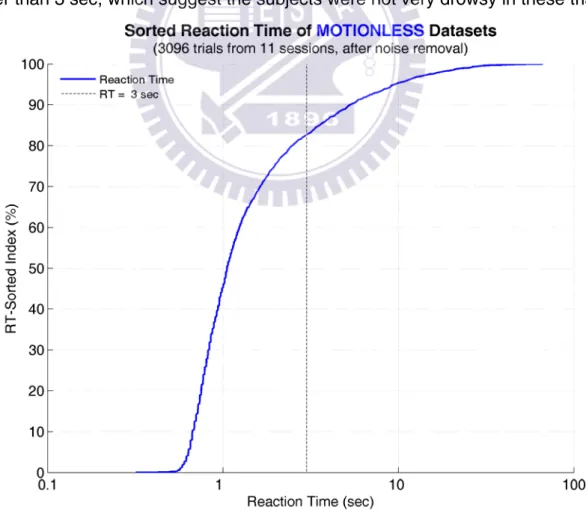
Figure 11 shows the cumulative distribution of sorted reaction time across subjects in the “motionless” datasets. The x- and y- axes are reaction time (in log scale) and percentage of RT-sorted index, respectively, and the vertical dashed line indicates 3-sec RT. The curve shows an approximate bi-linear distribution of RTs (when the x-axis is plotted in linear scale). Only 20% of all remained trials have RTs longer than 3 sec, which suggest the subjects were not very drowsy in these trials.

(49)

4.1.2 Clustered Scalp Maps and Dipole Locations

Eight clusters of independent components with dipole sources located in the frontal, central, parietal, somatomotor, and occipital regions were identified based on their scalp maps from the results of ICA decomposition. The average scalp maps of these IC clusters are shown in Figure 12. Figure A1-Figure A24 show the scalp maps, and Table A3-Table A10 summarize the Talairach coordinates of each dipole in the remaining clusters.

Figure 12: The average scalp maps of eight IC clusters in the motionless datasets.

4.1.3.1 The Frontal Cluster

(50)

trends of tonic power changes in four frequency bands. The power image and traces in Figure 13 D and E, respectively, show about 1~2 dB increase in the theta band when the mean RTs are longer than 1.88 sec, and such increase shifts to the lower frequencies when RTs further increase and become significant (p < 10-10, two-sampled t-test, corrected) when RTs are longer than 6.67 sec.

Figure 13: Results of the frontal cluster in the motionless datasets. A: the average scalp map of all IC in the cluster, B: mean power spectra of alert trials in each dataset and cluster average (blue trace), C: dipole locations (yellow dot: cluster average), D: the moving averaged power image (x-axis: RT-sorted index in percentage and the corresponding reaction time in seconds; y-axis: frequency in Hz; regions inside contour: p < 10-10, two-tailed t-test, corrected for multiple com-parison), and E: trends of mean tonic power in four frequency bands (extracted from D; x-axis: RT-sorted index and the corresponding reaction time in seconds; y-axis: power increase in dB).

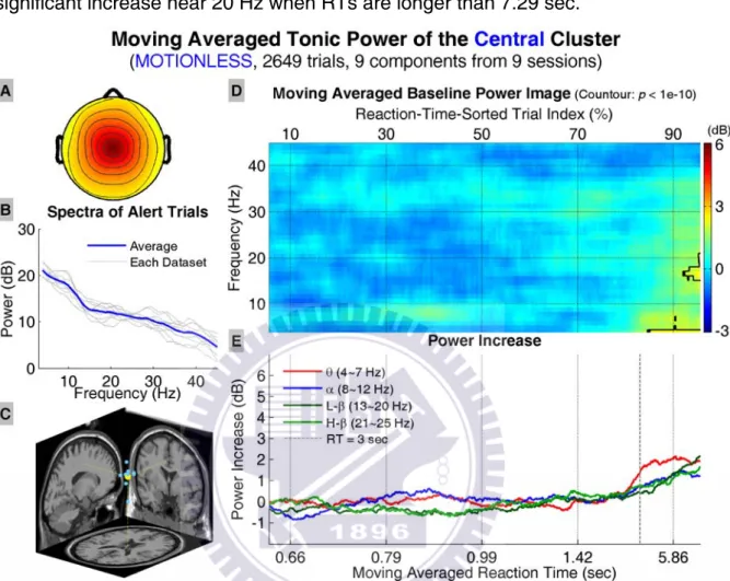
4.1.3.2 The Central and Parietal Clusters

Figure 14 shows the results of the central cluster, including the average scalp map, dipole source locations, baseline power spectra, tonic power image, and

(51)

trends of tonic power changes in four frequency bands. The power image and trends show significant increase in the low theta band when RTs are longer than 3 sec, and significant increase near 20 Hz when RTs are longer than 7.29 sec.

Figure 14: Results of the central cluster in the motionless datasets. All conventions follow Figure 13.

Figure 15 shows the results of the parietal cluster, including the average scalp map, dipole source locations, baseline power spectra, tonic power image, and trends of tonic power changes in four frequency bands. The power image and trends show the onset RTs of significant increase in the alpha and theta bands are around 2.27 sec and around 3 sec, respectively; in addition, such increase shifts to the lower frequencies when RTs further increase. Note that the power on the alpha band falls when RTs are longer than 3 sec, but theta band power continues to in-crease.

(52)

Figure 15: Results of the parietal cluster in the motionless datasets. All conventions follow Figure 13.

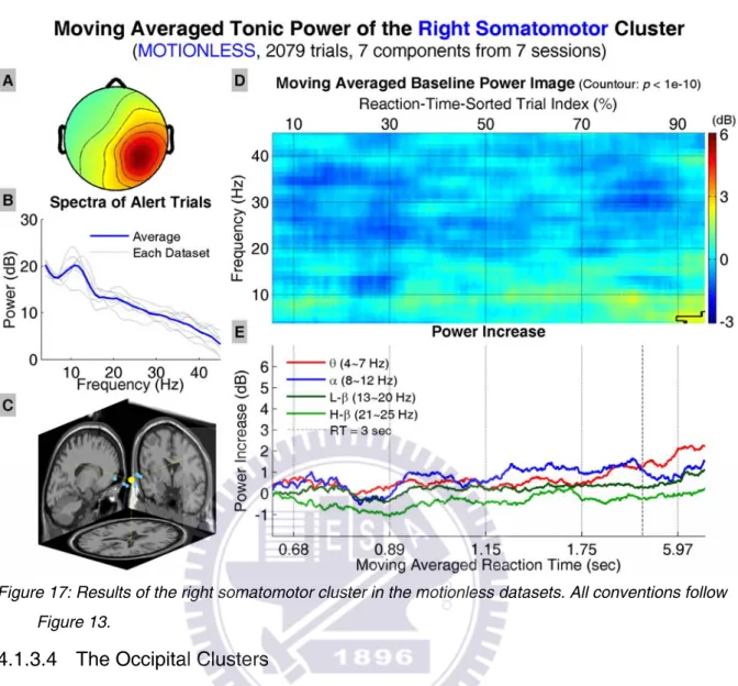
4.1.3.3 The Somatomotor Clusters

The results of the left and right somatomotor clusters, including the average scalp maps, dipole source locations, baseline power spectra, tonic power image, and trends of tonic power changes in four frequency bands, are shown in Figure 16 and Figure 17, respectively. The power images and trends show significant increase in the lower frequencies in the left (right) somatomotor cluster when RTs are longer than 2.17 (5.97) sec.

(53)

Figure 16: Results of the left somatomotor cluster in the motionless datasets. All conventions follow Figure 13.

(54)

Figure 17: Results of the right somatomotor cluster in the motionless datasets. All conventions follow Figure 13.

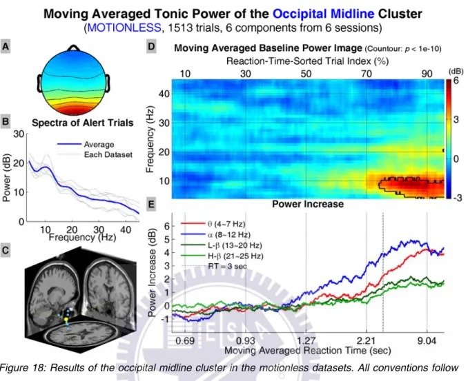
4.1.3.4 The Occipital Clusters

Figure 18 shows the results of the occipital midline cluster, including the aver-age scalp map, dipole source locations, baseline power spectra, tonic power imaver-age, and trends of tonic power changes in four frequency bands. The power image and trends start to show increase in the lower frequency bands when RTs are longer than ~1.27 sec. The power increase becomes significant when RTs are longer than ~3 sec, and shifts to the lower frequencies when RTs become even longer. The trend in alpha band power starts to decrease at RTs lower than those where the descending trend occurs in the theta band power.

(55)

Figure 18: Results of the occipital midline cluster in the motionless datasets. All conventions follow Figure 13.

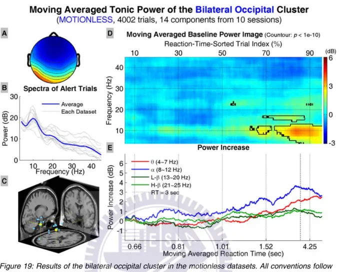
Figure 19 shows the results of the bilateral occipital cluster, including the av-erage scalp map, dipole source locations, baseline power spectra, tonic power im-age, and trends of tonic power changes in four frequency bands. The power image and trends start to show increase in the lower frequency bands when RTs are longer than ~1 sec. The power increase becomes significant when RTs are longer than ~1.3 sec and shifts to the lower frequencies when RTs become even longer. The trends in alpha band and low beta band power start to decrease when RTs are over ~3 sec; however, the trend in theta band power continues to increase as RTs further increase.

(56)

Figure 19: Results of the bilateral occipital cluster in the motionless datasets. All conventions follow Figure 13.

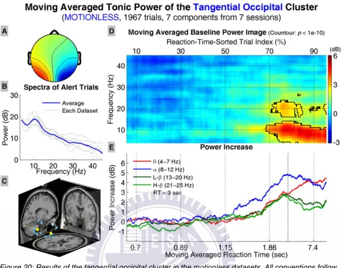
Figure 20 shows the results of the tangential occipital cluster, including the av-erage scalp map, dipole source locations, baseline power spectra, tonic power im-age, and trends of tonic power changes in four frequency bands. The power image and trends start to show increase in the lower frequency bands when RTs are longer than ~1.15 sec. The power increase becomes significant when RTs are longer than ~1.8 sec and shifts to the lower frequencies when RTs become even longer. The trends in alpha band and low/high beta band power start to decrease when RTs are over ~3 sec; however, the trend in theta band power continues to increase mono-tonically as RTs further increase.

(57)

Figure 20: Results of the tangential occipital cluster in the motionless datasets. All conventions follow Figure 13.

4.2 Motion Datasets

4.2.1 Behavioral Data

Table 2 shows the distribution of behavioral data of individual subjects in the “motion” condition. The shaded rows show the numbers of trials remained after EEG and behavioral artifact removal. Subjects are sorted in descending order by their drowsiness levels. In total, 52.84% of original trials in all subjects remained due to severe artifacts in the driving experiments. The car drifted to the left (right) in 51.7% (49.3%) of all the remained trials.

(58)

TABLE 2:BEHAVIORAL DATA OF MOTION DATASETS Trials Data Length (sec)* Trials Re-mained (%)** Max. RT (sec) Min. RT (sec) Avg. RT (sec) SD of RT (sec) Med. of RT (sec) Trials w. RT > 3 sec (%) Dev. to Left (%) 662 5815.36 -- 18.79 0.15 1.54 2.09 0.80 11.48 53.78 s44_070209 409 -- 61.78 14.74 0.45 1.74 2.25 0.84 14.18 52.57 683 6315.52 -- 11.3 0.02 1.29 1.54 0.87 6.88 53.44 s05_061019 319 -- 46.71 11.3 0.54 1.58 1.96 0.85 10.34 53.61 540 6515.16 -- 383.60 0.02 3.05 19.28 0.89 9.44 52.41 s35_070115 301 -- 55.74 27.40 0.33 1.56 2.87 0.80 6.98 55.48 685 6535.12 -- 22.52 0.02 1.53 1.89 1.14 4.67 51.39 s36_061122 330 -- 48.18 22.52 0.45 1.79 2.49 1.13 7.27 47.58 632 6562.20 -- 27.14 0.02 1.51 2.14 1.07 5.85 49.05 s40_070131 316 -- 50.00 27.14 0.38 1.59 2.54 1.07 5.06 46.52 711 6533.24 -- 12.74 0.10 1.01 1.21 0.70 2.25 51.62 s43_070202 315 -- 44.30 12.74 0.43 1.11 1.66 0.69 4.76 54.60 640 7061.04 -- 10.81 0.02 1.36 0.85 1.25 2.50 52.34 s31_061020 416 -- 65.00 8.39 0.52 1.39 0.68 1.29 2.16 51.68 4553 -- -- 383.6 0.02 1.57 6.84 0.97 6.04 52.01 All subjects 2406 -- 52.84 27.40 0.33 1.54 2.14 0.99 7.32 51.70

Note: shaded areas: distribution of the trials remained after artifacts removal. *: original datasets. **: datasets after artifacts removal.

Figure 21 shows the cumulative distribution of sorted reaction time across sub-jects in the “motion” datasets. The x- and y- axes are reaction time (in log scale) and percentage of RT-sorted index, respectively, and the vertical dashed line indicates 3-sec RT. The curve shows an approximate bi-linear distribution of RTs (when the x-axis is plotted in linear scale). About 10% of all remained trials have RTs longer than 3 sec, which suggest the subjects were not very drowsy in these trials.

(59)

Figure 21: Cumulative distribution curve of sorted reaction times in the motion datasets.

4.2.2 Clustered Scalp Maps and Dipole Locations

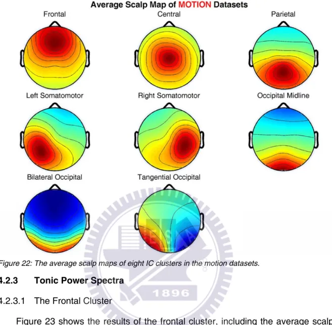
Eight clusters of independent components were identified based on their scalp maps from the results of ICA decomposition. The average scalp maps of these IC clusters are shown in Figure 22. Figure A25-Figure A48 show the scalp maps, and Table A11-Table A18 summarize the Talairach coordinates of each dipole in the remaining clusters.

(60)

Figure 22: The average scalp maps of eight IC clusters in the motion datasets.

4.2.3.1 The Frontal Cluster

Figure 23 shows the results of the frontal cluster, including the average scalp map, dipole source locations, baseline power spectra, tonic power image, and trends of tonic power changes in four frequency bands. The power image and trends in Figure 23 D and E, respectively, show increase in the theta band when the mean RTs are longer than 1.31 sec, and such increase shifts to the lower frequencies when RTs further increase and become significant (p < 10-10, corrected) when RTs are longer than 2.38 sec.

(61)

Figure 23: Results of the frontal cluster in the motion datasets. All conventions follow Figure 13.

4.2.3.2 The Central and Parietal Clusters

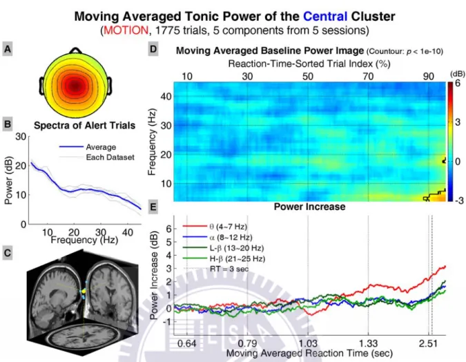
Figure 24 shows the results of the central cluster, including the average scalp map, dipole source locations, baseline power spectra, tonic power image, and trends of tonic power changes in four frequency bands. The power image and trends show significant increase in the low theta band when RTs are longer than ~2.5 sec, and significant increase near 20 Hz when RTs reach the maximum value.

(62)

Figure 24: Results of the central cluster in the motion datasets. All conventions follow Figure 13.

Figure 25 shows the results of the parietal cluster, including the average scalp map, dipole source locations, baseline power spectra, tonic power image, and trends of tonic power changes in four frequency bands. The power image and trends show increase in the alpha and beta bands when RTs increase moderately, and the increase shifts to the lower frequencies when RTs further increase. However, the increase in the entire power spectra does not reach the significance level.

(63)

Figure 25: Results of the parietal cluster in the motion datasets. All conventions follow Figure 13.

4.2.3.3 The Somatomotor Clusters

The results of the left and right somatomotor clusters, including the average scalp maps, dipole source locations, baseline power spectra, tonic power image, and trends of tonic power changes in four frequency bands, are shown in Figure 26 and Figure 27, respectively. Both somatomotor clusters show no significant changes when RTs increase.

(64)

Figure 26: Results of the left somatomotor cluster in the motion datasets. All conventions follow Figure 13.

(65)

Figure 27: Results of the right somatomotor cluster in the motion datasets. All conventions follow Figure 13.

4.2.3.4 The Occipital Clusters

Figure 28 shows the results of the occipital midline cluster, including the aver-age scalp map, dipole source locations, baseline power spectra, tonic power imaver-age, and trends of tonic power changes in four frequency bands. The power image and trends start to show increase in the lower frequency bands when RTs are longer than ~0.9 sec. The power increase in alpha (theta) band becomes significant when RTs are longer than ~1.6 (~2.4) sec, and the increase shifts to the lower frequencies when RTs become even longer. The increase in power in the alpha band is larger than that in the other bands, and it reaches a plateau when RTs are longer than ~1.23 sec; however, theta band power continues to increase monotonically with

(66)

Figure 28: Results of the occipital midline cluster in the motion datasets. All conventions follow Figure 13.

Figure 29 shows the results of the bilateral occipital cluster, including the av-erage scalp map, dipole source locations, baseline power spectra, tonic power im-age, and trends of tonic power changes in four frequency bands. The power image and trends start to show significant increase in the lower frequency bands (alpha and theta) when RTs are longer than ~0.9 sec, and shifts to the lower frequencies when RTs become even longer. The increase in alpha band power is higher than that in the other frequency bands. The trends in alpha band and beta band power start to decrease when RTs are over ~1.1 sec; however, the trend in theta band power continues to increase as RTs further increase.

(67)

Figure 29: Results of the bilateral occipital cluster in the motion datasets. All conventions follow Figure 13.

Figure 30 shows the results of the tangential occipital cluster, including the av-erage scalp map, dipole source locations, baseline power spectra, tonic power im-age, and trends of tonic power changes in four frequency bands. The power image and trends show increase in the alpha and beta bands when RTs increase, and the power increase in alpha (beta) band becomes significant when RTs are longer than 1.08 (0.99) sec, respectively. The trend in alpha (beta) band power reverses to the downside when RTs are longer than 1.23 (1.08) sec, and theta band power in-creases abruptly when RTs are longer than 1.61 sec.

(68)

Figure 30: Results of the tangential occipital cluster in the motion datasets. All conventions follow Figure 13.

4.3 Comparison Between Motionless and Motion Datasets

In real-life driving, the driver receives kinesthetic stimuli in addition to visual and auditory stimuli on the road. In order to investigate the effect of kinesthetic stimuli on the EEG data especially during drowsy driving, seven subjects who participated in both motion and motionless sessions were selected for comparison, and the be-havioral data and trends in EEG power spectra were compared between motion and motionless conditions. Subjects s01, s32, s41, and s42 did not participate in motion sessions, so their EEG data in the motionless datasets were not included in the comparison.

(69)

4.3.1 Behavioral data

Figure 31 shows the cumulative distributions of sorted reaction times across subjects in the “motion” (red trace) and “motionless” (blue trace) datasets, respec-tively. The x- and y- axes are reaction time (in log scale) and percentage of RT-sorted index, respectively, and the vertical dashed line indicates 3-sec RT. Both curves show approximate bi-linear distributions of RTs (when the x-axis is plotted in linear scale). The traces show that over 90% of trials have RTs less than 3 sec in the motion datasets, and only over 80% of trial RTs are below 3 sec in the motionless datasets. In addition, in the motion datasets, the shortest 1/3 (802 trials, RTs = 0.38~0.82 sec, mean = 0.66 ± 0.09 sec, median = 0.67 sec) and longest 1/3 (802 trials, RTs = 1.22~27.40 sec, mean = 2.97 ± 3.25 sec, median = 1.59 sec) RTs are longer than corresponding portions of RTs in the motionless datasets (shortest 1/3: 693 trials, RTs = 0.38~0.82 sec, mean = 0.71 ± 0.07 sec, median = 0.72 sec; long-est 1/3: 693 trials, RTs = 1.27~56.98 sec, mean = 6.15 ± 7.28 sec, median = 3.36 sec). The curves in both conditions are statistically different (p < 10-10_{, two-sample}

t-test); however, the middle 1/3 of RTs in both conditions are not significant

(mo-tionless datasets: 694 trials, RTs = 0.82~1.27 sec, mean = 1.00 ± 0.12 sec, median = 0.97 sec; motion datasets: 802 trials, RTs = 0.80~1.22 sec, mean = 0.99 ± 0.13 sec, median = 0.99 sec; p = 0.41).

虛擬駕駛環境下腦波頻譜與反應時間之關聯

國

立

交

通

大

學

電機與控制工程學系

碩 士 論 文

虛擬駕駛環境下腦波頻譜與反應時間之關聯

Changes in EEG Power Spectra Correlated with Driving

Performance in Simulated Driving Environment

研 究 生：陳青甫ˉˉˉ

指導教授：林進燈 教授

虛擬駕駛環境下腦波頻譜與反應時間之關聯

Changes in EEG Power Spectra Correlated with Driving

Performance in Simulated Driving Environment

研 究 生：陳青甫 Student: Ching-fu Chen

指導教授：林進燈 Advisor: Chin-Teng Lin

國 立 交 通 大 學

電 機 與 控 制 工 程 學 系

碩 士 論 文

虛擬駕駛環境下腦波頻譜與反應時間之關聯

摘 要

Changes in EEG Power Spectra Correlated with Driving

Performance in Simulated Driving Environment

ABSTRACT

誌 謝

Acknowledgements

Contents

Lists of Tables

Lists of Figures

Abbreviations

Chapter I Introduction

Chapter II Experiment Design and Setup

2.1 VR-Based Driving Simulator and Steward Motion Platform

2.2 Event-Related Lane-Departure Paradigm

2.3 Subjects

2.4 EEG Recording

Chapter III Data Analysis

3.1 Integration of EEG and Behavioral Data

3.2 Epoch Extraction

3.3 Artifact Removal

3.4 Independent Component Analysis (ICA)

[

]

[

]

( )

∏

( )

(

)

( )

[ ]

[

]

( )

( )

( )

(

)

3.5 Dipole Fitting

3.6 Computation of Tonic Power Spectra

3.7 Independent Component Clustering

Chapter IV Results

4.1 Motionless Datasets

4.2 Motion Datasets

4.3 Comparison Between Motionless and Motion Datasets

碩士論文

研究生：陳青甫ˉˉˉ

指導教授：林進燈教授

研究生：陳青甫 Student: Ching-fu Chen

國立交通大學

電機與控制工程學系

碩士論文

摘要

誌謝