國 立 交 通 大 學
應用數學系
數學建模與科學計算碩士班
碩
士
論
文
在 E 型代數結構下之 N 相黎曼空間的
單擺運動之確切理論與數值運算
The Exact Theory and Numerical Computations of
Pendulum Motions on Riemann Surface of
Genus N with Cut-Structure of Type E
研 究 生:王麗雲
指導教授:李榮耀 教授
在 E 型代數結構下之 N 相黎曼空間的
單擺運動之確切理論與數值運算
The Exact Theory and Numerical Computations of
Pendulum Motions on Riemann Surface of
Genus N with Cut-Structure of Type E
研 究 生:王麗雲 Student:Li-Yun Wang
指導教授:李榮耀 Advisor:Jong-Eao Lee
國 立 交 通 大 學
應用數學系數學建模與科學計算碩士班
碩 士 論 文
A ThesisSubmitted to Department of Applied Mathematics College of Science, Institute of Mathematical Modeling and Scientific Computing
National Chiao Tung University in Partial Fulfillment of the Requirements
for the Degree of Master
in
Applied Mathematics June 2013
Hsinchu, Taiwan, Republic of China
在 E 型代數結構下之 N 相黎曼空間的
單擺運動之確切理論與數值運算
研究生:王麗雲 指導教授:李榮耀 教授
國 立 交 通 大 學
應用數學系數學建模與科學計算碩士班
摘要
在此篇文章中,我們主要在探討理想的單擺運動。首先,藉由多項式去逼近,並探 討相對應之方程式,在這之中我們發現黎曼空間的理論是必要的,因此接著介紹如何造 出相對應的黎曼空間,並利用 Mathematica 幫助我們去計算相對應的黎曼空間上的路徑 積分及方程式上相關之性質。 再來,介紹橢圓函數的基本性質,我們利用橢圓函數解出原微分方程的實際解、週 期及相關性質。中 華 民 國 一 零 二 年 六 月
The Exact Theory and Numerical Computations of
Pendulum Motions on Riemann Surface of
Genus N with Cut-Structure of Type E
Student: Li-Yun Wang Advisor: Jong-Eao Lee
Institute of Mathematical Modeling and Scientific Computing
National Chiao Tung University
Abstract
In this paper, we study the ideal pendulum equation. First, we study the nonlinear
approximation of the exact theory, and the Riemann surface theory is needed. So we study the Riemann surface of genus N in various algebraic cut-structures. We then apply Mathematica to evaluate path integrals on those Riemann surfaces.
Secondly, we study the classical Elliptic functions. From which, we are able to solve the exact solution and certain properties of the pendulum motions.
誌 謝
這篇論文得以完成,首先要感謝我的指導教授-李榮耀老師,剛進研究所的 我根本不知道要做什麼,幸好有老師引導我進入狀況。老師不僅指導我們如何做 研究,更教導我們做學問的態度,受用無窮。 在研究所的這段期間,生活周遭發生了許多事情,謝謝研究室的朋友們:紫 琳、珮蓉、芷萱,妳們鼓勵我,給我正面的力量,讓我得以堅持下去;謝謝團隊 中的朋友們,尤其是名宏,不厭其煩地給我很多幫助;謝謝室友宜津,在碩論完 成的最後這兩個月,不僅一起努力,還給了我許多建議和幫忙;謝謝一起口試的 同伴們,有了大家的幫助減輕我許多負擔;謝謝好友紀葳,之後還得一起努力; 謝謝在教程認識的朋友們:懿方、宇清、濟駿以及佩萱姐,還好有你們的幫助讓 我在師培中心的修課能夠順利完成;謝謝在這三年中所有給過我幫助的朋友們以 及教授們,讓我得到許多經驗。 最後要感謝我的家人,在求學的路上,給我很大的支持和鼓勵,讓我能夠如 願地得到碩士學位,謝謝我的父母總是無怨無悔的付出,教導我許多人生大道理, 真的由衷地感謝,這份榮耀得歸於你們-我最親愛的父母。Contents
1 Introduction 1
2 Riemann Surface 4
2.1 Structures of the Riemann surfaces . . . 4
2.2 The contour in algebraic and geometric structure . . . 16
2.2.1 a- and b-cycles . . . 16
2.2.2 The equivalent path . . . 21
2.2.3 The integrals of 1 f (z) over a-, b-cycles . . . . 23
2.2.4 For horizontal cuts . . . 24
2.2.5 For vertical cuts . . . 25
2.2.6 For slant cuts . . . 28
2.2.7 Summary . . . 30
3 Nonlinear Approximations on Riemann Surfaces of the
4 Elliptic Functions 96
4.1 Basic concepts about the elliptic function . . . 96
4.1.1 Doubly-periodic function . . . 97
4.1.2 Period-parallelograms . . . 98
4.1.3 Simple properties of the elliptic function . . . 99
4.1.4 The order of an elliptic function . . . 100
4.2 Weierstrass elliptic function . . . 101
4.2.1 Periodicity and other properties of ℘(z) . . . 101
4.2.2 The differential equation satisfied by ℘(z) . . . 102
4.2.3 The integral formula for ℘(z) . . . 104
4.3 The theta function . . . 105
4.3.1 The four types of theta-function . . . 106
4.4 The Jacobian elliptic function . . . 112
5 The Exact Theory of the Pendulum Motion 116 5.1 Introduction of the simple pendulum motion . . . 116
5.2 The exact theory . . . 120
5.3 The periods . . . 125
5.5 Related knowledge . . . 131
6 Conclusion 132
Appendix 133
Chapter 1
Introduction
The simple pendulum is an idealized mathematical model of a pendulum. This is a bob on the end of a massless cord suspended from a pivot, with no friction in a closed system. As we give an initial push, it will swing at a constant amplitude back and forth.
In this paper, we consider a simple pendulum motion
u′′+ sin u = 0 . (1.0.1) Multiply the equation (1.0.1) by u′, then we have
u′u′′+ u′sin u = 0 . (1.0.2) Integrate the equation (1.0.2) and compute it, we can get
1 2(u
′)2− cos u = E , where E is the integration constant. ⇒ (u′)2 = 2(E + cos u) ⇒ u′ =±√2(E + cos u) ⇒ du dt =± √ 2(E + cos u) (1.0.3)
The equation (1.0.3) can then be expressed as ∫ 1 √ 2(E + cos u) du =± ∫ dt . (1.0.4)
Indeed the equation (1.0.4) is not easy to solve.
At first, we can analyze the properties of the solution of the equation. We know that sin u can be expanded by Taylor series
sin u = ∞ ∑ k=0 (−1)k (2k + 1)!u 2k+1
, for all values of u.
Use the nonlinear approximation we can get
sin u≈ N ∑ k=0 (−1)k (2k + 1)!u
2k+1, for all positive integer values of N .
Let P2N +1(u) = N ∑ k=0 (−1)k (2k + 1)!u 2k+1
So the equation(1.0.1) becomes to
u′′+ P2N +1(u) = 0 .
As above, after computing we obtain the following integral equation ∫ 1 √ 2(E− P2N +2(u)) du =± ∫
dt , where E is the integration constant.
Since 2(E− P2N +2(u)) is a polynomial of u, it can be written as 2(E− P2N +2(u)) = (u− u1)(u− u2)· · · (u − u2N +2)
= 2N +2∏
k=1
(u− uk) ,
where uk’s are the roots of the equation 2(E− P2N +2(u)) = 0 . Thus, the function theory of solutions u of the equation involves
v u u t2N +2∏ k=1 (u− uk).
Consider a function f (z) = v u u t∏n k=1
(z− zk) and it is not single-valued on the
complex planeC that we will have more to say about later. We use algebra and analysis to develop a new surface such that f becomes a single-valued function on it. This surface is called a Riemann Surface.
But later, in order to get the exact solution of the original equation, we use the elliptic functions, which Chapter 4 and Chapter 5 will discuss it in detail.[4]
Chapter 2
Riemann Surface
2.1
Structures of the Riemann surfaces
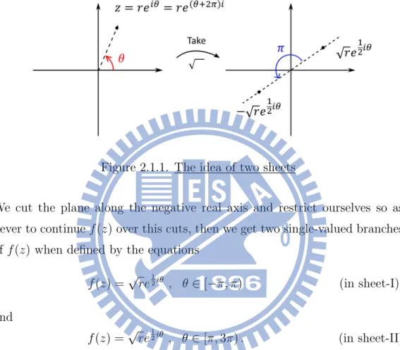
In this section, we use the function f (z) =√z to show how to construct the corresponding Riemann surface for f (z) . Using polar form, let
z = rei(θ+2kπ), r̸= 0 , k ∈ Z . Then we have f (z) =√re12i(θ+2kπ) =√re12iθekπi = { √ re12iθ if k is even −√re12iθ if k is odd
which is a two-valued function since it has different values as θ increases by 2π. Here we want to make f (z) single-valued, so we modify its domainC to build the corresponding Riemann surface such that f becomes single-valued on it.
Beginning with z = reiθ, r ̸= 0 , we have f(z) = √z = √re12iθ. Holding
r constant, and going along any closed path once around the origin so that θ increases by 2π, f (z) changes to √re12i(θ+2π) =−√re
1
negative of its original value. (Show in Figure 2.1.1.)
Continuing above way then θ increases by 2π and f (z) returns to the original value.
Figure 2.1.1. The idea of two sheets
We cut the plane along the negative real axis and restrict ourselves so as never to continue f (z) over this cuts, then we get two single-valued branches of f (z) when defined by the equations
f (z) =√re12iθ , θ∈ [−π, π) (in sheet-I)
and
f (z) =√re12iθ , θ∈ [π, 3π) . (in sheet-II)
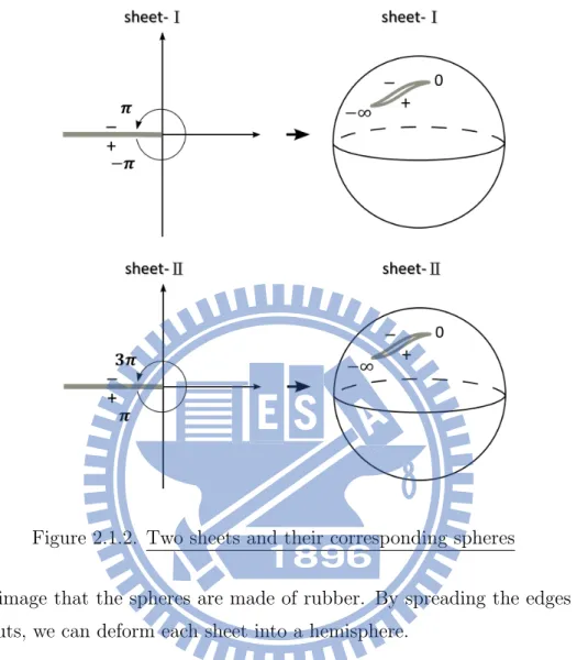
The cut on each sheet has two edges. We label the starting edge with “+” and the terminal edge with “−”. (Show in Figure 2.1.2.) Imagine that the surface as two sheets lying over the complex plane, each cut along the negative real axis.
Moreover, we extend the complex plane with the “point” at infinity to consti-tute the extended complex plane. Use stereographic projection, we can think of the two sheets as spheres.
Figure 2.1.2. Two sheets and their corresponding spheres
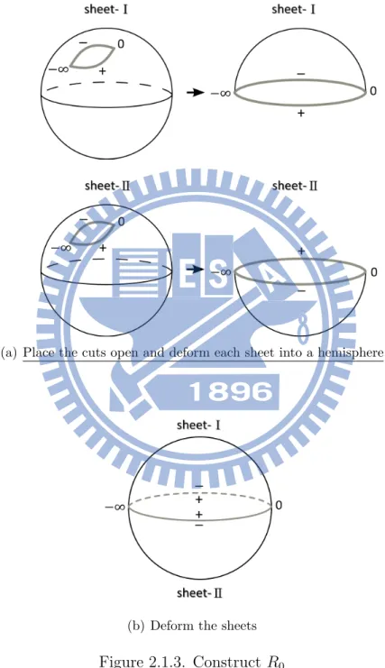
Now image that the spheres are made of rubber. By spreading the edges of the cuts, we can deform each sheet into a hemisphere.
Paste the hemispheres each other together (+)edge of sheet-I with (−)edge of sheet-II and (−)edge of sheet-I with (+)edge of sheet-II. Then we can derive a sphere, which is called the Riemann surface of genus 0 , denoted by R0. (Show in Figure 2.1.3.)
Hence, (+)edge of sheet-I is equivalent to (−)edge of sheet-II and (−)edge of sheet-I is equivalent to (+)edge of sheet-II in the Riemann surface. As we cross the cut, we move around the other sheet.
(a) Place the cuts open and deform each sheet into a hemisphere
(b) Deform the sheets
The following are two examples, we will construct whose corresponding Rie-mann surface in a similar way.
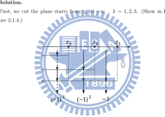
Example 2.1.
Construct the Riemann surface for f (z) = v u u t∏3 k=1 (z− zk) = 3 ∏ k=1 √ z− zk, zk ∈ R and z1 > z2 > z3. Solution.
First, we cut the plane starts from zk to −∞ , k = 1, 2, 3. (Show in
Fig-ure 2.1.4.)
Figure 2.1.4. The cut from zk to −∞
Crossing one cut, we move around the other sheet, the argument of z in-creases by 2π then the argument of f (z) inin-creases by π which is just the negative of its original value. As we cross one cut, we need to change the sign by “−1”. We find that crossing odd times will change the sign and even times will keep its same value. So there are branch cuts along [−∞, z3] and [z2, z1] as illustrated in the in Figure 2.1.5.
Figure 2.1.5. The cut structure
Second, placing the cuts open, pasting two sheets together (+)edge with (−)edge, and using the same idea as above. Then we obtain the corre-sponding Riemann surface of genus 1 for f (z), denoted by R1. (Show in Figure 2.1.6.)
(a) Cuts on the two spheres
(b) Deform the two sheets
(c) Construct R1
Example 2.2.
Construct the Riemann surface for f (z) = v u u t∏4 k=1 (z− zk) = 4 ∏ k=1 √ z− zk, zk∈ R and z1 > z2 > z3 > z4. Solution.
As in Example 2.1, we cut the plane start from zk to −∞ , k = 1, . . . , 4.
(Show in Figure 2.1.7.)
Figure 2.1.7. The cut from zk to −∞
Then there are branch cuts along [z4, z3] and [z2, z1]. (Show in Figure 2.1.8.)
Figure 2.1.9. Construct cuts on two spheres
Figure 2.1.10. The deformation from the Figure 2.1.9.
Paste two sheets together (+)edge with (−)edge, then we obtain the corre-sponding Riemann surface of genus 1 for f (z), denoted by R1.
We found f (z) of 3 or 4 roots have different algebraic structures but same geometric graph with 1 holes. That is no matter 3 or 4 points, we can construct corresponding Riemann surface of genus 1.
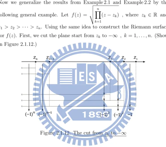
Now we generalize the results from Example 2.1 and Example 2.2 by the
following general example. Let f (z) = v u u t∏n k=1 (z− zk) , where zk ∈ R and
z1 > z2 > · · · > zn. Using the same idea to construct the Riemann surface
for f (z). First, we cut the plane start from zk to−∞ , k = 1, . . . , n. (Show
in Figure 2.1.12.)
Figure 2.1.12. The cut from zk to −∞
Then we discuss the cuts structure in two cases according to n is odd or even.
Case i. If n∈ odd, denoted by 2N − 1.
There are cuts along [−∞, z2N−1], [z2N−2, z2N−3],· · · , [z2j, z2j−1],· · · , [z4, z3], [z2, z1] .
Figure 2.1.14. Together two sheets
Then we obtain the corresponding Riemann surface of genus N− 1 for f (z), denoted by RN−1. (Show in Figure 2.1.15.)
Figure 2.1.15. Geometric graph of RN−1
Case ii. If n∈ even, denoted by 2N.
There are cuts along [z2N, z2N−1], [z2N−2, z2N−3],· · · , [z2j, z2j−1],· · · , [z4, z3], [z2, z1]
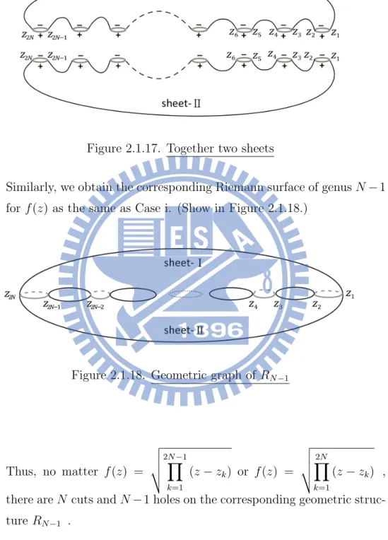
Figure 2.1.17. Together two sheets
Similarly, we obtain the corresponding Riemann surface of genus N−1 for f (z) as the same as Case i. (Show in Figure 2.1.18.)
Figure 2.1.18. Geometric graph of RN−1
Thus, no matter f (z) = v u u t2N∏−1 k=1 (z− zk) or f (z) = v u u t∏2N k=1 (z− zk) ,
there are N cuts and N−1 holes on the corresponding geometric struc-ture RN−1 .
2.2
The contour in algebraic and geometric
structure
We already comprehend the relation of algebraic and geometric structure
for f (z) = v u u t∏n k=1
(z− zk) and how to construct the corresponding Riemann
surface. In this section, we will show that the contour on the algebraic structure and its corresponding geometric structure.
Note that
1. In the algebraic structure, solid line means the contour in sheet-I and dash line means the contour in sheet-II.
2. In the geometric structure, solid line means the contour in overhead Riemann surface and dash line means the contour in ventral Riemann surface.
2.2.1
a- and b-cycles
Every closed curve on Riemann surface can be deformed into an integral combination of the loop-cut ai and bi, i = 1, 2, ..., N . So in this section, we
will introduce a-,b-cycles, which can help us simplifying the computation.
• a-cycle is a simple closed curve enclosing a finite cut (the endpoint of cut is a finite number).
• b-cycle is a simple closed curve starting from (+)edge of a cut (it maybe finite cut or infinite cut) without enclosed by any a-cycle, to (+)edge of another cut enclosed by a a-cycle. Then the curve crosses through (−)edge of this cut and goes into sheet-II, and finally arrives to the (−)edge of the starting cut.
Each a-cycles are non-overlapping and each b-cycles are non-overlapping. Note that a- and b-cycles have the same amount.
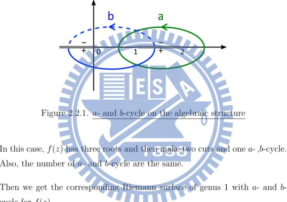
Here we take f (z) =√z(z− 1)(z − 2) for example to illustrate a- ,b-cycles on the cut plane and on the Riemann surface.
The a- and b-cycle are shown in Figure 2.2.1 and Figure 2.2.2.
Figure 2.2.1. a- and b-cycle on the algebraic structure
In this case, f (z) has three roots and then make two cuts and one a- ,b-cycle. Also, the number of a- and b-cycle are the same.
Then we get the corresponding Riemann surface of genus 1 with a- and b-cycle for f (z).
(a) a- ,b-cycle on two sheets
(b) R1 for f (z) with a- ,b-cycle
Figure 2.2.2. a- and b-cycle on the corresponding geometric structure
Here we review some famous theorems.
Theorem 2.1. (Cauchy-Goursat Theorem)
If a function f is analytic at all points interior to and on a simple closed contour C, then ∫
C
Theorem 2.2. (Cauchy Theorem)
Let C and C1, C2, . . . , Cn denote counterclockwise simple closed contours.
Let all the contours Ci’s be outside each other but inside C. If a function f
is analytic in the closed and “holey” region consisting of those contours and all points between them, then
∫ C f (z)dz = n ∑ i=1 ∫ Ci f (z)dz . Corollary 2.1.
Let C1 and C2 denote counterclockwise simple closed contours, where C2 is interior to C1. If a function f is analytic in the closed and “holey” region consisting of those contours and all points between them, then
∫ C1 f (z)dz = ∫ C2 f (z)dz .
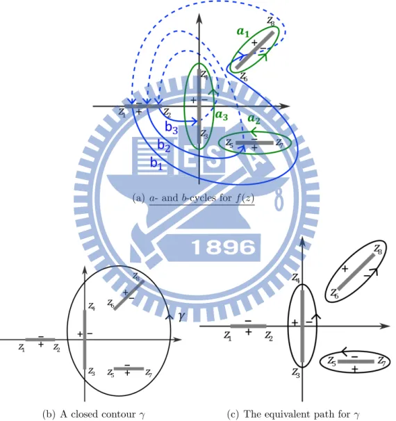
Take another example, let f (z) = v u u t∏8 k=1
(z− zk) , and make ai and bi cycles,
i = 1, 2, 3. Consider a closed contour γ as shown in Figure 2.2.3.
(a) a- and b-cycles for f (z)
(b) A closed contour γ (c) The equivalent path for γ
Figure 2.2.3. Deform γ into a combination of a-cycles
Using Cauchy Theorem, then γ can be deformed into a combination of ai
Any closed curve on the Riemann surface can be deformed into a combination of a- and b-cycles. Thus, in this paper, we will consider the integrals of f (z) over a- and b-cycles that help us to evaluate the integrals easier.
2.2.2
The equivalent path
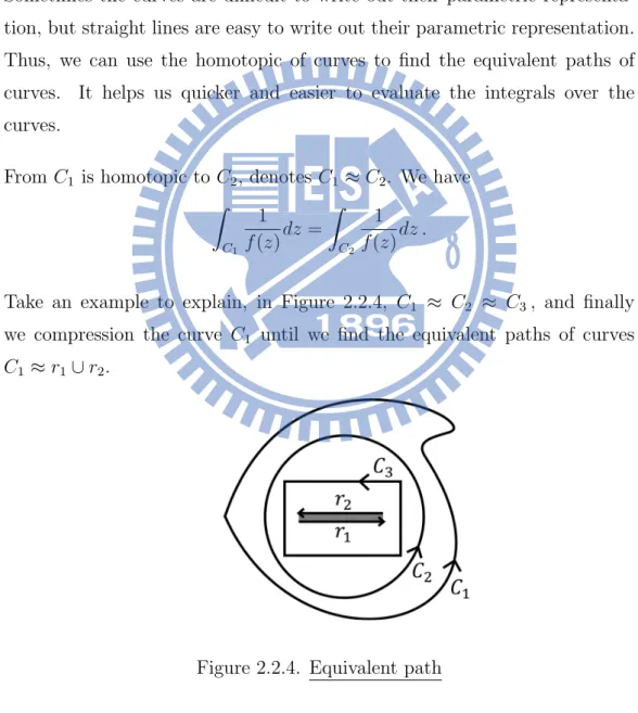
Sometimes the curves are difficult to write out their parametric representa-tion, but straight lines are easy to write out their parametric representation. Thus, we can use the homotopic of curves to find the equivalent paths of curves. It helps us quicker and easier to evaluate the integrals over the curves.
From C1 is homotopic to C2, denotes C1 ≈ C2. We have ∫ C1 1 f (z)dz = ∫ C2 1 f (z)dz .
Take an example to explain, in Figure 2.2.4, C1 ≈ C2 ≈ C3, and finally we compression the curve C1 until we find the equivalent paths of curves C1 ≈ r1∪ r2.
Therefore we obtain ∫ C1 1 f (z)dz = ∫ C2 1 f (z)dz = ∫ C3 1 f (z)dz = ∫ r1∪r2 1 f (z)dz = ∫ r1 1 f (z)dz + ∫ r2 1 f (z)dz .
Hence we can replace the complicated path C1 for simple path r1 ∪
r2.
We take f (z) =√z(z− 1)(z − 2) for example to show the equivalent path.
(a) a, b-cycle
(b) The equivalent path for a, b-cycle
2.2.3
The integrals of
1
f (z)
over a-, b-cycles
As in Section2.1, we consider the function f (z) =√z . Let θ2 = θ1+ 2π and z1 = reiθ1 and z2 = reiθ2, r ̸= 0 , where θ1 denotes the argument in sheet-I and θ2 denotes the argument in sheet-II. Then on the complex plane z1 = z2, but f (z2) = √ z2 = √ re12iθ2 =√re 1 2i(θ1+2π) =√re12iθ1eiπ=−√re 1 2iθ1 =−√z1 =−f(z1). Figure 2.2.5. f (z1)̸= f(z2)
That is because the difference of argument between z in sheet-I and sheet-II is 2π, that is the difference between f (z)|(I) and f (z)|(II) is π. Hence, we have
f (z)|(I) =−f(z)|(II)
where f (z)|(I) denotes the computation of f (z) in sheet-I and f (z)|(II) de-notes the computation of f (z) in sheet-II.
2.2.4
For horizontal cuts
• The problem as using Mathematica
We want to calculate ∫ 1 f (z)dz , where f (z) = v u u t∏n k=1 (z− zk) , by using
Mathematica we can obtain the value. But when we compute the integrals by Mathematica, we found something uncommon.
We observe that the computation of f (z) in sheet-I is not equivalent to the computation of f (z) in Mathematica as the argument is−π. Take √−1 for example, in sheet-I the argument of −1 is −π and the argument of √−1 is −π
2, then we have √
−1 = e−π
2i =−i . But using Mathematica we obtain
√
−1 M ath.
= i , which we must multiply by −1 to get the correct value. The reason is in Mathematica the argument belongs to (−π, π] which is different from in sheet-I the argument belongs to [−π, π).
Figure 2.2.6. The value of√−1 in Mathematica and in theory
• Modification
For convenience, we denote f (z)M ath.= −f(z) , which signifies that the polyno-mial f (z) in front of “M ath.= ” is the value of f (z) in theory and the polynomial f (z) behind the “M ath.= ” is the value of f (z) in Mathematica.
Compare the value of f (z) with z in sheet-I and in Mathematica. We then observed that sometimes the computation of Mathematica needed to modify, collating as following.
Lemma 2.1. If
n
∏
k=1
(z − zk) = reiθ in sheet-I with horizontal cut,
then
f (z)|(I) = {
f (z)|M ath. θ ∈ (−π, π)
−f(z)|M ath. θ =−π
where f (z)|M ath. denotes the computation of f (z) in Mathematica.
Proof.
Since −π does not in (−π, π], Mathematica will transform re−iπ into reiπ, but f (re−iπ) and f (reiπ) are different.
In theory: − 1 = e−iπ ⇒√−1 = e−iπ2 =−i
In Mathematica: − 1 = e−iπ Math.= eiπ ⇒√−1 = eiπ2 = i
So f (z)M ath.= −f(z) if θ = −π in Mathematica.
2.2.5
For vertical cuts
• The problem as using Mathematica
We cut the plane along the positive imaginary axis and define tha
z− zk = reiθ , θ∈ [− 3 2π, 1 2π) (in sheet-I) and z− zk = reiθ , θ∈ [ 1 2π, 5 2π) . (in sheet-II)
The cut on each sheet has two edges. We label the starting edge with “+” and the terminal edge with “−” .
Suppose that f (z) =√z , z = ri .
In sheet-I, z =|z|eiθ, θ ∈ [−3 2π, 1 2π) then √ z =|z|12ei θ 2 ,θ 2 ∈ [− 3 4π, 1 4π)
In sheet-II, z = |z|eiθ, θ ∈ [1 2π, 5 2π) then √ z =|z|12ei θ 2 ,θ 2 ∈ [ 1 4π, 5 4π)
Figure 2.2.7. The domain and image on two sheets for vertical cut
• Modification
Compare the difference between the computation in theory and in Mathe-matica as illustrated in the in Figure 2.2.8.
Figure 2.2.8. The difference between in theory and in Mathematica for vertical cut
So we need to modify the computation in Mathematica, collating as following.
Lemma 2.2. If z in sheet-I for vertical cut, then √ z− zk M ath. = −√z− zk arg(z− zk)∈ [− 3 2π,−π] √ z− zk arg(z− zk)∈ (−π, 1 2π)
where arg(z − zk) denotes the argument of f (z).
Proof.
Let z in sheet-I and using polar form z− zk = reiθ. When θ ∈ (−π,
π 2), the argument in theory or Mathematica is the same. When θ ∈ [−3π
2 ,−π], Mathematica will conversion θ into θ + 2π where θ + 2π∈ [π
2, π] and re iθ = re(θ+2π)i, but In theory: √z− zk = √ reθ2i In Mathematica: √z− zk = √ reθ+2π2 i =−√re θ 2i Thus, if θ∈ [−3π 2 ,−π] , √ z− zk M ath. = −√z− zk.
2.2.6
For slant cuts
• The problem as using Mathematica
We cut the plane along a straight line which slope is m = tan α , 0 < α≤ π . Notice that the cut with α means the slope of the straight line where the cut on is m = tan α , 0 < α≤ π . We define that
z = reiθ , θ∈ [α − 2π, α) (in sheet-I) and
z = reiθ , θ ∈ [α, α + 2π) . (in sheet-II) The cut on each sheet has two edges. We label the starting edge with “+” and the terminal edge with “−” .
Suppose that f (z) =√z , z ∈ C .
In sheet-I, z =|z|eiθ, θ ∈ [α−2π, α) then√z =|z|12ei
θ 2 ,θ 2 ∈ [ α− 2π 2 , α 2)
In sheet-II, z =|z|eiθ, θ ∈ [α, α+2π) then√z =|z|12ei
θ 2 ,θ 2 ∈ [ α 2, α + 2π 2 ) • Modification
Compare the difference between the computation in theory and in Mathe-matica as illustrated in the Figure 2.2.10.
Figure 2.2.9. The domain and image on two sheets for the cut with α
Lemma 2.3. If the cut with zk on the line where the slope of line is
m = tan α , 0 < α ≤ π . and z in sheet-I, then √ z− zk M ath. = { −√z− zk arg(z− zk)∈ [α − 2π, −π] √ z− zk arg(z− zk)∈ (−π, α) Proof.
Let z in sheet-I and using polar form z− zk = reiθ where arg(z− zk) = θ .
When θ∈ (−π, α), the argument in theory and in Mathematica is the same. When θ ∈ [α − 2π, −π], Mathematica will transform θ into θ + 2π where θ + 2π∈ [α, π] and reiθ = re(θ+2π)i, but
In theory: √z− zk = √ reθ2i In Mathematica: √z− zk = √ reθ+2π2 i =−√re θ 2i So if θ∈ [α − 2π, −π], √ z− zk M ath. = −√z− zk.
2.2.7
Summary
Because sometimes the form of integration is complex, if we could simplify the way about modify the sign of f (z), it will help us to get right value easier. We divided domain C into many blocks to discuss way to modify on slant cuts. It can help us reduce the steps of modifying f (z).
Definition 2.1. Any slant cut whose slope of line is m = tan α , 0 < α≤ π and the end points of cut are zk = xk+ iyk and zk+1 = xk+1+ iyk+1. Define
the domain L as
L = (x, y) : y− yk > tan α (x− xk) when tan α > 0
Lemma 2.4. If f (z) = √z− zk
√
z− zk+1 for the cut with α. We
divided domain C into 6 areas as illustrated in the Figure 2.2.11. (B1) ={ (x, y) | (x, y) ∈ L and y ≥ yk+1} (B2) ={ (x, y) | (x, y) ∈ L and yk ≤ y < yk+1} (B3) ={ (x, y) | (x, y) ∈ L and y < yk} (M ) = (B4) ∪ (B5) ∪ (B6) = { (x, y) | (x, y) ∈ C \ L } ∪ { (x, y)| y− yk x− xk = tan α } then we have f (z) M ath.= { −f(z) if z ∈ (B2) ∪
{ the cut with (+)edge of sheet-I } f (z) otherwise.
Proof.
Figure 2.2.11. Divided domain C into 6 blocks
(1) z ∈ (B1) : arg(z− zk), arg(z − zk+1)∈ [α − 2π, −π] √ z− zk M ath. = −√z− zk and √ z− zk+1 M ath. = −√z− zk+1 f (z) M ath.= f (z) (2) z ∈ (B2) : arg(z− zk)∈ [α − 2π, −π] then √ z− zk M ath. = −√z− zk
√ z− zk+1 ∈ [−π, π] then √ z− zk+1 M ath. = √z− zk+1 f (z) M ath.= −f(z) (3) z ∈ (B3) ∪ (M ) : arg(z− zk), arg(z− zk+1)∈ [−π, π] √ z− zk M ath. = √z− zk and √ z− zk+1 M ath. = √z− zk+1 f (z) M ath.= f (z)
(4) z ∈the cut with (+)edge of sheet-I: arg(z− zk) = α− 2π then √ z− zk M ath. = −√z− zk arg(z− zk+1) = α− π then √ z− zk+1 M ath. = √z− zk+1 f (z) M ath.= −f(z)
(5) z ∈the cut with (−)edge of sheet-I: arg(z− zk) = α then √ z− zk M ath. = √z− zk arg(z− zk+1) = α− π then √ z− zk+1 M ath. = √z− zk+1 f (z) M ath.= f (z)
There are two examples we calculate the integrals in theory and in Mathemat-ica respectively, and also draw the path on the the corresponding Riemann surface.
Example 2.3. Evaluate ∫
1
f (z)dz over a3, b1 and b2 cycles, where
f (z) =√(z + 2 + i)(z + 2− i)(z + 1 + i)(z + 1 − i)(z − 0)(z − 1)(z − 1 − i)(z − 1 − 2i) . Let z1 =−2 − i, z2 =−2 + i, z3 =−1 − i, z4 =−1 + i, z5 = 0, z6 = 1, z7 =
(a) The cut plane
(c) The regions need changing sign of cuts
Using region of modify to get result by Mathematica: The region needs changing sign of √z− z1
√
z− z3 is { (+)edge of the cut z1z3 }. The region needs changing sign of
√ z− z2
√
z− z4 is { (+)edge of the cut z2z4 }. The region needs changing sign of
√ z− z5
√
z− z6 is { z = x + iy| x < 0 , 0 ≤ y < 1 }∪ { (+) edge of the cut z2z4 }. The region needs changing sign of √z− z7
√
z− z8 is { z = x + iy | x < 1 , 1 ≤ y < 2 }. We let region of modify (M ) = { z = x + iy | x < 0 , 0 ≤ y < 1 } ∪ { z = x + iy| x < 1 , 1 ≤ y < 2 } ∪ { (+)edge of the cut z1z3 } \ { (+)edge of the cut z2z4 }. 1. Evaluate ∫ a3 1 f (z)dz
Figure 2.2.12. The contour a3 in the cut plane
a3 : Consider the equivalent path a∗3 = a∗31 ∪
a∗32, where
a∗31= the path on the horizontal cut from−2 − i to −1 − i on (+)edge of sheet-I and
a∗32= the path on the horizontal cut from −1 − i to −2 − i on (−)edge of sheet-I.
Figure 2.2.13. The equivalent path for a3
(1) a∗31 : Let z = r− i , r : −2 → −1 , dz = dr and z ∈ (M) then f (z)M ath.= −f(z) ∫ a∗31 1 f (z)dz M ath. = − ∫ −1 −2 1 f (r− i)dr
(2) a∗32 : Let z = r− i , r : −1 → −2 , dz = dr and z /∈ (M) then f (z)M ath.= f (z) ∫ a∗32 1 f (z)dz M ath. = ∫ −2 −1 1 f (r− i)dr
By (1),(2) and Cauchy Theorem we can obtain ∫
a3
1
f (z)dz , which value is shown in the Appendix A.0.1.
2. Evaluate ∫
b1
1 f (z)dz
b1 : Consider the equivalent path
b∗1 = b∗11∪b∗12∪a∗31∪b∗13∪b∗14∪b∗15∪b∗16∪b∗17∪b∗18∪b∗19∪b∗201 ∪
(a) The contour b3 in the cut plane
b∗11 = the path on the vertical line from −2 + i to −2 on sheet-I, b∗12 = the path on the vertical line from −2 to −2 − i on sheet-I, b∗13 = the path on the vertical line from −1 − i to −1 on sheet-I, b∗14 = the path on the horizontal line from −1 to 0 on sheet-I, b∗15 = the path on the vertical cut from 0 to i on (−)edge of sheet-I, b∗16 = the path on the horizontal line from i to 1 + i on sheet-I,
b∗17 = the path on the vertical cut from 1 + i to 1 + 2i on (−)edge of sheet-II,
b∗18 = the path on the vertical cut from 1 + 2i to 1 + i on (+)edge of sheet-II,
b∗19 = the path on the horizontal line from 1 + i to i on sheet-II, b∗201 = the path on the horizontal line from i to −1 + i on sheet-II, and b∗202 = the path on the horizontal line from−1 + i to −2 + i on (−)edge of sheet-II.
(1) b∗11 : Let z = −2 + ri , r : 1 → 0 , dz = idr and z ∈ (M) then f (z)M ath.= −f(z) ∫ b∗11 1 f (z)dz M ath. = − ∫ 0 1 i f (−2 + ri)dr
(2) b∗12 : Let z = −2 + ri , r : 0 → −1 , dz = idr and z /∈ (M) then f (z)M ath.= f (z) ∫ b∗12 1 f (z)dz M ath. = ∫ −1 0 i f (−2 + ri)dr
(3) b∗13 : Let z = −1 + ri , r : −1 → 0 , dz = idr and z /∈ (M) then f (z)M ath.= f (z) ∫ b∗13 1 f (z)dz M ath. = ∫ 0 −1 i f (−1 + ri)dr
(4) b∗14: Let z = r , r :−1 → 0 , dz = dr and z ∈ (M) then f(z)M ath.=
−f(z) ∫ b∗14 1 f (z)dz M ath. = − ∫ 0 −1 1 f (r)dr
(5) b∗15: Let z = ri , r : 0 → 1 , dz = idr and z /∈ (M) then f(z)M ath.= f (z) ∫ b∗15 1 f (z)dz M ath. = ∫ 1 0 i f (ri)dr
(6) b∗16 : Let z = r + i , r : 0 → 1 , dz = dr and z ∈ (M) then f (z)M ath.= −f(z) ∫ b∗16 1 f (z)dz M ath. = − ∫ 1 0 1 f (r + i)dr
(7) b∗17≡ the path on the vertical cut from 1 + i to 1 + 2i on (+)edge of sheet-I,
so z ∈ (M). Let z = 1 + ri , r : 1 → 2 and dz = idr then f (z)M ath.= −f(z) ∫ b∗17 1 f (z)dz = ∫ 1+i99K1+2i− 1 f (z)dz = ∫ 1+i→1+2i+ 1 f (z)dz M ath. = − ∫ 2 1 i f (1 + ri)dr (8) b∗18≡ the path on the vertical cut from 1 + 2i to 1 + i on (−)edge
of sheet-I,
so z /∈ (M). Let z = 1 + ri , r : 2 → 1 and dz = idr then f (z)M ath.= f (z) ∫ b∗18 1 f (z)dz = ∫ 1+2i99K1+i+ 1 f (z)dz = ∫ 1+2i→1+i− 1 f (z)dz M ath. = ∫ 1 2 i f (1 + ri)dr (9) b∗19 : Let z = r + i , r : 1 → 0 , dz = dr and z ∈ (M) then
f (z)M ath.= −f(z) ∫ b∗39 1 f (z)dz = ∫ iL991+i 1 f (z)dz =− ∫ i←1+i 1 f (z)dz M ath. = ∫ 0 1 1 f (r + i)dr (10) b∗201 : Let z = r + i , r : 0 → −1 , dz = dr and z ∈ (M) then
f (z)M ath.= −f(z) ∫ b∗201 1 f (z)dz = ∫ −1+iL99i 1 f (z)dz =− ∫ −1+i←i 1 f (z)dz M ath. = ∫ −1 0 1 f (r + i)dr
(11) b∗202 ≡ the path on the horizontal cut from −1 + i to −2 + i on (+)edge of sheet-I.
Let z = r +i , r :−1 → −2 , dz = dr and z /∈ (M) then f(z) M ath.= f (z) ∫ b∗202 1 f (z)dz = ∫ −2+iL99 −1+i− 1 f (z)dz = ∫ −2+i+ ←−1+i 1 f (z)dz M ath. = ∫ −2 −1 1 f (r + i)dr
By (1)∼(11) and Cauchy Theorem we can obtain ∫
b1
1
f (z)dz , which value is shown in the Appendix A.0.2.
3. Evaluate ∫
b2
1 f (z)dz
Figure 2.2.14. The contour b2 in the cut plane
b2 : Consider the equivalent path
b∗21 = the path on the vertical line from 0 to i on sheet-II,
b∗22 = the path on the horizontal line from i to −1 + i on sheet-II.
Figure 2.2.15. The equivalent path for b2
(1) b∗21≡ the path on the vertical cut from 0 to i on (+)edge of sheet-I,
so z ∈ (M). Let z = ri , r : 0 → 1 and dz = idr then f(z)M ath.= −f(z) ∫ b∗21 1 f (z)dz = ∫ 099Ki− 1 f (z)dz = ∫ 0→i+ 1 f (z)dz M ath. = − ∫ 1 0 i f (ri)dr (2) b∗22 : Let z = r + i , r : 0 → −1 , dz = dr and z ∈ (M) then
f (z)M ath.= −f(z) ∫ b∗32 1 f (z)dz = ∫ 1+iL99i 1 f (z)dz =− ∫ 1+i←i 1 f (z)dz M ath. = ∫ −1 0 1 f (r + i)dr
By (1),(2) and Cauchy Theorem we can obtain ∫
b2
1
f (z)dz , which value is shown in the Appendix A.0.3.
Example 2.4. Evaluate ∫
1
f (z)dz over a3, b1 and b2 cycles, where
f (z) =√(z + 2 + i)(z + 2− i)(z + 1 + i)(z + 1 − i)(z − 0)(z − 1)(z − 1 − i)(z − 1 − 2i) .
Figure 2.2.16. The cut plane
Let z1 =−2 − i, z2 =−2 + i, z3 =−1 − i, z4 =−1 + i, z5 = 0, z6 = 1, z7 = 1 + i, z8 = 1 + 2i.
Using region of modify to get result by Mathematica: Let
(A)={ { z = x + iy | x − y < 0 , 1 ≤ y < 2 }∪{ (+) edge of the cut z6z8 } } (B)={ { z = x + iy | x < −2 , 0 ≤ y < 1 } ∪ { (+) edge of the cut from z2 to−2i } }
(C)={ { z = x + iy | x < −2 , −1 ≤ y < 0 } ∪ { (+) edge of the cut from −2i to z1 } }
(D)={ { z = x + iy | x < −1 , 0 ≤ y < 1 } ∪ { (+) edge of the cut from z4 to−i } }
(a) The a-cycles
(E)={ { z = x + iy | x < −1 , −1 ≤ y < 0 } ∪ { (+) edge of the cut from −i to z3 } }
(F )={ { z = x + iy | x − y < 0 , 0 ≤ y < 1 } ∪ { (+) edge of the cut z5z7 } }
Figure 2.2.17. The regions need changing sign of cuts
The region needs changing sign of √z− z1 √
z− z2 is
(B)∪(C) ={ { z = x + iy | x < −2 , −1 ≤ y < 1 } ∪ { (+)edge of the cut z1z2 } }.
The region needs changing sign of √z− z3 √
z− z4 is
(B)∪(C)∪(D)∪(E) ={ { z = x + iy | x < −1 , −1 ≤ y < 1 } ∪ { (+)edge of the cut z3z4 } }.
The region needs changing sign of √z− z5 √
z− z7 is
(B)∪(D)∪(F ) ={ { z = x + iy | x − y < 0 , 0 ≤ y < 1 } ∪ { (+) edge of the cut z5z7 } }.
The region needs changing sign of √z− z6 √
The region (B) changes the sign three times, so need to change here. The region (C) and (D) change the sign two times, so no change here. We let region of modify (M ) = (A)∪(B)∪(E)∪(F ).
Figure 2.2.18. (M ): region of modify
1. Evaluate ∫
a3
1 f (z)dz
a3 : Consider the equivalent path a∗3 = a∗31 ∪
a∗32∪a∗33∪a∗34, where a∗31 = the path on the vertical cut from −1 + i to −1 on (+)edge of sheet-I,
a∗32 = the path on the vertical cut from −1 to −1 − i on (+)edge of sheet-I,
a∗33 = the path on the vertical cut from −1 − i to −1 on (−)edge of sheet-I,
a∗34 = the path on the vertical cut from −1 to −1 + i on (−)edge of sheet-I.
(a) The contour a3in the cut plane
(1) a∗31 : Let z = −1 + ri , r : 1 → 0 , dz = idr and z /∈ (M) then f (z)M ath.= f (z) ∫ a∗31 1 f (z)dz M ath. = ∫ 0 1 i f (−1 + ri)dr
(2) a∗32 : Let z = −1 + ri , r : 0 → −1 , dz = idr and z ∈ (M) then f (z)M ath.= −f(z) ∫ a∗32 1 f (z)dz M ath. = − ∫ −1 0 i f (−1 + ri)dr
(3) a∗33 : Let z = −1 + ri , r : −1 → 0 , dz = idr and z /∈ (M) then f (z)M ath.= f (z) ∫ a∗33 1 f (z)dz M ath. = ∫ 0 −1 i f (−1 + ri)dr
(4) a∗34 : Let z = −1 + ri , r : 0 → 1 , dz = idr and z ∈ (M) then f (z)M ath.= −f(z) ∫ a∗34 1 f (z)dz M ath. = − ∫ 1 0 i f (−1 + ri)dr By (1)∼(4) and Cauchy Theorem we can obtain
∫
a3
1
f (z)dz , which value is shown in the Appendix A.0.4.
2. Evaluate ∫
b2
1 f (z)dz
b2 : Consider the equivalent path
b∗2 = b∗21∪b∗22∪b∗23∪a∗33∪b24∗ ∪b∗25∪b∗26∪b∗27∪b∗28∪b∗29 , where b∗21 = the path on the vertical cut from −2 + i to −2 on (+)edge of sheet-I,
b∗22 = the path on the vertical cut from −2 to −2 − i on (+)edge of sheet-I,
(c) The contour b2in the cut plane
b∗24 = the path on the horizontal line from −1 to 0 on sheet-I, b∗25= the path on the cut with π
4 from 0 to 1 + i on (−)edge of sheet-II, b∗26 = the path on the vertical line from 1 + i to 1 + 2i on sheet-II, b∗27= the path on the cut with π
4 from 1+2i to i on (+)edge of sheet-II, b∗28 = the path on the horizontal line from i to −1 + i on sheet-II, b∗29 = the path on the horizontal line from−1 + i to −2 + i on sheet-II.
(1) b∗21 : Let z = −2 + ri , r : 1 → 0 , dz = idr and z ∈ (M) then f (z)M ath.= −f(z) ∫ b∗21 1 f (z)dz M ath. = − ∫ 0 1 i f (−2 + ri)dr
(2) b∗22 : Let z = −2 + ri , r : 0 → −1 , dz = idr and z /∈ (M) then f (z)M ath.= f (z) ∫ b∗22 1 f (z)dz M ath. = ∫ −1 0 i f (−2 + ri)dr
(3) b∗23 : Let z = r− i , r : −2 → −1 , dz = dr and z ∈ (M) then f (z)M ath.= −f(z) ∫ b∗23 1 f (z)dz M ath. = − ∫ −1 −2 1 f (r− i)dr
(4) b∗24: Let z = r , r :−1 → 0 , dz = dr and z ∈ (M) then f(z)M ath.=
−f(z) ∫ b∗24 1 f (z)dz M ath. = − ∫ 0 −1 1 f (r)dr (5) b∗25 ≡ the path on the cut with π
4 from 0 to 1 + i on (+)edge of sheet-I.
Let z = r(1 + i) , r : 0 → 1 , dz = (1 + i)dr and z ∈ (M) then f (z)M ath.= −f(z) ∫ b∗25 1 f (z)dz = ∫ 099K1+i− 1 f (z)dz = ∫ 0→1+i+ 1 f (z)dz M ath. = − ∫ 1 0 1 + i f (r(1 + i))dr
(6) b∗26 : Let z = 1 + ri , r : 1 → 2 , dz = idr and z /∈ (M) then f (z)M ath.= f (z) ∫ b∗26 1 f (z)dz = ∫ 1+i99K1+2i 1 f (z)dz =− ∫ 1+i→1+2i 1 f (z)dz M ath. = − ∫ 2 1 i f (1 + ri)dr (7) b∗27 ≡ the path on the cut with π
4 from 1 + 2i to i on (−)edge of sheet-I.
Let z = i + r(1 + i) , r : 1→ 0 , dz = (1 + i)dr and z /∈ (M) then f (z)M ath.= f (z) ∫ b∗27 1 f (z)dz = ∫ 1+2i99Ki+ 1 f (z)dz = ∫ 1+2i→i− 1 f (z)dz M ath. = ∫ 0 1 1 + i f (i + r(1 + i))dr (8) b∗28 : Let z = i + r , r : 0 → −1 , dz = dr and z ∈ (M) then
f (z)M ath.= −f(z) ∫ b∗28 1 f (z)dz = ∫ −1+iL99i 1 f (z)dz =− ∫ −1+i←i 1 f (z)dz M ath. = ∫ −1 0 1 f (i + r)dr (9) b∗29 : Let z =−1 + i + r , r : 0 → −1 , dz = dr and z ∈ (M) then
f (z)M ath.= −f(z) ∫ b∗29 1 f (z)dz = ∫ −2+iL99−1+i 1 f (z)dz =− ∫ −2+i←−1+i 1 f (z)dz M ath. = ∫ −1 0 1 f (−1 + i + r)dr By (1)∼(9) and Cauchy Theorem we can obtain
∫
b2
1
f (z)dz , which value is shown in the Appendix A.0.5.
(e) The contour b1in the cut plane
3. Evaluate ∫
b1
1 f (z)dz
b1 : Consider the equivalent path
b∗1 = b∗21∪b∗22∪b∗23∪a∗33∪b34∗ ∪b∗11∪b∗12∪b∗27∪b∗28∪b∗29, where b∗11 = the path on the horizontal line from −1 + i to i on sheet-I, b∗12= the path on the cut with π
4 from i to 1+2i on (−)edge of sheet-II. (1) b∗11 : Let z = r + i , r : −1 → 0 , dz = dr and z ∈ (M) then
f (z)M ath.= −f(z) ∫ b∗11 1 f (z)dz M ath. = − ∫ 0 −1 1 f (r + i)dr (2) b∗12 ≡ the path on the cut with π
4 from i to 1 + 2i on (+)edge of sheet-I.
Let z = i + r(1 + i) , r : 0→ 1 , dz = (1 + i)dr and z ∈ (M) then f (z)M ath.= −f(z) ∫ b∗12 1 f (z)dz = ∫ i99K1+2i− 1 f (z)dz = ∫ i→1+2i+ 1 f (z)dz M ath. = − ∫ 1 0 1 + i f (i + r(1 + i))dr By (1),(2) and Cauchy Theorem we can obtain
∫
b1
1
f (z)dz , which value is shown in the Appendix A.0.6.
Note that these are not the only choices of branch cuts. We could have branch cuts from the two branch points go off to infinity in any direction, and they don’t even need to be straight lines. What above gave are just convenient choices.
Chapter 3
Nonlinear Approximations on
Riemann Surfaces of the
Pendulum Equation
As in Chapter1, the pendulum equation can be written as
u′′+ sin u = 0 . (3.0.1) We know that sin u can be expanded by Taylor series
sin u = ∞ ∑ k=0 (−1)k (2k + 1)!u
2k+1, for all values of u.
Take the first eight terms to approximate sin u as
sin u≈ u − u 3 3! + u5 5! − u7 7! + u9 9! − u11 11! + u13 13! − u15 15!. Let P15(u) = u− u3 3! + u5 5! − u7 7! + u9 9! − u11 11! + u13 13! − u15 15! . So the equation 3.0.1 becomes to
As in section ??, we derived that
1 2(u
′)2+ P
16(u) = E ,
where E is the integration constant and
P16(u) = u2 2 − u4 4! + u6 6! − u8 8! + u10 10! − u12 12! + u14 14! − u16 16! .
Then, we obtain the following integral equation ∫ 1 √ 2(E− P16(u)) du =± ∫ dt .
Since 2(E− P16(u)) is a polynomial of u, it can be written as 2(E− P16(u)) = (u− u1)(u− u2)· · · (u − u16)
= 16 ∏
k=1
(u− uk) , where uk’s are the roots of the equation 2(E − P16(u)) = 0 .
Thus, the function theory of solutions u of the equation involves v u u t∏16 k=1 (u− uk) .
Let f (u) =√2(E− P16(u)) , and compute ∫
1
f (u)du over a,b cycles. Given E = 7 , we have u1 = −8.27 − 1.34i , u2 = −8.27 + 1.34i , u3 = −8.19 − 3.86i , u4 = −8.19 + 3.86i , u5 = −8.04 − 8.19i , u6 = −8.04 + 8.19i , u7 = −3.14 − 2.48i , u8 = −3.14 + 2.48i , u9 = 3.14− 2.48i , u10 = 3.14+2.48i , u11 = 8.04−8.19i , u12 = 8.04+8.19i , u13 = 8.19−3.86i , u14 = 8.19 + 3.86i , u15 = 8.27− 1.34i , u16 = 8.27 + 1.34i .
(g) The cut plane
Figure 3.0.1. a-cycles
Figure 3.0.2. The equivalent path for a-cycles
1. Evaluate ∫
a1
1
f (u)du , a1: Consider the equivalent path a
∗
1 = a∗11 ∪
a∗12, where
(+)edge of sheet-I, a∗12 = the path on the vertical cut from 8.27− 1.34i to 8.27 + 1.34i on (−)edge of sheet-I.
(1) a∗11 : Let u = 8.27 + ri , r : 1.34→ −1.34 , du = idr and u ∈ (M) then f (u)M ath.= −f(u)
∫ a∗11 1 f (u)du M ath. = − ∫ −1.34 1.34 i f (8.27 + ri)dr
(2) a∗12 : Let u = 8.27 + ri , r :−1.34 → 1.34 , du = idr and u /∈ (M) then f (u)M ath.= f (u)
∫ a∗12 1 f (u)du M ath. = ∫ 1.34 −1.34 i f (8.27 + ri)dr By (1),(2) and Cauchy Theorem we can obtain
∫
a1
1
f (u)du , which value is shown in the Appendix A.0.7.
2. Evaluate ∫
a2
1 f (u)du
a2: Consider the equivalent path a∗2 = a∗21 ∪
a∗22∪a∗23∪a24∗ ∪a∗25∪a∗26, where
a∗21 = the path on the vertical cut from 8.19 + 3.86i to 8.19 + 1.34i on (+)edge of sheet-I, a∗22 = the path on the vertical cut from 8.19 + 1.34i to 8.19− 1.34i on (+)edge of sheet-I, a∗23 = the path on the vertical cut from 8.19−1.34i to 8.19−3.86i on (+)edge of sheet-I, a∗24= the path on the vertical cut from 8.19− 3.86i to 8.19 − 1.34i on (−)edge of sheet-I, a∗25 = the path on the vertical cut from 8.19− 1.34i to 8.19 + 1.34i on (−)edge of sheet-I, a∗26= the path on the vertical cut from 8.19 + 1.34i to 8.19 + 3.86i on (−)edge of sheet-I.
(1) a∗21 : Let u = 8.19 + ri , r : 3.86→ 1.34 , du = idr and u ∈ (M) then f (u)M ath.= −f(u)
∫ a∗21 1 f (u)du M ath. = − ∫ 1.34 3.86 i f (8.19 + ri)dr
(2) a∗22 : Let u = 8.19 + ri , r : 1.34→ −1.34 , du = idr and u /∈ (M) then f (u)M ath.= f (u)
∫ a∗22 1 f (u)du M ath. = ∫ −1.34 1.34 i f (8.19 + ri)dr
(3) a∗23 : Let u = 8.19 + ri , r : −1.34 → −3.86 , du = idr and u∈ (M)
then f (u)M ath.= −f(u) ∫ a∗23 1 f (u)du M ath. = − ∫ −3.86 −1.34 i f (8.19 + ri)dr
(4) a∗24 : Let u = 8.19 + ri , r : −3.86 → −1.34 , du = idr and u /∈ (M)
then f (u)M ath.= f (u) ∫ a∗24 1 f (u)du M ath. = ∫ −1.34 −3.86 i f (8.19 + ri)dr
(5) a∗25 : Let u = 8.19 + ri , r :−1.34 → 1.34 , du = idr and u ∈ (M) then f (u)M ath.= −f(u)
∫ a∗25 1 f (u)du M ath. = − ∫ 1.34 −1.34 i f (8.19 + ri)dr
(6) a∗26 : Let u = 8.19 + ri , r : 1.34→ 3.86 , du = idr and u /∈ (M) then f (u)M ath.= f (u)
∫ a∗26 1 f (u)du M ath. = ∫ 3.86 1.34 i f (8.19 + ri)dr By (1)∼(6) and Cauchy Theorem we can obtain
∫
a2
1
f (u)du , which value is shown in the Appendix A.0.8.
3. Evaluate ∫
a3
1 f (u)du
a3: Consider the equivalent path a∗3 = a∗31 ∪
∪
a∗37∪a∗38∪a∗39∪a∗40, where a∗31= the path on the vertical cut from 8.04 + 8.19i to 8.04 + 3.86i on (+)edge of sheet-I, a∗32 = the path on the vertical cut from 8.04 + 3.86i to 8.04 + 1.34i on (+)edge of sheet-I, a∗33 = the path on the vertical cut from 8.04 + 1.34i to 8.04− 1.34i on (+)edge of sheet-I, a∗34 = the path on the vertical cut from 8.04− 1.34i to 8.04− 3.86i on (+)edge of sheet-I, a∗35 = the path on the vertical cut from 8.04−3.86i to 8.04−8.19i on (+)edge of sheet-I, a∗36= the path on the vertical cut from 8.04− 8.19i to 8.04 − 3.86i on (−)edge of sheet-I, a∗37 = the path on the vertical cut from 8.04− 3.86i to 8.04 − 1.34i on (−)edge of sheet-I, a∗38= the path on the vertical cut from 8.04− 1.34i to 8.04 + 1.34i on (−)edge of sheet-I, a∗39 = the path on the vertical cut from 8.04 + 1.34i to 8.04 + 3.86i on (−)edge of sheet-I, a∗40 = the path on the vertical cut from 8.04 + 3.86i to 8.04 + 8.19i on (−)edge of sheet-I.
(1) a∗31 : Let u = 8.04 + ri , r : 8.19→ 3.86 , du = idr and u ∈ (M) then f (u)M ath.= −f(u)
∫ a∗31 1 f (u)du M ath. = − ∫ 3.86 8.19 i f (8.04 + ri)dr
(2) a∗32 : Let u = 8.04 + ri , r : 3.86→ 1.34 , du = idr and u /∈ (M) then f (u)M ath.= f (u)
∫ a∗32 1 f (u)du M ath. = ∫ 1.34 3.86 i f (8.04 + ri)dr
(3) a∗33 : Let u = 8.04 + ri , r : 1.34→ −1.34 , du = idr and u ∈ (M) then f (u)M ath.= −f(u)
∫ a∗33 1 f (u)du M ath. = − ∫ −1.34 1.34 i f (8.04 + ri)dr
(4) a∗34 : Let u = 8.04 + ri , r : −1.34 → −3.86 , du = idr and u /∈ (M)
then f (u)M ath.= f (u) ∫ a∗34 1 f (u)du M ath. = ∫ −3.86 −1.34 i f (8.04 + ri)dr
(5) a∗35 : Let u = 8.04 + ri , r : −3.86 → −8.19 , du = idr and u∈ (M)
then f (u)M ath.= −f(u) ∫ a∗35 1 f (u)du M ath. = − ∫ −8.19 −3.86 i f (8.04 + ri)dr
(6) a∗36 : Let u = 8.04 + ri , r : −8.19 → −3.86 , du = idr and u /∈ (M)
then f (u)M ath.= f (u) ∫ a∗36 1 f (u)du M ath. = ∫ −3.86 −8.19 i f (8.04 + ri)dr
(7) a∗37 : Let u = 8.04 + ri , r : −3.86 → −1.34 , du = idr and u∈ (M)
then f (u)M ath.= −f(u) ∫ a∗37 1 f (u)du M ath. = − ∫ −1.34 −3.86 i f (8.04 + ri)dr
(8) a∗38 : Let u = 8.04 + ri , r :−1.34 → 1.34 , du = idr and u /∈ (M) then f (u)M ath.= f (u)
∫ a∗38 1 f (u)du M ath. = ∫ 1.34 −1.34 i f (8.04 + ri)dr
(9) a∗39 : Let u = 8.04 + ri , r : 1.34→ 3.86 , du = idr and u ∈ (M) then f (u)M ath.= −f(u)
∫ a∗39 1 f (u)du M ath. = − ∫ 3.86 1.34 i f (8.04 + ri)dr
(10) a∗40 : Let u = 8.04 + ri , r : 3.86→ 8.19 , du = idr and u /∈ (M) then f (u)M ath.= f (u)
∫ a∗40 1 f (u)du M ath. = ∫ 8.19 3.86 i f (8.04 + ri)dr
By (1)∼(10) and Cauchy Theorem we can obtain ∫
a3
1
f (u)du , which value is shown in the Appendix A.0.9.
4. Evaluate ∫
a4
1 f (u)du
a4: Consider the equivalent path a∗4 = a∗41 ∪
a∗42∪a∗43∪a44∗ ∪a∗45∪a∗46, where
a∗41 = the path on the vertical cut from 3.14 + 2.48i to 3.14 + 1.34i on (+)edge of sheet-I, a∗42 = the path on the vertical cut from 3.14 + 1.34i to 3.14− 1.34i on (+)edge of sheet-I, a∗43 = the path on the vertical cut from 3.14−1.34i to 3.14−2.48i on (+)edge of sheet-I, a∗44= the path on the vertical cut from 3.14− 2.48i to 3.14 − 1.34i on (−)edge of sheet-I, a∗45 = the path on the vertical cut from 3.14− 1.34i to 3.14 + 1.34i on (−)edge of sheet-I, a∗46= the path on the vertical cut from 3.14 + 1.34i to 3.14 + 2.48i on (−)edge of sheet-I.
(1) a∗41 : Let u = 3.14 + ri , r : 2.48→ 1.34 , du = idr and u ∈ (M) then f (u)M ath.= −f(u)
∫ a∗41 1 f (u)du M ath. = − ∫ 1.34 2.48 i f (3.14 + ri)dr
(2) a∗42 : Let u = 3.14 + ri , r : 1.34→ −1.34 , du = idr and u /∈ (M) then f (u)M ath.= f (u)
∫ a∗42 1 f (u)du M ath. = ∫ −1.34 1.34 i f (3.14 + ri)dr
(3) a∗43 : Let u = 3.14 + ri , r : −1.34 → −2.48 , du = idr and u∈ (M)
then f (u)M ath.= −f(u) ∫ a∗43 1 f (u)du M ath. = − ∫ −2.48 −1.34 i f (3.14 + ri)dr
(4) a∗44 : Let u = 3.14 + ri , r : −2.48 → −1.34 , du = idr and u /∈ (M)
then f (u)M ath.= f (u) ∫ a∗44 1 f (u)du M ath. = ∫ −1.34 −2.48 i f (3.14 + ri)dr
(5) a∗45 : Let u = 3.14 + ri , r :−1.34 → 1.34 , du = idr and u ∈ (M) then f (u)M ath.= −f(u)
∫ a∗45 1 f (u)du M ath. = − ∫ 1.34 −1.34 i f (3.14 + ri)dr
(6) a∗46 : Let u = 3.14 + ri , r : 1.34→ 2.48 , du = idr and u /∈ (M) then f (u)M ath.= f (u)
∫ a∗46 1 f (u)du M ath. = ∫ 2.48 1.34 i f (3.14 + ri)dr
By (1)∼(6) and Cauchy Theorem we can obtain ∫
a4
1
f (u)du , which value is shown in the Appendix A.0.10.
5. Evaluate ∫
a5
1 f (u)du
a5: Consider the equivalent path a∗5 = a∗51 ∪
a∗52∪a∗53∪a54∗ ∪a∗55∪a∗56, where
a∗51= the path on the vertical cut from−3.14+2.48i to −3.14+1.34i on (+)edge of sheet-I, a∗52= the path on the vertical cut from−3.14+1.34i to −3.14 − 1.34i on (+)edge of sheet-I, a∗53 = the path on the vertical
cut from −3.14 − 1.34i to −3.14 − 2.48i on (+)edge of sheet-I, a∗54 = the path on the vertical cut from −3.14 − 2.48i to −3.14 − 1.34i on (−)edge of sheet-I, a∗55= the path on the vertical cut from−3.14−1.34i to −3.14 + 1.34i on (−)edge of sheet-I, a∗56 = the path on the vertical cut from −3.14 + 1.34i to −3.14 + 2.48i on (−)edge of sheet-I.
(1) a∗51 : Let u =−3.14 + ri , r : 2.48 → 1.34 , du = idr and u /∈ (M) then f (u)M ath.= f (u)
∫ a∗51 1 f (u)du M ath. = ∫ 1.34 2.48 i f (−3.14 + ri)dr
(2) a∗52 : Let u = −3.14 + ri , r : 1.34 → −1.34 , du = idr and u∈ (M)
then f (u)M ath.= −f(u) ∫ a∗52 1 f (u)du M ath. = − ∫ −1.34 1.34 i f (−3.14 + ri)dr
(3) a∗53 : Let u = −3.14 + ri , r : −1.34 → −2.48 , du = idr and u /∈ (M)
then f (u)M ath.= f (u) ∫ a∗53 1 f (u)du M ath. = ∫ −2.48 −1.34 i f (−3.14 + ri)dr
(4) a∗54 : Let u = −3.14 + ri , r : −2.48 → −1.34 , du = idr and u∈ (M)
then f (u)M ath.= −f(u) ∫ a∗54 1 f (u)du M ath. = − ∫ −1.34 −2.48 i f (−3.14 + ri)dr
(5) a∗55 : Let u = −3.14 + ri , r : −1.34 → 1.34 , du = idr and u /∈ (M)
then f (u)M ath.= f (u) ∫ a∗55 1 f (u)du M ath. = ∫ 1.34 −1.34 i f (−3.14 + ri)dr