行政院國家科學委員會專題研究計畫 成果報告
後次微米時代新興電子設計自動化技術之研究--子計畫
四:應用計算智慧推理處理後深次微米時代電路設計上的
可靠度挑戰(3/3)
研究成果報告(完整版)
計 畫 類 別 : 整合型 計 畫 編 號 : NSC 99-2220-E-009-011- 執 行 期 間 : 99 年 08 月 01 日至 100 年 10 月 31 日 執 行 單 位 : 國立交通大學電信工程學系(所) 計 畫 主 持 人 : 溫宏斌 計畫參與人員: 碩士班研究生-兼任助理人員:張竣惟 碩士班研究生-兼任助理人員:林昱澤 碩士班研究生-兼任助理人員:林玗璇 碩士班研究生-兼任助理人員:許凱華 碩士班研究生-兼任助理人員:顧鈞堯 碩士班研究生-兼任助理人員:吳欣恬 碩士班研究生-兼任助理人員:張家慶 碩士班研究生-兼任助理人員:陳彥后 博士班研究生-兼任助理人員:張佳伶 博士班研究生-兼任助理人員:黃宣銘 報 告 附 件 : 出席國際會議研究心得報告及發表論文 公 開 資 訊 : 本計畫涉及專利或其他智慧財產權,2 年後可公開查詢中 華 民 國 100 年 10 月 31 日
中文摘要: 在深次微米時代中 CMOS 設計必須要準確地估計電路的統計性 的軟性電子錯誤率(SER)。隨著製程變異日漸嚴重,導致軟 性電子錯誤的行為有著相當大的不確定性。然而,若考慮製程 變異的影響,電壓脈衝寬度在傳遞過程中不再只是像以往被認 為的單調遞減。結果顯示,在現今的電子設計中,若以傳統的 靜態分析,將會導致嚴重地低估軟性電子錯誤率。 因此,這篇報告提出了三個有效地架構來應對上述之複雜問 題。 1)首先,我們利用蒙地卡羅(Monte-Carlo)方法隱性地獲取暫態 錯誤之分佈。另外,我們進一步採用準隨機亂數(quasirandom sequences),成功地解決了蒙地卡羅方法中計算時間冗長的缺 點,加快了收斂速度並縮短了運行時間。此外,重要性取樣性 (importance sampling)也被加入至此架構當中,以提升計算軟性 電子錯誤率之速度。 2)接下來,我們使用支持向量回歸(support-vector-regression)方 法精準地建構出製程變異下軟性電子錯誤率行為之模型。然 而,支持向量回歸方法也有著建構模型時間以及找尋參數之問 題存在,在此架構中,我們也提出二個方法來解決這些問題。 3)第三個方法為閉合形式的分析(closed-form analysis)架構,此 架構可以克服準確性及效率之間的權衡問題。此閉合形式的分 析架構是利用類似統計靜態時序分析(SSTA)之方法來分析軟性 電子錯誤率。此架構底下,可提供精準地一階閉合形式模型, 以預測軟性電子錯誤率之行為。 實驗結果證明,所提出之三種方法在 ISCAS85 電路的驗證下, 與蒙地卡羅電路模擬相比可以達到平均 107 倍的加速,而只有 2%的誤差。
英文摘要: CMOS designs in the deep submicron era require statistical methods essential to accurately estimate the circuit soft error rate (SER). However, process variation increases the complexity of statistical characteristics related to transient faults, leading to considerable uncertainty in the behavior of soft errors. Considering the impact of process variations, voltage pulse widths of transient faults are found no longer monotonically diminishing after propagations, as they were formerly considered. As a result, the soft error rates in scaled electronic designs escape from traditional static analysis and are seriously underestimated.
In this report, we formulate the statistical soft error rate (SSER) problem and present three frameworks to cope with the
aforementioned sophisticated issues.
transient-fault distributions implicitly using a Monte-Carlo approach. We further employ a heuristic to customize the use of quasirandom sequences, which successfully speeds up the convergence of simulation error and hence shortens the runtime. Moreover, advanced sampling techniques are also incorporated for variance reduction of SSERs.
2) The support-vector-regression framework is applied to tackle the complexity of these natures and build compact yet accurate
generation and propagation models for transient fault distributions. Moreover, we also apply two intensified methods to solve the disadvantage of support-vector-regression.
3) The closed-form analysis framework to overcome the trade-off between accuracy and efficiency problem. This framework presents accurate cell models in first-order closed-form, thereby enabling the analysis of SSERs in a block-based fashion similar to statistical static timing analysis (SSTA). These cell models are derived as a closed form in the proposed framework and remain precise under the assumption of a normal distribution for the process parameters.
Experimental results show that the proposed framework increases the SER computation speed by 107X, with only 2% accuracy loss compared to the Monte-Carlo SPICE simulation.
行政院國家科學委員會補助專題研究計畫
■ 成 果 報 告
□ 期中進度報告
應用計算智慧推理處理後深次微米時代電路設
計上的可靠度挑戰
計畫類別:□ 個別型計畫 ■ 整合型計畫
計畫編號:NSC99-2220-E-009-011-
執行期間:97 年 8 月 1 日至 100 年 7 月 31 日
計畫主持人:溫宏斌
共同主持人:
計畫參與人員:
張佳伶 黃宣銘 陳彥后 吳欣恬 張家慶 顧鈞堯 張竣惟
林玗璇 林昱澤 許凱華
成果報告類型(依經費核定清單規定繳交):□精簡報告 ■完整報告
本成果報告包括以下應繳交之附件:
■赴國外出差或研習心得報告一份
□赴大陸地區出差或研習心得報告一份
□出席國際學術會議心得報告及發表之論文各一份
□國際合作研究計畫國外研究報告書一份
處理方式:除產學合作研究計畫、提升產業技術及人才培育研究計畫、列管
計畫及下列情形者外,得立即公開查詢
□涉及專利或其他智慧財產權,□一年■二年後可公開查詢
執行單位:國立交通大學電機工程學系/電信工程研究所
摘 要
在深次微米時代中 CMOS 設計必須要準確地估計電路的統計性的軟性電子 錯誤率(SER)。隨著製程變異日漸嚴重,導致軟性電子錯誤的行為有著相當大的 不確定性。然而,若考慮製程變異的影響,電壓脈衝寬度在傳遞過程中不再只是 像以往被認為的單調遞減。結果顯示,在現今的電子設計中,若以傳統的靜態分 析,將會導致嚴重地低估軟性電子錯誤率。 因此,這篇報告提出了三個有效地架構來應對上述之複雜問題。 1) 首先,我們利用蒙地卡羅(Monte-Carlo)方法隱性地獲取暫態錯誤之分 佈。另外,我們進一步採用準隨機亂數(quasirandom sequences),成功地解決 了蒙地卡羅方法中計算時間冗長的缺點,加快了收斂速度並縮短了運行時間。此 外,重要性取樣性(importance sampling)也被加入至此架構當中,以提升計算 軟性電子錯誤率之速度。 2) 接下來,我們使用支持向量回歸(support-vector-regression)方法精 準地建構出製程變異下軟性電子錯誤率行為之模型。然而,支持向量回歸方法也 有著建構模型時間以及找尋參數之問題存在,在此架構中,我們也提出二個方法 來解決這些問題。 3) 第三個方法為閉合形式的分析(closed-form analysis)架構,此架構可 以克服準確性及效率之間的權衡問題。此閉合形式的分析架構是利用類似統計靜 態時序分析(SSTA)之方法來分析軟性電子錯誤率。此架構底下,可提供精準地一 階閉合形式模型,以預測軟性電子錯誤率之行為。 實驗結果證明,所提出之三種方法在 ISCAS85 電路的驗證下,與蒙地卡羅電 路模擬相比可以達到平均 107 倍的加速,而只有 2%的誤差。 關鍵字:軟性電子錯誤率 ; 製程變異 ; 支持向量回歸; 蒙地卡羅; 統計靜態時 序分析Abstract
CMOS designs in the deep submicron era require statistical methods essential to accurately estimate the circuit soft error rate (SER). However, process variation increases the complexity of statistical characteristics related to transient faults, leading to considerable uncertainty in the behavior of soft errors. Considering the impact of process variations, voltage pulse widths of transient faults are found no longer monotonically diminishing after propagations, as they were formerly considered. As a result, the soft error rates in scaled electronic designs escape from traditional static analysis and are seriously underestimated.
In this report, we formulate the statistical soft error rate (SSER) problem and present three frameworks to cope with the aforementioned sophisticated issues.
1) The table-lookup framework captures the change of transient-fault distributions implicitly using a Monte-Carlo approach. We further employ a heuristic to customize the use of quasirandom sequences, which successfully speeds up the convergence of simulation error and hence shortens the runtime. Moreover, advanced sampling techniques are also incorporated for variance reduction of SSERs.
2) The support-vector-regression framework is applied to tackle the complexity of these natures and build compact yet accurate generation and propagation models for transient fault distributions. Moreover, we also apply two intensified methods to solve the disadvantage of support-vector-regression.
3) The closed-form analysis framework to overcome the trade-off between accuracy and efficiency problem. This framework presents accurate cell models in first-order closed-form, thereby enabling the analysis of SSERs in a block-based fashion similar to statistical static timing analysis (SSTA). These cell models are derived as a closed form in the proposed framework and remain precise under the assumption of a normal distribution for the process parameters.
Experimental results show that the proposed framework increases the SER
computation speed by 107X, with only 2% accuracy loss compared to the
Monte-Carlo SPICE simulation.
Table of Content
List of Figures ... V List of Tables ... VII
Chapter 1 Introduction ... 1 1.1 Research goal ... 3 1.2 Research method ... 3 1.2.1 First year ... 3 1.2.2 Second year ... 5 1.2.3 Third year ... 5
Chapter 2 Fundamental of Statistical Soft Error Rate ... 6
2.1 Transient-fault behavior in very deep submicron era ... 6
2.1.1 To be electrically better or worse? ... 7
2.1.2 When error-latching probability meets process variations ... 8
2.2 Impact of spatial correlation ... 9
2.3 Full-spectrum analysis or not ... 12
2.4 Problem formulation of statistical soft error rate (SSER) ... 14
2.4.1 Overall SER estimation... 15
2.4.2 Logical probability computation ... 15
2.4.3 Electrical probability computation ... 17
Chapter 3 Table-lookup Monte-Carlo (MC) Framework ... 18
3.1 Cell pre-characterization ... 18
3.1.1 Particle-strike table Tstrike ... 18
3.1.2 Transient-fault propagation table Tprop ... 19
3.2 Sampling and renewal of transient faults ... 20
3.2.1 First-strike cases... 21
3.2.2 Propagation cases ... 21
3.3 Using qauasirandom sequences ... 23
3.4 Applying importance sampling on QMC ... 25
3.4.1 Importance sampling overview ... 25
3.4.2 Advantage of applying importance sampling on QMC ... 26
Chapter 4 Support-Vector-Regression (SVR) Learning Framework ... 29
4.2 Support vector machine and its extension to regression ... 31
4.2.1 Primal form optimization ... 33
4.2.2 Dual form expansion ... 33
4.2.3 Kernel function substitution ... 34
4.3 Parameter search ... 34
4.4 An intensified learning framework ... 36
4.4.1 Intensified learning with data reconstruction ... 36
4.4.2 Automatic bounding-charge selection ... 38
Chapter 5 Closed-form Analysis Framework ... 40
5.1 Statistical static timing analysis (SSTA) ... 40
5.2 Algorithm of transient-fault propagation on SSTA framework ... 42
5.3 First-order closed-forms for Ψhit and Ψprop ... 44
5.3.1 Constructing linear timing models ... 46
5.3.2 Estimating pulse-width parameters ... 47
5.3.3 Determining whether to consider transition correlation ... 47
5.3.4 Handling the re-convergence of transient faults ... 48
Chapter 6 Experimental Results ... 53
6.1 Table-lookup Monte-Carlo framework ... 53
6.1.1 Model accuracy ... 53
6.1.2 SSER computation ... 54
6.2 Support-vector-regression framework ... 57
6.2.1 Model accuracy ... 57
6.2.2 SSER computation ... 58
6.3 Closed-form analysis framework ... 61
6.3.1 Model accuracy ... 61
6.3.2 SSER computation ... 62
Chapter 7 Conclusion ... 65
List of Figures
Figure 1.1: Three masking mechanisms for soft errors ... 2
Figure 1.2: SER discrepancies between static and Monte-Carlo SPICE simulation w.r.t. process variation ... 3
Figure 1.3: Proposed table-lookup framework ... 4
Figure 2.1: Static SPICE simulation of a path in the 45nm technology ... 7
Figure 2.2: Process-variation vs. error-latching probabilities ... 9
Figure 2.3: SSER comparison from static and Monte Carlo SPICE simulations, the proposed MC with spatial correlations and without spatial correlations frameworks ... 10
Figure 2.4: The gates in different grid with different process variations ... 11
Figure 2.5: (a) SERs of four-level and full-spectrum charge collection w.r.t. different latching-window size (b) SERs w.r.t. different levels of charge collection ... 12
Figure 2.6: Transient-fault distributions induced by four-level and full-spectrum charge collection ... 13
Figure 2.7: An example for illustrating the SSER problem ... 14
Figure 2.8: Logical probability computation for one sample path... 16
Figure 3.1: Pre-characterization of particle-strike table Tstrike for an AND gate ... 19
Figure 3.2: Pre-characterization of transient-fault-propagation table Tprop for OR gate ... 20
Figure 3.3: Logical probability update for an AND gate ... 21
Figure 3.4: Re-convergent transient faults on an AND gate ... 22
Figure 3.5: Distributions from the Monte Carlo methods with random number generation and quasirandom sequences ... 23
Figure 3.6: Convergence rate, dimension number, and logic depth of benchmark
...
24Figure 4.1: Proposed statistical SER framework using support-vector-regression models ... 29
Figure 4.2: Linear decision boundaries for a two-class data set ... 32
Figure 4.3: Quality comparison of 200 models using different parameter combinations ... 35
Figure 4.4: Prioritized scheme for parameter search ... 36
Figure 4.6: Example for data construction ... 38
Figure 4.7: The mean, sigma, lower bound (mean-3*sigma) and upper bound (mean+3*sigma) of TF distribution which are induced by different electrical charges ... 38
Figure 4.8: Different pulse-width distributions versus a latching-window size ... 39
Figure 5.1: Flowchart of closed-form block-based SSTA ... 41
Figure 5.2: SSTA-based method w/o considering the correlation between transition signals ... 45
Figure 5.3: Process of iterative split and merge ... 48
Figure 5.4: Reconvergent Structure ... 49
Figure 5.5: Illustration of mix operation in the same direction ... 50
Figure 5.6: The mix operation in opposite directions for AND and OR gates ... 51
Figure 5.7: Illustration of updating logic probability at a RFON ... 51
Figure 6.1: The framework for test sample generation ... 53
Figure 6.2: SSER comparison from static and Monte Carlo SPICE simulations, the proposed MC and QMC frameworks ... 55
Figure 6.3: Soft error rate comparison between static SPICE simulation, Monte-Carlo SPICE simulation and the proposed frameworks ... 58
Figure 6.4: SER breakdown by charge strength ... 59
Figure 6.5: σpw propagation along a path ... 60
Figure 6.6: Model accuracy of AND gates ... 61
Figure 6.7: Model accuracy of OR gates ... 62
Figure 6.8: Explanation for variance errors ... 62
Figure 6.9: Soft error rate comparison between Monte-Carlo SPICE simulation and this framework (CASSER) ... 63
List of Tables
Table 5.1 Comparison of SER w/o and w/ considering the correlation between
transition signals ... 48
Table 6.1: Summary of table error rate ... 54 Table 6.2: Benchmark circuits, SER and runtime from the baseline MC and QMC
frameworks ... 55 Table 6.3: Benchmark circuits, SER from the baseline MC, QMC, and QMC-IS
frameworks considering spatial correlations ... 56 Table 6.4: Benchmark circuits, runtime from the baseline MC, QMC, and
QMC-IS frameworks considering spatial correlations ... 56 Table 6.5: Model quality w.r.t. model type ... 57 Table 6.6: Model quality w.r.t. model type constructed by intensified SVM
learning ... 58 Table 6.7: Benchmark circuits, SER and runtime from the baseline MC and SVR
frameworks ... 60 Table 6.8: Summary of model error ... 62 Table 6.9: SSER measurement of various benchmark circuits ... 64
Chapter 1
Introduction
Soft errors have emerged to be the dominant failure mechanism for reliability in modern CMOS technologies. Soft errors result from radiation-induced transient faults latched by memory elements and used to be of concern only for memory units but now becomes commonplace for logic units beyond deep sub-micron technologies. As predicted in [1][2][3], the soft error rate in combinational logic will be comparable to that of unprotected memory cells in 2011. Therefore, numerous studies have been dedicated to modeling of transient faults [4][5][6][7], propagation and simulation/estimation of soft error rates [8][9][10][11] and circuit hardening techniques including detection and protection [12][13][14][15].
Three masking mechanisms shown in Figure 1.1 are indicated by [1] as the key factors to determine if one transient fault can be latched by the memory elements to become a soft error. Logical masking occurs when the input value of one gate blocks the propagation of the transient fault under a specific input pattern. One transient fault attenuated by electrical masking may disappear due to the electrical properties of the gates. Timing masking represents the situation that the transient fault propagates to the input of one memory element outside the window of its clock transition.
Numerous previous works such as [6][16] propagate transient faults through one gate according to the logic function and in the meantime use analytical models to evaluate the electrical change of transient faults. A refined model is presented in [7] to incorporate non-linear transistor current, which is further applied to different gates with different charges deposited. A static analysis is also proposed in [17] for timing masking by computing backwards the propagation of the error-latching windows efficiently.
Moreover, in recent years, circuit reliability in terms of soft error rate (SER) has been extensively investigated. SERA [8] computes SER by means of a waveform model to consider the electrical attenuation effect and error-latching probability while ignoring logical masking. Whereas FASER [9] and MARS-C [18] apply symbolic
Figure 1.1: Three masking mechanisms for soft errors
techniques to logical and electrical maskings and scale the error probability according to the specified clock period, AnSER [17] applies signature observability and latching-window computation for logical and timing maskings to approximate SER for circuit hardening. SEAT-LA [10] and the algorithm in [11] simultaneously characterize cells, flip-flops and propagation of transient faults by waveform models and result in good SER estimate when comparing to SPICE simulation. However, all of these techniques are deterministic and may not be capable of explaining more sophisticated circuit behaviors due to the growing process variations beyond deep sub-micron era.
Process variations including various manufacturing defects have grown to be one of the major challenges to scaled CMOS designs [19][20]. From [20][21], 25%-30% different on chip frequency are observed. For design reliability, 15%-40% SER variations are reported in [22] under the 70nm technology. Also, authors in [23] proposed a symbolic approach to propagate transient faults considering process variations.
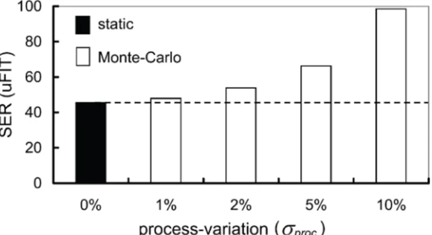
Using the 45nm Predictive Technology Model (PTM) [24], the impact of process variations on circuit reliability is illustrated in Figure 1.2, where SERs are computed by SPICE simulation on a sample circuit c17 from ISCAS 85 under different values (σproc’s) of process variation applied to perturbing separately the gate width and channel length of each transistor in each cell’s geometry. The X-axis and Y-axis denote σproc and SER, respectively, where FIT (Failure-In-Time) is defined by the number of failures per 109 hours. Nominal settings without variation are used in static SPICE simulation, whereas Monte-Carlo SPICE simulations are used to approximate process-variation impacts under different σproc’s.
As a result, SER from static SPICE simulation is underestimated. Considering different σproc’s in Monte-Carlo SPICE simulation, all SERs are higher than that from static SPICE simulation. As process variations deteriorate, the discrepancy between
Monte-Carlo and static SERs further enlarges. In Figure 2, (SERmonte –SERstatic)/SERstatic under σproc = 1%, 2%, 5% and 10% are 6%, 19%, 46% and 117%, respectively. Such result suggests that the impact of process variations to SER analysis may no longer be ignored in scaled CMOS designs.
Figure 1.2: SER discrepancies between static and Monte-Carlo SPICE simulation w.r.t. process-variation
1.1 Research goal
In this project, we formulate the statistical soft error rate (SSER) problem and present three frameworks to cope with the aforementioned sophisticated issues. We first review statistical soft error rate analysis based on which a Monte-Carlo framework is built. We further employ the quasi-random sequences, which successfully speeds up the convergence of simulation error and shortens the runtime. Moreover, advanced sampling techniques are incorporated for variance reduction of SSERs. Then, SVR-learning framework captures the change of transient-fault distributions explicitly using statistical learning theory. Regardless of the methods used, current statistical SER (SSER) frameworks invariably involve a trade-off between accuracy and efficiency. Third framework presents accurate cell models in first-order closed-form to overcome this problem, thereby enabling the analysis of SSERs in a block-based fashion similar to statistical static timing analysis (SSTA).
1.2 Research method
1.2.1 First year
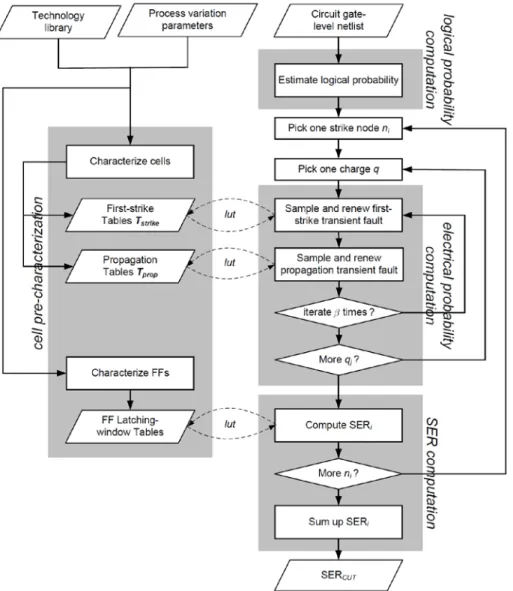
Monte-Carlo (MC) method, a computational algorithm using repeated random samplings to portray complex statistical behaviors of physical or mathematical systems as depicted in Figure 1.3. This framework maps to the three masking mechanism using three loops: the outmost loop considers various levels of collection charge; the second loop accounts for all vulnerable nodes within a circuit; the innermost loop computes δstrike and δprop implicitly. As the key component of the framework, the last loop can be further decomposed into two parts: (1) cell pre-characterization and (2) sampling and renewal of transient faults.
Figure 1.3: Proposed table-lookup framework
Furthermore, we customize the use of quasi-random sequences, which successfully speed up the convergence of simulation error and hence shorten runtime. However, there is still a problem about the uniformity of the quasi-sequence samples in multivariate distribution. To solve this problem, we use importance sampling to
reduce variance in quasi-sequence samples. From experimental results, the framework is capable of yielding more accurate SSER results compared to previous works and running much faster.
1.2.2 Second year
Integrating the impact of process variations, four models are traditionally built using lookup tables. However, lookup tables have two limitations on applicability: (1) inaccurate interpolation and (2) coarse model-size control. First, lookup tables can take only finite table indices and must use interpolation. However, interpolation functions are often not accurate enough or difficult to obtain, especially as the table dimensionality grows. Second, a lookup table stores data samples in a grid-like fashion, where the table will grow prohibitively large for fine resolution. Meanwhile, the information richness often differs across different parts of a table. For example, we observe that pulse widths generated by strong charges behave much simpler than weaker charges do. Naturally, simple behaviors can be encoded with fewer data points in the model, whereas complicated behaviors need to be encoded with more.
In this year, we proposed another learning-based framework to computes δstrike and δprop directly with support of support vector regression (SVR) and is found to be both more efficient and more accurate than table look-up method. Note that our SVR-learning framework can be represented in the same flowchart as Figure 1.3 with the replacement of first-strike tables (Tstrike) and propagation tables (Tprop) with respective learning models (δstrike and δprop).
1.2.3 Third year
In this year, we proposed a novel approach, similar to that of block-based SSTA, for SSER in which a transient fault is decomposed into two transitions for analysis: a rising edge and a falling edge. Each edge is processed using an analytical approach and statistical static timing analysis, which is based on a first-order closed-form. Because the transient fault is analyzed using a mathematical method, the timing cost can be largely reduced and timing information can be preserved, which is helpful for describing the interactive behavior of transient faults. However, correlations are the main concern when applying a closed-form block-based approach to the estimation of SSER. Theoretically, all correlations between transition signals and corresponding gate delays must be considered; however, the correlation between transition signals can be overlooked because the difference in SER has been shown to be less than 1%
according to our experiments. Thus, we devised a parameterized SSTA framework that takes into account the timing correlation to derive more accurate SER. Experimental results demonstrate that our approach can provide reasonable results much more rapidly than all previous works.
Chapter 2
Fundamental of Statistical Soft Error Rate
2.1 Transient-fault behavior in very deep submicron era
Transient faults exhibit two characteristics in the very deep sub-micron era. One makes the faults more unpredictable whereas the other causes the discrepancy in Figure 1.2. In this section, the discrepancy are explained and associated with the electrical and timing masking mechanisms, respectively
2.1.1 To be electrically better or worse?
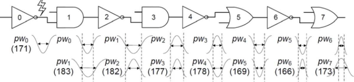
The first observation is conducted by running static SPICE simulation on a path consisting of various gates (including 2 AND, 2 OR and 4 NOT gates) in the 45nm PTM technology. As shown in Figure 2.1, the radiation particle first strikes the output of the first NOT gate with a collection charge of 32fC, and then propagates the transient fault along other gates with all side-inputs being set properly. The pulse widths (pwi’s) in voltage of the transient fault starting at the struck node and after passing gates along the path in order are 171ps, 183ps, 182ps, 177ps, 178ps, 169ps, 166ps and 173ps, respectively. Each pwi and pwi+1 can be compared to show the changes of voltage pulse widths during propagation in Figure 2.1.
Figure 2.1: Static SPICE simulation of a path in the 45nm technology
As we can see, the voltage pulse widths of such transient fault grow larger through gate #1, #4, and #7 while gate #2, #3, #5 and #6 attenuate such transient fault. Furthermore, gates of the same type behave differently when receiving different voltage pulses. To take AND-type gates for example, the output pw1 is larger than the input pw0 on gate #1 while the contrary situation (pw3 < pw2) occurs on gate #3. This
result suggests that the voltage pulse width of a transient fault is not always diminishing, which contradicts some assumptions made in traditional static analysis [10]. A similar phenomenon called Propagation Induced Pulse Broadening (PIPB) is discovered in [25] and states that the voltage pulse width of a transient fault widens as it propagates along the long inverter chain.
2.1.2 When error-latching probability meets process variations
The second observation is dedicated to the timing-masking effect under process variations. In [9][18], the error-latching probability (PL) for one flip-flop is defined as
PL =pw−wt
clk (1)
where pw, w and tclk denote the pulse width of the arrival transient fault, the latching window of the flip-flop, and the clock period, respectively. However, process variations make pw and w become random variables. Therefore, we need to redefine Equation (1) as following.
Definition (Perr−latch, error-latching probability)
Assume that the pulse width of one arrival transient fault and the latching window (tsetup+thold) of the flip-flop are random variables and denoted as pw and w,
respectively. Let x = pw − w be another random variable and μx and σx be its mean
and variance. The latch probability is defined as:
Perr−latch(pw, w) =t1
clk∫ x ∙ P(x > 0) ∙ 𝑑𝑑
ux+3σx
0 (2)
With the above definition, we further illustrate the impact of process variations on SER analysis. Figure 4(a) shows three transient-fault distributions with the same pulse-width mean (95ps) under different σproc’s: 1%, 5% and 10%. A fixed latching window w = 100ps is assumed as indicated by the solid lines. According to Equation (1), static analysis result in zero SER under all σproc’s because 95 − 100 < 0.
From a statistical perspective, however, these transient faults all yield positive and different SER’s. It is illustrated using two terms: P(x > 0) and x in Equation (2). First, in Figure 2.2(a), the cumulative probabilities for pw > w under three different σproc’s are 17%, 40%, and 49%, respectively. The largest σproc corresponds to the
largest P(x > 0) term. Second, in Figure 2.2(b), we compute the pulse-width averages for the portion x = pw − w > 0 and they are 1, 13 and 26, respectively. Again, the largest σproc corresponds to the largest x term.
These two effects jointly suggest that larger σproc leads to larger Perr−latch, which has been neglected in traditional static analysis, and also explain the increasing discrepancy shown in Figure 1.2. In summary, process variations make traditional static analysis no longer effective and should be considered in accurate SER estimation for scaled CMOS designs.
Figure 2.2: Process-variation vs. error-latching probabilities
2.2 Impact of spatial correlation
Variations have become important as technology scales further. High levels of device parameter variations are changing the design flows from deterministic to probabilistic as technology nodes beyond 90nm experience increasingly. Process variations can be classified into the two categories. One is the inter-die variations and the other is intra-die variations. Intra-die variations can significantly affect the variability of performance parameters on a chip due to the modern technologies are rapidly and steadily growing. Intra-die variations are locally layout-dependent, and
therefore it is spatially correlated.
Devices tend to have similar characteristics as it with similar layout patterns and proximity structures. In other words, it is globally location-dependent. Devices have the similar characteristics than placed far away as it located close to each other. With increased process scaling, intra-die variations are becoming a more dominant portion of the overall variability of device features, meaning that devices on the same die can no longer be treated as identical copies of the same device.
If we do not take into account the value of process variations, it will lead to underestimated/overoptimistic estimation on SSER. However, all previous works consider the impact of process variations but do not include spatial correlations in the statistical soft error rate, leading to incorrect SSERs. Therefore, we investigate the impact of spatial correlations in our project to comprehend the accuracy of SSERs as shown in Figure 2.3.
Figure 2.3: SSER comparison from static and Monte Carlo SPICE simulations, the proposed MC with spatial correlations and without spatial correlations frameworks
According to Figure 2.3, circuit SER is overestimated under the process variation 5% without considering spatial correlations. Circuit SER that considers spatial correlations under the process variation 5% is generally lower when comparing with the circuit SER under the process variation 5% without considering spatial correlations. Therefore, we propose an effective model considering spatial correlations of statistical soft error rate. The analysis is extended to include spatial
correlations. Then we explain the model used for process variations and spatial correlations of intra-die variations.
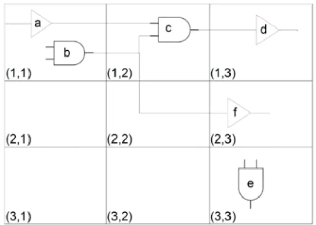
There are a few models in order to handle parameter correlations. First, we introduce the grid model. Grid model is a die area divided by a square grid. A group of fully correlated devices is assumed to correspond to each square of the grid. Each square is modeled as a random variable (RV) which correlates with the random variables corresponding to the rest of the squares. Another one model is called the quadtree model. This method is recursively dividing the die area into four squares until individual gates into the grid. The partitions are stacked on top of another level. We then assign each of them an independent random variable. By summing all areas that cover this particular device, the random variable corresponding to the gate is computed. Due to share common random variables on higher levels, the spatial correlations can be addressed properly.
Without losing the generality, in the beginning of our project, we used the grid model to apply spatial correlations to soft error. We partitioned the region of die into nrow*ncol = n2 grids for modeling the intra-die spatial correlations of parameters. We assumed that perfect correlations among the devices are in the same grid. Low or zero correlations are between far-away grids, and high correlations between close grids. The devices are more likely to have more similar characteristics than those placed far away due to they are close to each other. For example, Figure 2.4 shows that gate a in grid (1, 1) and gate e in grid (3, 3). Since they are far away from each other, we assume that their parameters are uncorrelated. Gate c in grid (1, 2), gate a and gate c lie in neighboring grids, and due to their spatial proximity, their parameter variations are not identical but should be highly correlated. Since gate a and gate b are located in the same grid, we assume that the variations of their gate length are identical.
Our algorithm makes a second assumption. Assume that there are no correlations between different types of process parameters, and nonzero correlations may exist only among the same type of process parameters in different grids. For instance, the Lg values for transistors in nearby grids are correlated, but the other parameters such as Wg or Wint in any grid are uncorrelated. In other words, we assume that interconnect parameters in different layers to be different types of parameters.
2.3 Full-spectrum analysis or not
Some previous works simplify the SER estimation by injecting only four levels of electrical charges. Therefore, our project poses a simple, yet important question,
“Are four levels of electrical charges enough to converge SER correctly and properly address the process-variation effect?”
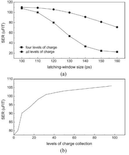
Figure 2.5: (a) SERs of four-level and full-spectrum charge collection w.r.t. different latching-window size (b) SERs w.r.t. different levels of charge collection
Figure 2.5(a) compares of SERs from Monte-Carlo SPICE simulations. These SERs had different levels of charges when collected onto a sample circuit (c17 from ISCAS’85) with different latching-window sizes. The line with square symbols and the line with circle symbols represent the SERs induced by four-level and full-spectrum charge collection, respectively. As the latching-window size was set to 100ps, the SERs obtained from four-level and full-spectrum analyses were the same. However, as the latching-window size grew to 150ps, the effective range of charge collection for SSER analysis increased from 35fC to 132fC. Therefore, the SER difference between four-level and full-spectrum analyses grew to 69%. Another question naturally arises, “If four levels of charge collection are not sufficient to
derive accurate SERs, how many levels are sufficient?”
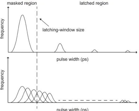
Figure 2.6: Transient-fault distributions induced by four-level and full-spectrum charge collection
Figure 2.5(b) suggests the answer. All levels of deposited charges should be considered because SERs increase with charge collections. SER difference using different levels of deposited charges is further illustrated (Fig. 2.6), where the upper and lower parts show SER estimation by only four levels of charges and by all levels of charges, respectively. The X-axis and Y-axis denote the pulse width of transient faults and the effective frequency for a particle strike of different levels of deposited charges. For the analysis using four-level deposited charges, only four transient-fault (TF) distributions were generated and could contribute to the final soft error rate. In other words, soft errors can only be generated from four concentrated distributions,
and therefore may result in mistakes on SER integration. As the latching-window size of one flip-flop was far from the first TF distribution, soft errors from such TF distributions were entirely masked due to the timing-masking effect. For example, the biggest pulse width distribution in the upper part of Figure 2.6 is excluded from SER estimation. But, only part of them (those smaller decomposed TF distributions) were masked during analysis using all levels of deposited charges (Figure 2.6, lower part). As a result, SER estimation was no longer valid with analysis using only four levels of charges and instead should comprehensively consider full-spectrum charge collection.
2.4 Problem formulation of statistical soft error rate (SSER)
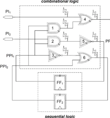
In this section, we formulate the statistical soft error rate (SSER) problem for general cell-based circuit designs. Figure 2.7 illustrates a sample circuit subject to process variations, where the geometries of each cell vary [21]. Once high-energy particles strike the diffusion regions of these variable-size cells, according to Figure 1.2, 2.1 and 2.2, the electrical performances of the resulting transient faults also vary a lot. Accordingly, to accurately analyze the soft error rate (SER) of a circuit, we need to integrate both process-variation impacts and three masking affects discussed in Chapter 1 simultaneously, which brings up the statistical soft error rate (SSER) problem.
The SSER problem is composed of three elements: (1) electrical-probability computation, (2) propagation-probability computation and (3) overall SER estimation. A bottom-up mathematical explanation of the SSER problem will start reversely from overall SER estimation to electrical probability computation.
2.4.1 Overall SER estimation
The overall SER for the circuit under test (CUT) can be computed by summing up the SER’s of each individual node in the circuit. That is,
𝑆𝑆𝑆
𝐶𝐶𝐶= ∑
Ni=0nodeSER
i(3)
where Nnode denotes the total number of possible nodes to be struck by radiation particles in the CUT and SERi denotes the SER results from node i, respectively.
Each SERi can be further formulated by integrating over the range q = 0 to Qmax (the maximum collection charge from the environment) the products of particle-hit rate and the total number of soft errors that q can induce at node i. Therefore,
SERi = ∫q=0Qmax(Ri(q) × Fsoft−err(i, q))dq (4)
In a circuit, Fsoft−err(i, q) represents the total number of expected soft errors from each flip-flop that a transient fault from node i can propagate to. Ri(q) represents the effective frequency for a particle hit of charge q at node i in unit time according to [1][8]. That is,
𝑆𝑖(q) = F × K × Ai×Q1se
−q
Qs (5)
where F, K, Ai and Qs denote the neutron flux (> 10MeV), a technology-independent fitting parameter, the susceptible area of node i in cm2, and the charge collection slope, respectively.
Fsoft−err(i, q) depends on all three masking effects and can be decomposed into
Fsoft−err(i, q) = ∑ PNj=0ff logic(i, j)× Pelec(i, j, q) (6)
where Nff denotes the total number of flip-flops in the circuit under test. Plogic(i, j) denotes the overall logical probability of successfully generating a transient fault and propagating it through all gates along the path from node i to flip-flop j. It can be computed by multiplying the signal probabilities for specific values on target gates as follows.
𝑃𝑙𝑙𝑙𝑖𝑙(i, j) = Psig(i = 0) × ∏k∈i→jPside(k) (7) where k denotes one gate along the target path (i→j) starting from node i and ending at flip-flop j, Psig denotes the signal probability for the designated logic value, and Pside denotes the signal probability for the non-controlling values (i.e. 1 for AND gates and 0 for OR gates) on all side inputs along the target path.
Figure 2.8 illustrates an example where a particle striking net a results in a transient fault that propagates through net c and net e. Suppose that the signal probability of being 1 and 0 on one arbitrary net i is Pi and (1-Pi), respectively. In order to propagate the transient fault from a towards e successfully, net a needs to be 0 while net b, the side input of a, and net d, the side input of c, need to be non-controlling, simultaneously.
Figure 2.8: Logical probability computation for one sample path
Therefore, according to Equation (7),
𝑃𝑙𝑙𝑙𝑖𝑙(a, e) = Psig(a = 0) × Pside(a) × Pside(c)
= Psig(a = 0) × Psig(b = 1) × Psig(d = 0) = (1 − Pa) × Pb× (1 − Pd)
2.4.3 Electrical probability computation
Electrical probability Pelec(i, j, q) comprises the electrical and timing masking effects and can be further defined as
𝑃𝑒𝑙𝑒𝑙(i, j, q) = Perr−latch�pwj, wj�
= Perr−latch�𝜆elec−mask(i, j, q), wj� (8) While Perr−latch accounts for the timing making effect as defined in Equation (2), λelec−mask accounts for the electrical masking effect with the following definition.
Definition (λelec−mask, electrical masking function)
Given the node i where the particle strikes to cause a transient fault and flip-flop j is the destination that the transient fault finally ends at, assume that the transient fault propagates along one path (i ; j) through v0, v1, ..., vm, vm+1 where v0 and vm+1 denote
node i and flip-flop j, respectively. Then the electrical masking function is defined as
𝜆elec−mask(i, j, q) = δprop�⋯ �δprop�δprop(pw0, 1), 2�, ⋯ �, m, � (9) where pw0 = δstrike(q, i) and pwk = δprop(pwk−1, k) ∀k ∈ [1,m]
In the above definition, two undefined functions, δstrike and δprop, respectively, represent the first-strike function and the electrical propagation function of transient-fault distributions. δstrike(q, i) is invoked once and maps the collection charge q at node i into a voltage pulse width pw0. δprop(pwk−1, k) is invoked m times and iteratively computes the pulse width pwk after the input pulse width pwk−1 propagates through the k-th cell from node i. These two types of functions are also the most critical components to the success of a statistical SER analysis framework due to the difficulty from integrating process-variation impacts.
The theoretical SSER in Equation (7) and Equation (9) is analyzed from a path perspective. However, in reality, since both the signal probabilities and transient-pulse changes through a cell are independent to each other, the computation of SSER only needs to proceed stage by stage and thus can be implemented in a block-based fashion. Chapter 3, Chapter 4 and Chapter 5 will present three different block-based SSER frameworks, a table-lookup framework, SVR learning framework, and SSTA-like framework, respectively. These frameworks consider process variations but differ
Chapter 3
Table-lookup Monte-Carlo (MC)
Framework
The first framework combines the current static approaches with the Monte-Carlo (MC) method, a computational algorithm using repeated random samplings to mimic complex statistical behaviors of physical or mathematical systems. As depicted in Figure 1.3, this framework maps to the formulation in Section 2.4 using three loops: the outmost loop considers various levels of collection charge qi, which forms the discrete approximation of Equation (4); the second loop accounts for all vulnerable nodes within a circuit, which corresponds to Equation (6); the innermost loop maps to Equation (9) and computes δstrike and δprop implicitly. As the key component of the framework, the last loop can be further decomposed into two parts: (1) cell pre-characterization and (2) sampling and renewal of transient faults.
3.1 Cell pre-characterization
To reflect the electrical masking effect of transient faults on one cell intertwined with process variations, an approach similar to [26] is employed to extract pre-characterized tables. The objective of such pre-characterized tables is to model the pulse width and voltage magnitude for each cell as random variables that can be sampled during the particle-strike process and transient-fault propagation of one cell.
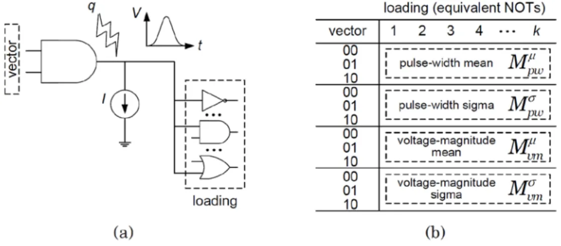
Table contents are derived on the basis of data from Monte-Carlo SPICE simulation with targeted process-variation parameters (or direct silicon measurement on test structures if applicable). Considering the mapping relationship, two types of tables are built for each cell separately: one for the particle-strike process, Tstrike, and the other for transient-fault propagation, Tprop
3.1.1 Particle-strike table T
strikeTstrike maps the collection charge q incurred by the particle strike to electrical properties of cells. Figure 3.1 illustrates the example to pre-characterize one AND gate by properly setting up SPICE simulation environment. Figure 3.1(a) is the circuit netlist where a charge q is injected at the output of the AND gate as an independent
current source according to [7]:
I(q, t) =𝜏 q
𝛼−𝜏𝛽× (e
−𝜏𝛼t − e−𝜏𝛽t)
(10)
An arbitrary number of cells are also generated and connected as the output loading for the AND gate. Capacitance of each cell will be normalized in terms of the unit-size inverter (NOT). The final output loading is obtained from summing up each output cell and represented by a total number of equivalent NOTs.
Figure 3.1: Pre-characterization of particle-strike table Tstrike for an AND gate
Given a fixed q, a number of MC runs with different SPICE settings are repeated in Figure 1.3 to compute the means and variances of pulse width and voltage magnitude, respectively, for the resulting transient fault. Figure 3.1(b) shows the table for the AND gate including four matrices: pulse-width mean matrix (Mpwμ ), pulse-width variance matrix (Mpwσ ), voltage-magnitude mean matrix (Mvmμ ) and voltage-magnitude variance matrix (Mvmσ ) to store mean and sigma values for pulse widths and voltage magnitudes of transient-fault propagation. Note that since first-strike transient faults are sensitive to input vectors, the input vector also serves as an index in Tstrike.
3.1.2 Transient-fault propagation table T
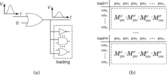
propThe transient-fault propagation table Tprop, on the other hand, reflects the changes of electrical properties when propagating the transient fault through one cell. Figure 3.2(a) shows the sample SPICE simulation environment to pre-characterize the transient-fault propagation through one OR gate. The output loading is set up
similarly to the pre-characterization of Tstrike for the AND gate mentioned above. Both input and output of the OR gate are described as glitches and pulse widths and voltage magnitudes are measured accordingly.
Figure 3.2: Pre-characterization of transient-fault-propagation table Tprop for OR gate
After performing statistical calculation, four matrices, pulse-width mean (Mpwμ ), pulse-width sigma (Mpwσ ), voltage-magnitude mean (Mvmμ ) and voltage-magnitude sigma (Mvmσ ) can be obtained for one output loading in the tables. Furthermore, each Tprop has three dimensions where the first one is the output loading (load = 1..k), the second one is the input pulse width (pw0...pwm), and the third one is the input voltage magnitude (vm0...vmn). Therefore, the above process iterates k times to derive one Tprop of size 4 × k × m× n.
3.2 Sampling and renewal of transient faults
Each Monte-Carlo (MC) run consists of two types of actions: sampling and renewal. A two-tuple transient fault f=(pw,vm) is first generated by randomly choosing pw and vm from pulse-width and voltage-magnitude distributions in Tstrike according to the probability theory. Later, electrical properties of f after propagating through the next cell are renewed and new pulse-width and voltage-magnitude distributions can be looked up from Tprop of such cell. Then a sampling step repeats to
pick next f′ = (pw′, vm′) followed by looking up the next (μpw′ , σpw′ ) and (μvm′ , σ
vm
′ ) in the renewal step. The sampling and renewal steps alternate until the transient fault either reaches the input of any flip-flop or disappears during its propagation.
Transient-fault probability P(f) denotes the updated probability after f propagates through one gate and is also incorporated in the proposed table-lookup framework. Initially, all inputs are assumed to be a independent variable with equal probabilities of being 1 and 0. Probabilities for each node can be derived statically according to its input probabilities. Later, during computing the change of f on each cell, P(f) is updated simultaneously to reflect the logic masking effect mentioned in Section 2.4. Two different cases are discussed in detail as follows.
3.2.1 First-strike cases
For the first-strike cases, the struck node is required to remain 0 for a positive transient fault and 1 for a negative transient fault. Let’s take one AND gate shown in Figure 3.3(a) for example. Given the collection charge q, transient fault fz = (pwz, vmz) can be looked up in Tstrike and denoted as fz= lutP.S.(q, z). Assume that the probabilities of being 1 for input x and y are denoted by Px and Py. For the particle strikes the output z to induce a positive transient fault (fz+), z is required to be 0 and thus, P(fz+) = (1 − Px) × Py. Similarly, for a negative transient fault (fz−) striking output z, P(fz−) = Px × Py.
Figure 3.3: Logical probability update for an AND gate
3.2.2 Propagation cases
For the propagation cases, in order to propagate the positive (or negative) transient fault through one gate, all other side-inputs are required to be non-controlling values (n.c.v.). Besides, non-convergent and convergent conditions need to be considered separately. Figure 3.3(b) illustrates a non-convergent example
of the AND gate. Similarly, given fx, fz can be looked up in Tprop by
fz = lutprop.(fx, z) = (pwz, vmz . As to transient-fault probability, since
non-convergent condition assumes that only one positive (or negative) transient fault arrives one input of the AND gate, say x in this example, only y is required to be 1 (n.c.v. for the AND gate). Therefore, P(fz) = P(fx) × Py.
A transient fault going through multiple propagation paths may re-converge to one node, which is very expensive to handle using enumeration. Currently, the worst-case approximation is used since it is reported to have only minor estimation error. From the electrical perspective, the worst case denotes a re-convergent transient fault that has the maximum pulse-width and voltage magnitude among updated values from each input transient faults. An example for the AND gate is shown in Figure 3.4(a). Following this notion, a MAX operation is defined to facilitate such computation:
fz = MAX �lutprop(fx), lutprop�fy��
= MAX �lutprop(pwx, vmx), lutprop�pwy, vmy�� = MAX �(pwx′, vmx′), �pwy′, vmy′��
= MAX ��pwx′, pwy′�, �vmx′, vmy′��
= pwz, vmz (11)
where lut() looks up values from Tprop in the renewal step.
Figure 3.4: Re-convergent transient faults on an AND gate
From the logical perspective, the worst case happens when the arrival windows of two transient pulses are not overlapped and Figure 3.4(b) illustrates this concept. The corresponding transient-fault probability P(fz) can be computed by the summation of two transient-fault probabilities from input x and y. That is,
3.3 Using qauasirandom sequences
Pseudorandom number generation plays a key role to the success of the Monte Carlo method. However, using rand() function for sampling points often suffers from the clustering problem in high dimensional spaces. Figure 3.5(a) illustrates this problem on an example of generating a (X, Y)-distribution by the Mont e Carlo method using the rand() function . The sampling points are observed not evenly scattered among the (X, Y) plate, which means that these sampling points from pseudorandom generation may not be representative enough for the entire space.
Figure 3.5: Distributions from the Monte Carlo methods with random number generation and quasirandom sequences
The clustering problem motivates research of finding a deterministic sequence such that well-chosen points are distributed in the high-dimensional spaces uniformly. Such sequences are named quasirandom sequences. Figure 3.5(b) shows the same number of sampling points using quasirandom sequences on the (X,Y) plate. Sobol algorithm is used to generate the corresponding sequences. From Figure 5(b), new sampling points are observed more uniformly distributed over the (X,Y) plate and thus have better representativeness.
Monte Carlo methods with quasirandom sequences are termed Quasi-Monte Carlo (QMC) methods. Given a sampling number N and a dimension d, Monte Carlo methods converge with O(1/√N) simulation errors whereas QMC methods converge with O(1/√N) for optimal cases. Previous research works have demonstrated better
results for QMC than MC methods for t he problems with ≤360 dimensions in
Since each gate in the circuit becomes a free dimension (regardless of spatial correlations) , the total dimension in the corresponding SSER system can be very high . However, for a large d and moderate N, quasirandom sequences perform no better than the pseudorandom sequences. Besides, high dimensional quasirandom sequences tend to suffer from the clustering problem again. In the worst cases, QMC’s convergence rate,O((lnN)d/N), are even worse than MC's O(1/√N) as d goes larger . Therefore, we are motivated to apply dimension reduction to ensure the effectiveness of the proposed QMC framework for SSER analysis.
Effective dimensions of circuits can be observed through experiment s. Figure 3.6 shows the convergence rates for four sample circuit s where the vertical lines indicate the logic depths (a.k.a. levels) of each circuit. All convergence rates drop quickly as the dimension numbers increase. Such phenomenon implies their underlying SSER systems can be properly described using much lower dimensions. For example, the intuitive dimension number for the circuit c7552 is 2114, the total number of its nodes. From Figure 3.6(d), however, a dimension number of 60 is already good enough. Also, from Figure 3.6 states that the circuit level can suffice to represent the total dimension and thus converge SER faster.
3.4 Applying importance sampling on QMC
In this project, we also combine the QMC and importance sampling in order to efficiently calculate expectations with respect to multivariate distributions. This method can be used to circumvent the definition of non-uniform quasi-random varieties. Interpreted as a parameter transformation method, it can get rid of singularities of the integrand which increases the speed of convergence of QMC. In the case of complicated multivariate distributions the application of QMC techniques is much easier for importance sampling than for Markov chain Monte Carlo methods.
3.4.1 Importance sampling overview
In importance sampling, one attempts to avoid taking samples in regions where the value of the function is negligible, and to focus on regions where the value is large. It is important to allow for this bias in sampling by weighting the sample values appropriately. Importance sampling is based on the idea of using weights to correct for the fact that we sample from the instrumental distribution g(x) in place of the target distribution f(x). Importance sampling is based on the identity shown as follows: ( ) ( ) ( ) ( ) ( ) ( ) ( ) x x x f x P X x f x dx g x dx g x w x dx g x ∈
∫
=∫
=∫
For all g(x), such that g(x) > 0 for (almost) all x with f(x) > 0. We can generalize this identity by considering the expectation Ef (h(X)) of a measurable function h:
( ) ( ( )) ( ) ( ) ( ) ( ) ( ) ( ) ( ) ( ( ) ( )) ( ) f g f x E h X f x h x dx g x h x dx g x w x h x dx E w X h X g x =
∫
=∫
=∫
= ⋅Importance sampling is a numerical method in order to approximate an integral. It can be implemented to estimate the mean response for a given sample under an alternate distribution. Importance sampling is based on the following identity. Let G and g be the distribution function and the density function of some distribution, called importance distribution in the sequel as following equation:
( ) ( ) ( ) ( ) ( ) ( ) ( ) ( ) ( ) ( ) d d d f q R R R f x E q x f x dx q x g x dx q x w x dG x g x =
∫
=∫
=∫
The importance distribution can be chosen such that it is not hard to generate a sample of points that follow the importance density. In the case of QMC this will be the inversion method. In dimension one (d = 1), we then have the estimator:
1 1 ( ) (0,1)
( ) ( )
(
())
(
( ))
d f q RE
=
∫
q x f x dx
=
∫
q G
−⋅
w G
−u du
By a proper choice of the importance density g, the integrand has bounded variation. It is enough that g has higher tails than the product of q(x)f(x) to get rid of the singularity problem.
Algorithm 3-1 (importance sampling): 1. for i = 1 to n generateXi fromg X( ); let
(
)
(
)
(
)
i i if X
w X
g X
=
; 2. return 1 1 ( ) ( ) ˆ ( ) n i i i n i i w X h X u w X = = ⋅ =∑
∑
;The following theorem, bias and variance of Importance Sampling, gives the bias and the variance of importance sampling.
(a)
E u
g( )
=
u
(b)var ( ( )
( ))
var ( )
gu
gw X
h X
n
⋅
=
The theorem implies that contrary to µ� the self-normalized estimator µ� is biased. The self-normalized estimator µ� however might have a lower variance. In addition, it has another advantage: we only need to know the density up to a multiplicative constant, as it is often the case in hierarchical Bayesian modeling.
3.4.2 Advantage of applying importance sampling on QMC
integration: the integrand can have singularities when the domain of the distribution is unbounded and it can be very expensive or difficult to sample points from a general multivariate distribution. ( )
( ) ( )
( )
( )
d d f q R RE
=
∫
q x f x dx
=
∫
q x dF x
For typical applications, we want to derive expectation, variance and some quantities of all marginal distributions together with all correlations between the variables. If we consider, for instance, the expectation, it is obvious that we have to use q(x) = xk to obtain the expectation of the marginal.
The convergence rate often can be increased when highly uniform point sets (HUPS, also called low discrepancy sequences or quasi-random numbers) are used instead of (pseudo-) random points. Such methods are called quasi-Monte Carlo methods (QMC). There exist HUPS where the star discrepancy (and thus the QMC estimator) converges withO((lnN)d/N). When E f (q) has to be evaluated with respect to some non-uniform distribution F with bounded domain, similar results exist.
The QMC approach requires point sets with low F–discrepancy. Such point sets are also created by applying appropriate transformation methods on low discrepancy sequences. However, for general multivariate distributions such transformations are hard to find and/or numerically very expensive. Moreover, these may introduce singularities into our integration problem and thus convergence is not guaranteed by the Koksma-Hlawka inequality.
Thus, we need to transform low discrepancy point sets into sets of points with low F-discrepancy when we calculate the QMC estimator. However, the transformation methods that have been developed for non-uniform random variety generation cannot be applied for QMC, because these destroy the structure of the underlying point set. Moreover, the theory of non-uniform random numbers does not directly apply when quasi-random numbers are used.
The problem of generating non-uniform random points and that of generating non-uniform quasi-random points should be seen as different problems. For the first one, we need to transform uniform random numbers into random points. The correctness of the transformation is verified using probability theory. The structure of the used uniform pseudo-random point set is usually not taken into consideration. The
latter problem of generating quasi-random points should be interpreted as transforming the integration problem with respect to F over Rd into an equivalent one over (0, 1) with respect to the Lebesgue measure. This is required as HUPS are constructed to work for the integral over the unit cube. From this perspective, it is somewhat surprising that most papers dealing with QMC methods for evaluating expectations E f (q) do not concern about the problem of appropriate transformations.
There are some problems with this approach. First, the inverse CDF, F−1, is often not given in closed form and thus numerical methods that only compute F−1(u) approximately have to be used. There exist fast methods for this task, but they either require the CDF or compute it by integrating the density function numerically. In the multivariate case the inversion method can be applied to the marginal distributions, if the components of the random vector X are stochastically independent. Otherwise, the conditional distribution method must be used which can be seen as the multivariate generalization of the inversion method. It needs the (inverse) CDF of conditional distributions of marginal distributions which is practically never available in practice. Moreover, the F-discrepancy is increased when the components are not independent.
A more serious problem in the framework of QMC is the fact that the inter-grand q(F−1(u)) is often unbounded and thus has unbounded variation when the support of the distribution is unbounded. This is for instance the case when the m-th moment of the i-th variable has to be computed in Bayesian inference where q(x) = xim or in derivative pricing in financial engineering when q(x) behaves like exp (∑ xid
i=1 ). In this case the Koksma-Hlawka inequality does not apply and convergence of the QMC estimator is not guaranteed.
Chapter 4
Support-Vector-Regression (SVR) Learning
Framework
The table-lookup Monte-Carlo framework is inherently limited in execution efficiency because it computes δstrike and δprop indirectly using extensive samplings of Monte-Carlo runs. In this section, we propose another learning-based framework to do the task directly with support of support vector regression (SVR) and is found to be both more efficient and more accurate. Note that our SVR-learning framework can be represented in the same flowchart as Figure 1.3 with the replacement of first-strike tables (Tstrike) and propagation tables (Tprop) with respective learning models (δstrike and δprop) as shown in Figure 4.1.
Figure 4.1: Proposed statistical SER framework using support-vector-regression models
By definition, δstrike and δprop are functions of pw that is a random variable. From Figure 2.1 and Figure 2.2, we assume pw follows the normal distribution, which can be written as:
pw~N(μpw, σpw) (13) Therefore, we can decompose δstrike and δprop into four models: δstrikeμ , δstrikeσ , δpropμ , and δpropσ where each can be defined as:
δ: x�⃗ → y (14) where x�⃗ denotes a vector of input variables and y is called the model’s label or target value
Integrating the impact of process variations, four models are traditionally built using lookup tables. However, lookup tables have two limitations on applicability: (1) inaccurate interpolation and (2) coarse model size control. First, lookup tables can take only finite table indices and must use interpolation. However, interpolation functions are often not accurate enough or difficult to obtain, especially as the table dimensionality grows. Second, a lookup table stores data samples in a grid-like fashion, where the table will grow prohibitively large for fine resolution. Meanwhile, the information richness often differs across different parts of a table. For example, we observe that pulse widths generated by strong charges behave much simpler than weaker charges do. Naturally, simple behaviors can be encoded with fewer data points in the model, whereas complicated behaviors need to be encoded with more.
In statistical learning theory, such models are built using regression, which can be roughly divided into linear [27] and non-linear [28] methods. Among them, Support Vector Regression (SVR) [29] [30] combines linear methods’ efficiency and non-linear methods’ descriptive power. SVR has two advantages over lookup tables: (1) It gives an explicit function and need no interpolation. (2) It filters out unnecessary points and yields compact models. In the following, we propose a methodology to adapt the framework in Chapter 3 to a learning-based one based on SVR models, which comprises training sample preparation, SVR model training, and parameter selection. Also, the modification of the MAX operation in Equation (11) is addressed.
4.1 Training sample preparation
SVR models differ from lookup tables on the way we prepare training samples for them. For lookup tables, one starts from selecting a finite set of points along each table dimension. On one hand, they should be chosen economically; on the other hand, it is difficult to cover all corner cases with only a limited numbers of points. For SVR models, we do not need to select these points. Instead, we provide large sets of training samples, and let the SVR algorithm do the selection task.
A training sample set S of m samples is defined as:
S ∈ (X��⃗ × Y)m = {(x�⃗
1, y1), ⋯ , (x�⃗m, ym)} (15) where m pairs of input variables x�⃗i’s and target values yi’s are obtained from massive Monte-Carlo SPICE simulation. For δstrikeμ , δstrikeσ , we use input variables including charge strength, driving gate, input pattern, and output loading; for δpropμ , δpropσ , we use input variables including input pattern, pin index, driving gate, input pulse-width distribution ( μpwi−1 and σpwi−1 ), propagation depth, and output loading.
In our training samples, we implement output loading using combinations of arbitrary cell input pins. Doing so preserves additional information for the output loading status and saves the labor (and risk) of characterizing the capacity of each cell’s input pin. Although the number of such combinations can easily explode, there are usually only a limited number of representatives, which are automatically identified by SVR. Furthermore, from a learning perspective, since both peak voltage and pulse width are the responses of charge injection current formulated in Equation (10), they are highly correlated. Empirically, using pulse-width information alone can yield satisfactory SSERs and thus in our framework, we do not need to incorporate models for peak voltage.
4.2 Support vector machine and its extension to regression
Support vector machine (SVM) is one of the most widely used algorithms for learning problems [29] and can be summarized with the following characteristics:
SVM is an efficient algorithm and finds a global minimum (or maximum) for a convex optimization problem formulated from the learning problem. SVM avoids the curse of dimensionality by capacity control and works well