統合性的最佳化理論與架構在電子設計自動化應用之研究

國

立

交

通

大

學

資訊工程學系

博

士

論

文

統合性的最佳化理論與架構在電子設計自動化

應用之研究

A Unified Optimization Framework for

Electronic Design Automation

研 究 生：余紹銘

指導教授：李毅郎 教授

：李義明 教授

研 究 生：余紹銘 Student：Shao-Ming Yu

指導教授：李毅郎 博士 Advisor：Dr. Yih-Lang Li

李義明 博士 Advisor：Dr. Yiming Li

國 立 交 通 大 學

資 訊 工 程 學 系

博 士 論 文

A Dissertation

Submitted to Department of Computer Science College of Computer Science

National Chiao Tung University in partial Fulfillment of the Requirements

for the Degree of Doctor of Philosophy in Computer Science October 2007 Hsinchu, Taiwan

中華民國九十六年十月

v

學生：余紹銘

指導教授：李毅郎 博士

李義明 博士

國立交通大學 資訊工程學系(資訊科學與工程研究所) 博士班

摘

要

本研究之目的在於建立一個統合性的最佳化理論與架構，並且應用於電子

設計自動化之領域。電子產業中有許多商用電腦輔助工具(CAD Tools)，此

類工具多著重於模擬實務甚至提供客製化的功能，可應用於當前技術設

計。在前瞻的理論發展與技術開發，研究學者往往需要重新撰寫最佳化暨

模擬程式，但這過程是非常複雜且耗時。因此如何建立一個最佳化架構，

能夠很方便地將研究議題導向成一個最佳化問題，且能整合不同的電腦模

擬軟體與最佳化方法來協助前瞻技術的開發是一項重要的課題。

本研究基於上述概念，希望能開發出一套具備高適用性、高性能的統

合性最佳化架構。此研究將藉由整合各種不同的生物演化觀點之最佳化技

術、數值最佳化方法與 C++程式語言之物件導向設計，而建立了一個統合性

的最佳化架構，使之可以適用於處理工程最佳化問題，特別是電子資訊產

業的問題。在此架構中，問題定義與最佳化理論方法將會是各自獨立的兩

個部分，因此使用者只要藉由程式介面定義並撰寫他們的問題，即可使用

已建立之最佳化方法來求解問題。同時使用者也有高自由度可以任意添加

新的最佳化方法到此架構中，以達到較佳的延伸性。

在不考慮數學上的收斂特性下，本研究也同時提出了一個混和式的最

佳化方法。在此混和式的方法中，先藉由生物演化觀點演算法在問題的全

域範圍內尋求一個解答，再利用數值最佳化方法將此全域區間的解答做進

一步的改善，之後將數值最佳化方法所找出的區域空間內最佳解，重新送

回生物演化觀點演算法中繼續求解。在各類電子資訊產業所遭遇的問題都

是非常複雜的，而且通常並不能確定是否每個問題都有最佳解，因此對於

業界而言只需要取得一個能滿足所有設計條件的解答即可。在本研究所提

vi

子設計問題，自動尋求出一個符合設計需求的解答。

在本研究中，進一步運用此概念整合不同的電腦輔助工具與自行研究

的模擬程式，並且已經成功的應用在一個 65 奈米的互補式金氧半電晶體

(Complementary Metal Oxide Semiconductor；CMOS)的製程參數設計問題

上。在此應用中，藉由與一個自行研究開發的半導體隨機摻雜濃度擾動效

應分析程式以及一些工程經驗的結合，可以針對一個 CMOS 電晶體的設計規

格，找出一組符合需求的製程參數組，此參數組同時也能抑制電晶體製造

中因為隨機摻雜濃度所造成的電特性擾動現象。藉由與實際實驗數據的比

對結果，驗證了此方法的準確性與可行性。此概念也同時被應用於半導體

參數萃取、超大型積體電路設計以及通訊系統中的天線設計最佳化等問題

上，而且也都得到了良好的結果。此統合性最佳化架構之程式碼已經提供

在公開的網路上(http://140.113.87.143/ymlab/uof/)。

Vii

Dr. Yiming Li

Department of Computer Science National Chiao Tung University

ABSTRACT

In the modern microelectronics industry, there are some kinds of computer-aided design tools (CAD tools) to assist engineers complete simulation jobs which can verify and estimate the performance of their designs. However, to satisfy the design targets, engineers must base on the simulation result to adjust the design parameters, and again feed the adjusted parameters to retrieve the improved result. Currently, such routine work mostly performed by engineers with expertise. Therefore, a well defined optimization platform can assist engineers to solve problems more efficiently.

This dissertation presents an object-oriented unified optimization framework (UOF) for general problem optimization. Based on biological inspired techniques, numerical deterministic methods, and C++ objective design, the UOF itself has significant potential to perform optimization operations on various problems. The UOF provides basic interfaces to define a general problem and generic solver, enabling these two different research fields to be bridged. The components in the UOF can be divided into problem and solver parts. These two parts work independently, allowing high-level code to be reused, and rapidly adapted to new problems and solvers. Without considering the mathematical convergence property, one hybrid intelligent technique for electronic design automation is also proposed and implemented in the UOF. In the proposed hybrid approach, an evolutionary method, such as genetic algorithm (GA), firstly searches the entire problem space to get a set of roughly estimated solutions. The numerical method, such as Levenberg-Marquardt (LM) method, then performs a local optima search and sets the local optima as the suggested values for the GA to perform further optimizations. The electronic design problems from the industry are very complicated and not always

viii

empirical knowledge, the proposed hybrid approach can automatically search solutions to match the specified targets in the electronic design problems.

The purpose of the UOF is to assist the electronic design automation with various CAD tools. One application in 65nm CMOS device fabrication has been investigated. Integration of device and process simulation is implemented to evaluate device performances, where the developed approach enables us to extract optimal recipes which are subject to targeted device specification. Fluctuation of electrical characteristics is simultaneously considered and minimized in the optimization procedure. Compared with realistic fabricated and measured data, this approach can achieve the device characteristics, and can reduce the threshold voltage fluctuation at the same time. Other applications including device model parameter extraction, very large scale integration (VLSI) circuit design and the communication system antenna design are also implemented with the UOF and presented in this dissertation. The results confirm that UOF has excellent flexibility and extensibility to solve these problems successfully. The developed open-source project is available in the public domain (http://140.113.87.143/ymlab/uof/).

ix 以進行我感興趣的研究 。 其次我要感謝恩師 李義明教授多年來的悉心指導；感謝 恩師於受業期間對學生論文研究之激勵，思緒慎密之牽引，觀念之啟迪，論文架構之匡 正，研究方法之傳授及用字遣辭之推敲斟酌 。 更銘誌於心的是恩師在為學處世及待人 接物之諄諄教誨，使學生在治學方法及處世態度上受益良多，而恩師在學術研究之嚴謹 精神、半導體及資訊領域之專業知識與生活處世的積極態度，更足以為學生日後之表 率。師恩細長，深切銘心，學生在此謹獻上最誠摯的感謝與敬意 。 論文口試期間，承蒙交通大學資訊學院林一平院長 、 交通大學運輸科技與管理學 系卓訓榮教授 、 元智大學通訊研究中心彭松村主任 、 清華大學資訊工程系林永隆研 發長 、 清華大學電機資訊學院徐爵民院長及成功大學電機工程學系楊竹星教授撥冗細 審，並惠予寶貴意見與殷切指正使本論文更臻完備 。 論文進行期間，感謝交通大學電子資訊中心平行與科學計算實驗室所提供的協助， 並感謝同窗好友的朝夕相伴，正凱 、 彥羽 、 至鴻及益廷的照顧幫忙，怡慧 、 素雲 、 大慶 、宣銘 、 惠文 、 典燁及湯唯的互相砥礪，在此一併致謝 。 感謝台灣積體電 路製造股份有限公司楊富量經理與黃俊仁經理提供研究上的協助 。 學生能順利完成博士學業，全靠父母 、 家人及諸位朋友 、 同學的支持與忍耐， 學生對此由衷感謝，謹在此將本論文獻給關心我的人！ 本 論 文 感 謝 行 政 院 國 家 科 學 委 員 會 ( 計 畫 編 號 NSC-95-2221-E-009-336 、 NSC-96-2221-E-009-210)、卓越延續計畫(計畫編號 NSC-94-2752-E-009-003-PAE、 NSC-95-2752-E-009-003-PAE、 NSC-96-2752-E-009-003-PAE) 、 五年五百億計畫及台 灣積體電路製造股份有限公司研究計畫之資助 。 余紹銘 謹誌 中華民國九十六年十月 于風城交大

Abstract . . . v

Acknowledgement . . . ix

List of Tables . . . xv

List of Figures . . . xvii

1 Introduction 1 1.1 Motivation . . . 1

1.2 Objectives . . . 2

1.3 Outline . . . 5

2 The Conventional Optimization Framework 6 2.1 GALIB . . . 7

2.2 DESMO . . . 8

2.3 NP-Opt . . . 8 xi

3 The Unified Optimization Framework 12

3.1 The Architecture of the UOF . . . 13

3.1.1 The UOFProblem Class . . . 15

3.1.2 The UOFEvaluator Class . . . 16

3.1.3 The UOFInitializer Class . . . 16

3.1.4 The UOFSolver Class . . . 17

3.1.5 The UOFSolution Class . . . 21

3.1.6 The Working Flow of the UOF . . . 22

3.2 Implementation Examples . . . 23

3.2.1 Simulation-based Problem . . . 23

3.2.2 Genetic Algorithm Solver . . . 24

3.2.3 Particle Swarm Optimization Solver . . . 27

3.2.4 Basic Experiment on Traveling Salesman Problem . . . 29

3.3 The Developed Parallelization Technique . . . 31

3.3.1 Parallelization for Nanoscale Double-Gate MOSFETs Simulation . 34 3.3.2 Parallelization for Large-scale Protein Folding Dynamics . . . 46

3.4 An Open-Source Project for Scientific Visualization . . . 58

3.4.1 Layout and Functionality . . . 59

3.4.3 Illustration Examples . . . 68

4 Application of UOF in 65nm CMOS Device Fabrication 74 4.1 The Inverse Problems of the Semiconductor Devices . . . 75

4.2 The TCAD Simulation for the Semiconductor Devices . . . 77

4.3 The Optimization Methodology . . . 82

4.4 The Achieved Results and Discussion . . . 87

5 Application of UOF in VLSI Device Model Parameter Extraction 98 5.1 The Equivalent Circuit Model Parameter Extraction Problems . . . 99

5.2 The Hybrid Optimization Methodology . . . 101

5.3 The Empirical Rules for Equivalent Circuit Model Parameter Extraction . . 105

5.4 The Achieved Results and Discussion . . . 108

5.5 Effects of Random Number Generations for Parameter Extraction . . . 112

6 Application of UOF in VLSI Circuit Design 118 6.1 The Integrated-Circuits Design Problem . . . 119

6.2 The Simulation-Based Hybrid Optimization Technique . . . 122

6.3 The Computational Statistics Technique . . . 125

6.3.1 Variables selection . . . 127

6.3.3 Response Surface Model Construction . . . 130

6.3.4 Optimization of characteristics . . . 134

6.4 The Achieved Results and Discussion . . . 136

7 Application of UOF in Communication System Antenna Design 150 7.1 The Antenna Geometry Design Problem . . . 151

7.2 The Finite Element Method in Electromagnetics . . . 153

7.3 The Optimization Method Using Genetic Algorithm . . . 158

7.3.1 Problem Definition . . . 161

7.3.2 Encoding Method . . . 162

7.3.3 Fitness Evaluation . . . 163

7.3.4 Selection Method . . . 163

7.3.5 Crossover Procedure and Mutation Scheme . . . 164

7.4 The Achieved Results and Discussion . . . 164

8 Conclusions and Future Work 174 References . . . 177

Appendix A VITA . . . 200

2.1 The found solutions of different methods in solving the minimization prob-lem of Eq. 2.1. . . 11 3.1 The optimized result of the TSP. . . 31 3.2 A list of the achieved sequential and parallel time, efficiency, and speedup

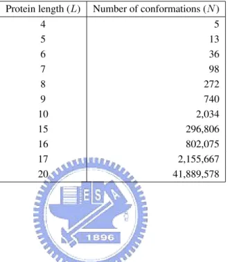
with respect to different number of nodes. It is performed on an 8-processors PC-based Linux cluster system. . . 43 3.3 The number of conformations of proteins with the length of L residues in a

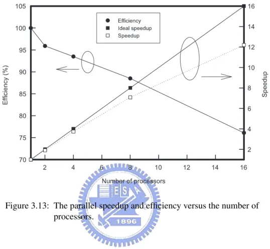
2D square lattice model. . . 49 3.4 The achieved parallel speedup and efficiency of the parallel computing

al-gorithm, where the tested case is a 17-mer with only hydrophobic residues. 53 4.1 A comparison list of the achieved results with respect to the two different

extractions. The target specification is adopted from realistic fabricated and measured data. . . 88

4.2 A list of process recipe and device parameters for the device optimization w/ and w/o considering the fluctuation reduction. . . 90 5.1 Eight different random number generation schemes and their expressions. . 114 5.2 List of the root-mean-square (RMS) errors of the extracted results

com-pared with the measured data for the four N-MOSFET devices. The device dimension is in µm. The oxide thickness of target devices are 3.36nm and the working temperature is settled at 298.15K. The chaotic random number generator is used in this simulation. . . 115 6.1 List of the residual of squares in the six response surface models. . . 140 6.2 List of the range of designing parameters and the optimized parameters for

the current mirror amplifier circuit. . . 144 6.3 List of the specified targets and the extracted results for the current mirror

1.1 Illustration of a basic flow in the field of electronic design. . . 3

1.2 The basic contents of the proposed UOF. . . 5

2.1 The values of f (x1, x2) respect to different x1 and x2 values. . . 11

3.1 An illustration of the architecture of UOF. Solid lines indicate inheritance and dashed lines indicate the ownership. . . 14

3.2 The class hierarchy of the UOFProblem and UOFSolver. The solid lines indicate inheritance. . . 14

3.3 The working flow and object inner connections in UOF from users’ point of view. . . 22

3.4 The working flow of GetResult in TCADProblem. . . 25

3.5 The flowchart of TCADEvaluator. . . 26

3.6 The basic working flow of the developed parallelization approach. . . 33

3.7 The constructed 32-node PC-based cluster. . . 34 xvii

3.8 An illustration of the cross-section view for the n-type double-gate MOS-FET device. . . 37 3.9 Adaptive finite volume solution algorithm for each decoupled

semiconduc-tor device equation. A is the system matrix, Z is the unknown vecsemiconduc-tor, and F is the nonlinear vector. . . 38 3.10 Parallel domain decomposition for the two-dimensional double-gate

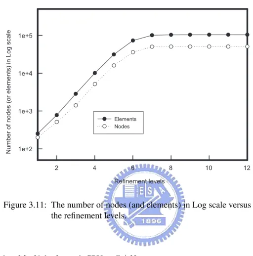
MOS-FET. The dash-lines indicate the boundary of partition domains. . . 39 3.11 The number of nodes (and elements) in Log scale versus the refinement

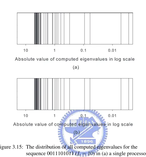
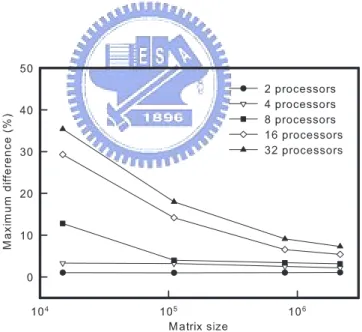
levels. . . 42 3.12 The maximum difference versus the number of nodes. . . 44 3.13 The parallel speedup and efficiency versus the number of processors. . . . 45 3.14 A computational flowchart of the implemented parallel method. . . 52 3.15 The distribution of all computed eigenvalues for the sequence 0011101011

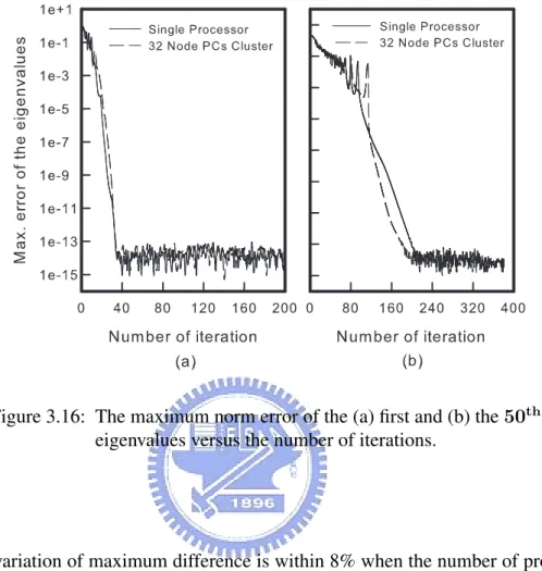
(L = 10) in (a) a single processor (b) and 32-node PC-based Linux cluster. . 54 3.16 The maximum norm error of the (a) first and (b) the 50th _eigenvalues

ver-sus the number of iterations. . . 55 3.17 The eigenvalues of the transition matrix of a 17-mer with only hydrophobic

residues. The dimension of the transition matrix is 2155667 by 2155667, and 50 eigenvalues have been computed. . . 56

3.18 The achieved load balancing versus the number of processors for the tested case of a 17-mer with only hydrophobic residues. . . 56 3.19 The achieved parallel efficiency versus the matrix size for different number

of processors. . . 57 3.20 The achieved load balancing versus the matrix size for different number of

processors. . . 57 3.21 (a) Visi’s logo and (b) its layout, where four tabbed pages, Property,

Dis-play, Color, and Info. are designed in Control panel. . . 61 3.22 An architecture of the developed classes in Visi. . . 61 3.23 Filter functionalities of Visi and the corresponding implementation classes. 62 3.24 The procedure flow for manipulating Visi to visualize a source data, and

the corresponding working flow in QVTKFrame. . . 64 3.25 Flowcharts for VTK data pipeline, and the list of derived classes for each

base class which marked with dash-line. . . 65 3.26 Flowcharts for the developed Visi data pipeline, and the list of derived

classes for CBaseActor class. The base class is marked with dash-line, while the function routines are marked with dot-line. . . 67 3.27 The tertiary structure of a catalytic antibody. (a) The structure data without

3.28 (a) The potential profile for a 2D MOSFET device, and (b) the zoom-in plot in the channel region of MOSFET device with contour lines and scalar bar. . . 69 3.29 The carpet plot for 2D potential profile by applying Warp-Scalar filter with

different color mapping schemes. . . 70 3.30 (a) The surface potential plot of a 3D MOSFET device. (b) The transparent

plot for potential profile and discrete implant doping atoms. . . 70 3.31 (a) X-Y and (b) X-Z cut planes of 3D MOSFET potential profile. . . 72 3.32 The carpet plots for (a) X-Y and (b) X-Z cut planes. . . 72 4.1 A working flow of the implement methodology for the reverse modeling

problem in tuning fabrication parameters. . . 81 4.2 An illustration of the target I-V curves to be extracted and empirical

knowl-edge. The important sections are pointed out in circles. The inset plot is a cross-section view of the simulated MOSFET with LDD doping profile. . . 85 4.3 An illustration of the initial doping profile for the explored 65 nm

N-MOSFET. . . 88 4.4 The optimized 65 nm N-MOSFET doping pro le for the device (a) without

4.5 The optimized doping profiles from the channel surface deep into the sub-strate. The 1-section is located at the center of device channel (x = 0). . . . 92 4.6 Doping profile from the source to drain along the channel direction 2 nm

below the interface between the gate oxide and the silicon substrate. The inset of the figure shows the structure of the optimized 65 nm N-MOSFET. 93 4.7 Plots of band profile for the optimization with and without considering the

threshold voltage fluctuation under the on-state; (a) is from the surface to the substrate and (b) is along the channel direction from the source to the drain which is about 2 nm below the channel surface. . . 94 4.8 Plots of band profile for the optimization with and without considering the

threshold voltage fluctuation under the off-state; (a) is from the surface to the substrate and (b) is along the channel direction from the source to the drain which is about 2 nm below the channel surface. . . 95 4.9 The achieved accuracy of the extracted I-V curves for the explored 65 nm

N-MOSFET. . . 96 4.10 The performance comparisons among three different evolutionary

strate-gies. There are totally 31 process and device parameters to be optimized in the case of the 2D process and device simulations. The total time is about 70 hours on a PC-based Linux cluster with 16 processors. . . 97

5.1 An illustration of the equivalent circuit model in connecting the device fab-rication and circuit design. . . 100 5.2 An illustration of the proposed hybrid intelligent computational methodology.102 5.3 The sensitivities examination of the parameters to be extracted in the

com-pact model. . . 106 5.4 The BSIM-4 extracted (solid-line) and measured (dot-lines) IDS− VDSand

IDS− VGScurves of the 90 nm MOSFET (width = 10.0 µm), where VBS = 0 V and VGSvaries from 0.4 to 1.4 V, and VDS = 0.1 V and VBS varies is 0 to -1.5 V. . . 107 5.5 The EKV extracted (solid-line) and measured (dot-lines) IDS − VDS and

IDS − VGS curves are of the 0.18 µm MOSFET, where VBS = -0.6V and,

VGS migrates from 0.4 to 1.4 V, and VDS = 1.3V and VBS migrates is 0 to -0.9 V. . . 108 5.6 (a) the score convergence of different extraction methods, and (b)the score

convergence behavior w/ and w/o applying NN as a director during the evolutionary process, where the testing is with BSIM-4 model applying to four 0.13 µm MOSFETs. . . 110 5.7 The score convergence behavior of our proposed method and pure GA for

5.8 The BSIM4-model extracted (solid-line) and measured (dot-lines) (a) IDS -VDS and (b) IDS-VGS curves of the MOSFET, where length = 90nm and width = 10µm. We notice that the chaotic random number generator is used in this simulation. . . 115 5.9 Comparison of the convergence score in GA with different random number

generation schemes. In this extraction experiment, GA extracts a single N-MOSFET device. . . 116 5.10 Comparison of the convergence score in GA with different random number

generation schemes. In this extraction experiment, GA extracts four N-MOSFET devices at the same time. . . 117 6.1 Functional blocks for the proposed simulation-based hybrid optimization

approach. . . 122 6.2 The optimization flow for the hybrid optimization approach. . . 123 6.3 The explored current mirror amplifier circuit. The transistors MB and MS

provide the current source for the differential amplifier. The transistors M1 and M2 form the differential amplifier, and transistors M3∼M6 make up the current mirror. . . 126 6.4 (a) The residual normal probability plot and (b) the residuals vs. predicted

6.5 (a) The residual normal probability plot and (b) the residuals vs. predicted plot for the response 1.0/Sqrt(F T ). . . 142

6.6 (a) The residual normal probability plot and (b) the residuals vs. predicted plot for the response P M1.57_{. . . . 143}

6.7 (a) The residual normal probability plot and (b) the residuals vs. predicted plot for the response CMRR−2.34_{. . . 144}

6.8 (a) The residual normal probability plot and (b) the residuals vs. predicted plot for the response Sqrt(SR+). . . 145

6.9 (a) The residual normal probability plot and (b) the residuals vs. predicted plot for the response 1.0/Sqrt(SR−). . . 146

6.10 Scatter plot calculated from the response surface model versus values ob-tained from circuit simulator for (a) GAIN and (b) 1.0/Sqrt(F T ). . . 147

6.11 Scatter plot calculated from the response surface model versus values ob-tained from circuit simulator for (a) P M1.57_{and (b) CMRR}−2.34_{. . . 148}

6.12 Scatter plot calculated from the response surface model versus values ob-tained from circuit simulator for (a) Sqrt(SR+) and (b) 1.0/Sqrt(SR−). 149

7.1 An illustration of the problem domain and boundary conditions in the ex-amined antenna. The problem domain is surrounded by the edges a, b, c and d; and all edges satisfy the third kind boundary conduction. The black rectangular frame near the upper line is the contact for input excitation. . . 156

7.2 The linear tetrahedral element. The labels for four nodes are local indices in FEM. . . 157

7.3 A flowchart for the proposed optimization approach in antenna design. In this procedure, after constructing the geometry of the new antenna, the corresponding input file for extern simulator is also generated and passed to the external simulator for further simulation and analysis. In this work, HFSS is applied as the external simulator to evaluate the performance of the new antenna. . . 159

7.4 The original geometry of examined antenna and the illustration of parti-tioned segments. The upper line presents the ground plane and the lower rectangle behaves as the radiation element. The black rectangular frame near the upper line is the contact for input excitation. The partitioned seg-ments allow us to perturb the geometry without spatial limitation in a spe-cific region. . . 165

7.5 The return loss (S11) of the original geometry. The antenna is a dual-band design but has only one clear dual-band at 2.6GHz. The return loss on the frequency 5 GHz still has room for improvement. . . 166

7.6 An optimized geometry of the examined antenna after our optimization scheme. The geometry of radiation element is obviously tuned by GA to enhance the transmitting and receiving properties of the antenna. . . 167

7.7 The return loss (S11) of the optimized geometry. One can find that the return losses corresponding to dual operating frequencies are less than 20 dB after the proposed optimization scheme. . . 168

7.8 The gain pattern for the original antenna at 2.6GHz. The left object is the 3D gain pattern. The right one is the 2D gain pattern. The solid line presents the gain pattern in the xz-plane, and the dashed line is the gain pattern in the xy-plane. . . 169

7.9 The gain pattern for the original antenna at 4.9GHz. The left object is the 3D gain pattern. The right one is the 2D gain pattern. The solid line presents the gain pattern in the xz-plane, and the dashed line is the gain pattern in the xy-plane. . . 170

7.10 The gain pattern for the optimized antenna at 2.6GHz. The left object is the 3D gain pattern. The right one is the 2D gain pattern. The solid line presents the gain pattern in the xz-plane, and the dashed line is the gain pattern in the xy-plane. . . 171 7.11 The gain pattern for the optimized antenna at 4.9GHz. The left object is

the 3D gain pattern. The right one is the 2D gain pattern. The solid line presents the gain pattern in the xz-plane, and the dashed line is the gain pattern in the xy-plane. . . 172 7.12 The fitness score versus the number of generations in the examination. The

mutation rate in this examination is 0.01 and single-point cut crossover scheme is adopted. The proposed optimization scheme enhances the an-tenna property within ten generations in this examination. . . 173 8.1 The source code could be downloaded from http://140.113.87.143/ymlab/uof/

Introduction

1.1 Motivation

The modern microelectronics industry involves many optimization jobs that are subject to simulated results from certain simulators, such as device model parameter extraction [1–3], automatic design of integrated circuit (IC) [4], process simulation [5], reverse modeling [6] and antenna optimization [7, 11]. These terms need to feed specific parameters into some commercial simulators to obtain the corresponding simulated results. The engineers adjust the parameters according to the results, and again feed the adjusted parameters to retrieve the improved results. This circular procedure continues until the results match the requirements of the customers or supervisors. Currently, this routine work is typically performed by engineers with expertise. Therefore, a well-defined framework can assist

engineers to complete their design works more easily with various optimization techniques. A major obstacle to designing a general-purpose optimizer in programming language is the difficulty in defining a comprehensive interface for problems and solvers. Appro-priate interfaces for problems and solvers produce objects that are heuristically easy to reuse again in a specific framework. Several optimization frameworks, such as GALIB [8], DESMO [9] and NP-Opt [10], have been proposed in the public domain. These packages have certain advantages, but still have room for improvement in terms of the connections between problem and solver for real-world applications, in particularly for the problems of electronic design.

1.2 Objectives

This dissertation implements a C++ unified optimization framework (UOF) for general problems and solvers. Based on the C++ design pattern techniques, the UOF enables users to define the problems and solvers from the fundamental level. The developed UOF is composed of two parts, the problem part and the solver part. The basic interface of problem-related classes contain initialization, evaluation and constraint procedures. The solver-related classes include the solver, solution, termination and information procedures. Separating each part into several classes increases the efficiency of reutilization. With-out considering the mathematical convergence property, one hybrid intelligent technique

for electronic design automation is also proposed and implemented in the UOF. In the proposed hybrid approach, an evolutionary method, such as genetic algorithm (GA), firstly searches the entire problem space to get a set of roughly estimated solutions. The numerical method, such as Levenberg-Marquardt (LM) method, then performs a local optima search and sets the local optima as the suggested values for the GA to perform further optimiza-tions. Several applications are presented to demonstrate the flexibility and extensibility of UOF.

Macro

Device Circuit System

Quantum mechanical Semiclassical Monte Carlo Drift-diffusion Relaxation -time approx Device M C R T A D D Circuit E le c tr ic a l B e h a v io r a l Logic

Timing Switch Gate RTL

F u n c tio n a l S tr u c tu r a l B e h a v io ra l Micro a1 1 a2 2 3 a3 4 a4 b1 b2 b3 b4 5 6 7 8 Vcc1 0 GND 0 a1 1 a2 2 3 a3 4 a4 b1 b2 b3 b4 5 6 7 8 Vcc1 0 GND 0 TCAD (Technology CAD) ECAD (Electronic CAD)

Figure 1.1: Illustration of a basic flow in the field of electronic design.

Figure 1.1 illustrates a basic flow of the electronic design. Toward the end of mi-croelectronics industry, it is related to semiconductor device manufacturing and assisted by technology computer-aided design (CAD) tools. The major topic in the macroscopic side is

the circuits design with the electronic CAD tools. The device compact models bridge these two areas, and the parameter extraction is the main problem in this part. These electronic design problems are very complicated and not always guaranteed to have an optimal solu-tion. Therefore, the designers or engineers only need to find one suitable solution which can meet all specifications. The purpose of the UOF is to integrate the hybrid approach with various CAD tools and empirical knowledge to assist the designers or engineers in searching the solutions that can match their specified targets.

The applications from the micro side to macro side which include the reverse doping profile problems, device model parameter extraction, integrated circuit design and the an-tenna design optimization, as shown in Fig. 1.2, are implemented with the UOF. Now the UOF can directly link to the following CAD tools, ISE TCAD tool, HSPICE and HFSS. The ISE TCAD tool provides a series of process and device simulators for the semicon-ductor devices. HSPICE is a well-known circuits simulator for ICs design. HFSS is the industry-standard software for 3D electromagnetic field simulation of high-frequency and high-speed components. Most electronic design problems are time-consuming tasks, and one parallel environment is established for the UOF to speedup the optimization procedure. Several applications are implemented with the proposed parallel technique to illustrate the developed environment. Furthermore, one open-source project, Visi is also implemented for high-dimensional engineering and scientific data visualization.

Applications Inverse Doping Profile Problem Parameter Extraction ICs Design Antenna Shape Optimization

Unified Optimization Framework - Protein Folding Dynamics

Problem

- Semiconductor Device Simulation

- Compact Model Parameter Extraction

An Open-Source Project 'Visi' for Scientific Visualization

Parallel Computing _{Visualization}Scientific Electromagnetics Circuit

Simulation Device

Simulation

Figure 1.2: The basic contents of the proposed UOF.

1.3 Outline

This dissertation is organized as follows. The review of conventional optimization frame-works are given in chapter 2. Chapter 3 then introduces the architecture of the UOF. It explains the detailed coding methodologies for the problem and solver, and provides pseudocode for building problems and solvers. The architecture of the developed paral-lelization technique and one open-source project for scientific visualization are also pre-sented. Chapters 4-7 present the applications of the UOF in the modern microelectronics industry, including 65nm CMOS device fabrication, VLSI device model parameter extrac-tion, VLSI circuit design problem and communication system antenna design problem, respectively. Conclusions are finally drawn in Chapter 8, along with recommendations for future research.

The Conventional Optimization

Framework

S

everal optimization frameworks, such as GALIB, DESMO and NP-Opt, have been proposed in the public domain. GAlib contains a set of C++ genetic algorithm ob-jects, which was developed at MIT. DESMO is a framework for “Discrete Event Simula-tion and MOdeling” developed at the University of Hamburg. NP-Opt is an object-oriented framework for optimization based on evolutionary computation techniques. These pack-ages have certain advantpack-ages, but still have room for improvement in terms of the connec-tions between problem and solver for real-world applicaconnec-tions.

2.1 GALIB

GAlib [8] contains a set of C++ genetic algorithm objects, which was developed at MIT. This library includes tools for using genetic algorithms to do optimization in any C++ pro-gram using any representation and genetic operators. The propro-gramming interface for the library includes general library information, genetic algorithm, population, scaling, selec-tion, genomes, and data structures. The users must define the representaselec-tion, genetic oper-ators and objective function for the problem when using GAlib, and users work primarily with two classes: a genome and a genetic algorithm. Each genome instance represents a single solution to the problem. The genetic algorithm object defines how the evolution should take place. The genetic algorithm uses the defined objective function to determine the fitness of each genome. It uses the genome operators and selection/replacement strate-gies to generate new individuals.

The GAlib is a well-known library for genetic algorithm, and provides basic compo-nents for users to define and solve their problems. However, the main drawback of GAlib is that it focuses on GA only and does not support other numerical or evolutionary opti-mization methods.

2.2 DESMO

A framework for Discrete Event Simulation and MOdeling (DESMO) [9] was developed at the University of Hamburg in the late 1980s. It has been continuously evolved over the last decade. Starting with Modula-2, the framework was ported to various programming languages including Smalltalk and C++. The latest version is DESMO-J which is based on a fully object oriented architecture and is completely implemented in Java. It presented bridges the gap between three different research areas: discrete event simulation, heuristic optimization methods and distributed systems technology. It bases on genetic algorithm to perform optimization works, and the fitness function comes from discrete event simulation. Since DESMO-J is a Java program, features of Java also apply to DESMO-J, and the Java’s Remote Method Invocation (RMI) is employed for distributed simulation optimization.

2.3 NP-Opt

NP-Opt [10] is an object-oriented framework for optimization based on evolutionary com-putation techniques to address NP-hard problems. The purpose of NP-Opt is to provide a high code reutilization for general optimization works. Three different methods: genetic algorithm, memetic algorithm and multiple start are built in the NP-Opt. The framework

also includes some refinements like population structure, fuzzy controlling of the evolu-tionary parameters and multiple populations. Five different types of recombination have been included so far, as well as two local search procedures. The class ”Framework” is the main control class of the NP-Opt framework. It provides all the possible control options to the user, such as problem type selection, instance to solve, method selection and execu-tion parameters. It also defines all the variables used to control and run each problem or method, and includes the calling procedures to the classes linked to it. All code of NP-Opt was developed in Java, and it also provides a graphical user interface for users. To gener-ate new problems in the NP-Opt, users must define the following: a representation for the problem, the method to evaluate a solution, the mutation scheme, the crossover operator, and the representation for the instance.

Many conventional optimization frameworks are based on evolutionary computation methods, and some even focus on genetic algorithm only. It is useful to develop opti-mization framework to include not only global evolutionary algorithms but also numerical deterministic methods. For more flexibility, it should allow user to mix different optimiza-tion methods for hybrid optimizaoptimiza-tion procedures. It is also beneficial for user to easily define their problems and to build new optimization solvers by themselves.

Compared with these frameworks, the developed UOF contains not only evolutionary algorithms but also numerical deterministic methods. Furthermore, the hybrid approach

which integrates both evolutionary and numerical algorithms is also can be easily imple-mented in the UOF. We use one minimization problem to compare the efficiency of the hybrid approach with the pure evolutionary or numerical algorithms. Consider a minimiza-tion problem in the following expression,

f (x1, x2) = 21.5 + x1sin(4πx1) + x2sin(20πx2), (2.1)

where −3.5 ≤ x1 ≤ 12.1 and 4.1 ≤ x2 ≤ 5.8. Figure 2.1 shows the values of f (x1, x2)

respect to different x1 and x2. The minimal value of f function is 3.8532 and occurs at

(x1, x2) = (11.8759, 5.7745).

Table 3.3 shows the found solutions by different methods. According to the results, the numerical method can not find the global minimal value without a good initial guess. The proposed hybrid approach can quickly get the optimal solution, and the evolutionary approach can also find a good solution, but it requires much longer time for iterations. The hybrid approach demonstrate excellent efficiency in solving this minimization problem.

0 5 10 4.5 5 5.5 0 10 20 30 0 5 10 0 10 20 30 x1 x2 f(x1,x2)

Figure 2.1: The values of f (x1, x2) respect to different x1and x2

values.

Table 2.1: The found solutions of different methods in solving the minimization problem of Eq. 2.1.

# of iterations Numerical method GA The hybrid approach

1 11.54 11.54 11.54 10 9.48 10.99 10.850 20 8.72 9.946 7.603 40 8.72 8.054 5.344 60 8.72 5.984 3.853 100 8.72 4.015 –

The Unified Optimization Framework

The UOF is an object-oriented framework for general problem optimization. Based on biological inspired techniques, numerical deterministic methods, and C++ objective design, the UOF [34] itself has significant potential to perform optimization operations on various problems. The components of the UOF can be separated into problem and solver parts. The details of these two components and the architecture of the UOF are presented in this chapter. Several implementation examples are given to demonstrate the way to construct solvers or problems in the UOF. Furthermore, one developed parallelization technique are illustrated through some applications. One open-source project, Visi for high-dimensional engineering and scientific data visualization is also presented at the end of this chapter.

3.1 The Architecture of the UOF

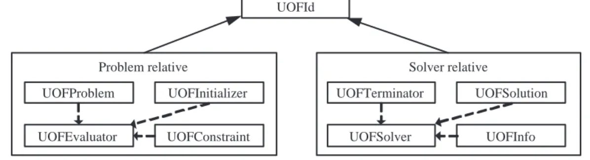
Figure 3.1 illustrates the class diagram of UOF. The class UOFId is the base-class of every class here for run-time type information (RTTI) purposes. All members in UOF can be easily categorized into problem-related and solver-related classes. The UOFProblem class is the main class to define the problem; the UOFInitializer class is responsible for the ini-tialization of the solution for each problem; the UOFEvaluator class provides the method for evaluating the result obtained by the UOFProblem derived classes; the UOFConstraint class defines the constraint of each parameter; the UOFSolver class takes the major charac-ter in solver relative category; the UOFSolution class stores possible solutions and several operators of the specified solver; the UOFTerminator class judges when and how to stop the optimization process of the solver, and the UOFInfo class logs the behavior of the solver during the solving process. All classes in both categories are abstract classes, and need to be implemented in derived classes.

Figure 3.2 shows the built-in class specializations of the most important two classes in current UOF. As shown in Fig. 3.2a, NPProblem, FunctionProblem, and ExtSimProblem are directly inherited from UOFProblem. The UOFProblem class has general interfaces for the user to define any problems. NPProblem provides convenient interfaces for defining NP-hard problems such as TSP and the single/parallel machine scheduling problem. More-over, optimization problems of linear and non-linear continuous functions, such as DeJong

UOFProblem UOFConstraint UOFEvaluator UOFInitializer UOFSolution UOFInfo UOFSolver UOFTerminator

Problem relative Solver relative

UOFId

Figure 3.1: An illustration of the architecture of UOF. Solid lines indicate inheritance and dashed lines indicate the ownership.

functions [12], can be defined by FunctionProblem class. ExtSimProblem class has ba-sic linkages to external software to perform simulations, such as commercial TCADs and ECADs. The solver-related classes illustrated in Fig. 3.2b can be separated into two cate-gories, namely gradient-based and the population-based solvers. The fundamental abstract classes are described in detail in the following sections.

(a) (b)

UOFSolver UOFProblem

FunctionProblem NPProblem ExtSimProblem

SPICE TCAD ECAD

LMSolver

BFGSSolver PopBaseSolver

ACOSolver PSOSolver GABaseSolver

Figure 3.2: The class hierarchy of the UOFProblem and UOFSolver. The solid lines indicate inheritance.

3.1.1 The UOFProblem Class

The interface of UOFProblem class is defined as follows:

class UOFProblem : public UOFId

{

public:

virtual double GetResult(void *inp)=0;

virtual void GetResult(void *inp,void *out)=0;

virtual void GetJacobianResult(void *inp,void *out)=0; virtual void GetExternalData(void *data)=0;

virtual void SetConstraint(void *cnt)=0;

}

The GetResult function is the major function of UOFProblem class to calculate the results of given parameters. The function has two overloaded versions. One is a convenient version which returns a result in a ‘double’ format, and the other is the type-free version that returns data in any specified type. The GetJacobianResult function is used by the gradient-based solvers, which return the Jacobian matrix back to the solver.

3.1.2 The UOFEvaluator Class

The UOFEvaluator interface is declared as follows:

class UOFEvaluator : public UOFId

{

public:

UOFEvaluator(UOFProblem & src) : m pProblem(& src){} virtual double operator()(void* src) = 0;

UOFProblem *m pProblem;

}

The UOFEvaluator itself is a function object [21] that acts like a function pointer in C, but takes advantages of C++ object-oriented programming. It stores the pointer of UOF-Problem, and performs the communications with UOFProblem in the operator() function. UOFEvaluator is like an agent that connects the UOFProblem and UOFSolver to reduce the coupling effects between UOFProblem and UOFSolver.

3.1.3 The UOFInitializer Class

The interface of UOFInitializer:

class UOFInitializer

{

public:

virtual void operator()(void* src, UOFProblem* pT);

}

UOFInitializer performs solution initialization, which is called by UOFSolution object. The solution to be initialized should be transferred to void* type. Moreover, UOFInitializer also stores the UOFProblem pointer, and allows the user to retrieve extra information in UOFProblem object.

3.1.4 The UOFSolver Class

The interface of UOFSolver is defined as follows: class UOFSolver : public UOFId

{

public:

virtual void Initialization()=0; virtual void Solve()=0;

}

In this class, the Initialization function performs the initialization steps before the solving procedure. Configuration function allows the user to configure the solver through a script file, and the Solve function controls the entire optimization process.

The solvers of the UOF comprises two parts, the gradient-based and the population-based solver. The gradient-population-based solver includes the Broyden-Fletcher-Goldfarb-Shanno (BFGS) [13] and Levenberg-Marquardt (LM) methods [14]. Both of these are quasi-Newton methods and are popularly used in deterministic solving packages [15]. The population-based solver includes several heuristic methods such as genetic algorithm (GA) [16], particle swarm optimization (PSO) [17], ant colony optimization (ACO) [18] and simulated annealing method [19, 20].

In 1970, an alternative update formula was suggested independently by Broyden, Fletcher, Goldfarb, and Shanno. The method is now called the BFGS algorithm [13]. The BFGS method is derived from the Newton’s method and is used to solve unconstrained nonlin-ear optimization problems. The LM method is a quasi-Newton method to accelerate the Gauss-Newton method. The Gauss-Newton method is the basic algorithm for solving the nonlinear optimization problem. Due to the nonlinear property of the problem, a gradient for each variable can be obtained. It starts from an initial guess, and follows the direction

of the normal of the gradient to find the optimal solution. Therefore, the initial guess must be chosen carefully, or the solution may fell into a local optima. Unlike the Gauss-Newton method has the fixed steps toward the solution, LM optimization method detects that some regions with monotonic variation property can be speed up by increasing the step size. On the other hand, when the optimization process encounters a sensitive region, the step should be shorten to avoid skipping the optimum.

GA is a global search optimization method based on the mechanics of natural selec-tion and natural genetics. It works with a coded of parameters string called chromosome instead of the solutions themselves. Each chromosome represents a solution set, and the fitness functions used to measure the survival scores of all chromosomes in the popula-tion. Then the GA will accord its selection scheme to select several chromosomes for copulation, discard unwanted chromosomes, and adopt the crossover scheme to produce the new generation. Then the GA will apply fitness function for the new population again and loop this cycle until certain stop criteria is achieved. The GA includes following parts, the problem definition, the gene encoding, fitness evaluation, selection, crossover, muta-tion. Particle swarm optimization is a population based stochastic optimization technique developed by Eberhart and Kennedy in 1995, inspired by social behavior of bird flock-ing or fish schoolflock-ing. The system is initialized with a population of random solutions

and searches for optima by updating generations. However, unlike GA, PSO has no evo-lution operators such as crossover and mutation. In PSO, the potential soevo-lutions, called particles, fly through the problem space by following the current optimum particles. The particle swarm optimization concept consists of, at each time step, changing the velocity of (accelerating) each particle toward its pbest and lbest locations (local version of PSO). Acceleration is weighted by a random term, with separate random numbers being gener-ated for acceleration toward pbest and lbest locations. The ant colony optimization is also a population-based approach to the solution of combinatorial optimization problems. The basic ACO idea is that a large number of simple artificial agents are able to build good so-lutions to hard combinatorial optimization problems via low-level based communications. Annealing process is the way in which a metal cools and freezes into a minimum energy crystalline structure (the annealing process) which was proposed by Nicholas Metropolis in 1953. In 1985, Kirkpatrik proposed the simulated annealing (SA) optimization method which mimics the real annealing process in the system to find a optimal cooling process to get the minimal energy crystalline structure (optimal solution). First, they use SA to solve discrete problems such as T.S.P, Backpacking Problem, N.P. completeness problems, and so no. Recently, SA is widely used in: layout routing, parameters extraction ... etc.

3.1.5 The UOFSolution Class

UOFSolution is an abstract class to describe the solution format used in any UOF compo-nents. The class declaration is listed as below:

class UOFSolution : public UOFId

{

public:

UOFSolution(UOFInitializer *init, UOFEvaluator *eval); UOFSolution(const UOFSolution&);

UOFSolution& operator=(const UOFSolution&); virtual UOFSolution* clone() const;

virtual void copy(const UOFSolution&); virtual double score();

}

The score function in UOFSolution invokes UOFEvaluator to obtain the simulation re-sults of given parameters, and calculates the fitness score.

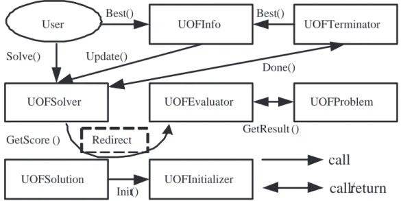
User UOFSolver UOFSolution UOFEvaluator UOFInitializer UOFProblem UOFInfo UOFTerminator Solve() GetScore () Done() Redirect Init() GetResult () Update() Best() Best()

call

call/return

Figure 3.3: The working flow and object inner connections in UOF from users’ point of view.

3.1.6 The Working Flow of the UOF

Figure 3.3 shows the working flow and object inner connections in the UOF from the user point of view. Users initially call the Solve function in the UOFSolver class to start the op-timization operation. Meanwhile, the UOFInitializer initializes the UOFSolution objects. The Solve function invokes the GetScore function in UOFSolution class to calculate the re-sults from the given parameters. The UOFSolution class redirects and passes the GetScore message to the UOFEvaluator class. The UOFEvaluator object passes the solution to UOF-Problem, and calls GetResult to obtain the corresponding results. While the solver solves the problem, in each iteration the UOFInfo updates the current status of the solver, such as

the best parameter set. Moreover, the UOFTeriminator also updates the current best solu-tion from UOFInfo, and tells UOFSolver when to stop the optimizasolu-tion procedure. Finally, users can obtain the best solution from the UOFInfo object.

3.2 Implementation Examples

To apply the UOF with any specific problem, we first convert the problem as an optimiza-tion problem. The adjustable parameters, the evaluaoptimiza-tion criteria and the targets should be defined clearly. In the next step is to build the problem class for the specific problem. It is an easy way to duplicate one default problem class and alter the related variables and functions in the class accordingly. This section constructs of simulation-based problems and two solvers step by step given to demonstrate the capability and extensibility of UOF.

3.2.1 Simulation-based Problem

The major task in implementing a simulation-based problem in UOF is to encapsulate the I/O operations to external simulators within the subclass of the UOFProblem class. This section describes the specialization of UOFProblem class without loss of generality, tak-ing the TCAD reverse modeltak-ing problem as an example. Three classes, TCADProblem, TCADEvaluator and TCADInitializer, are derived. TCADInitializer is responsible for gen-erating a random initial parameter set. TCADEvaluator measures the error between the

target data and the simulated result. TCADProblem provides the GetResult, GenerateIn-termediateFiles, and ReadOutputFiles functions. Figure 3.4 shows the working flow of these methods. The Figure indicates that the GetResult function is rather simple. GetRe-sult first calls the GenerateIntermediateFiles function to generate the input files required by the simulator, then runs the simulator, and finally calls the ReadOutputFiles to retrieve the simulated result. GenerateIntermediateFiles function generates the input files required by the simulator. These files are called m InterMediateFiles. This procedure requires the m InputFile data, and maps the value of each parameter into the m InputFile to generate the m InterMediateFiles. The ReadOutputFiles function parses the output file of the simulator to retrieve the necessary simulated result. Figure 3.5 shows the flowchart of TCADEvalua-tor. TCADEvaluator calls GetResult in TCADProblem to retrieve the simulated result, and returns the error between the simulated result and the target data to the caller.

3.2.2 Genetic Algorithm Solver

This subsection describes the construction of a genetic algorithm solver. The first step is to declare three classes named GABaseSolver, TerminateUponIteration and GA1DArraySolution, which are inherited from PopBaseSolver, UOFTerminator and PopSolution, respectively. In this experiment, the stopping criteria was set to reach the maximum iteration, therefore, so the TerminateUponIteration function would return true if the maximum iteration was

GetResult GenerateIntermediateFiles ReadOutputFiles Output File TCAD Simulator Input File Parameters

Simulator-output File Parser

Intermediate File

Simulated Result

Figure 3.4: The working flow of GetResult in TCADProblem.

reached. The GA1DArraySolution class rewrites the GetScore function, and declares the GA crossover and mutation operator. The Solve function is the entry point of the solver called by the main function of the program. It first calls the Initialization, then performs Evolve to evaluate each individual and perform further genetic operators, namely selection, crossover, and mutation until TerminateUponIteration (in Done function) reports the “true” event. The pseudocode for Solve and Evolve functions are as follows.

TCADProblem

TCADEvaluator

GetResult

Parameters

Simulated Result Parameters

Measure

Error

Measured

Data

Score

Figure 3.5: The flowchart of TCADEvaluator.

{ Initialization(); do{ Evolve(); }while(!Done()); } void GABaseSolver::Evolve() {

1.Compute fitness score of each parameter set For each solution (in m Pop array):

Call m Pop[a]→ score(); 2.Sort the fitness score:

sort(m Pop.begin(),m Pop.end(),MinScore); 3.Selection operation:

(*m pSlct)(m Pop, selected); 4.Crossover operation:

(*m pCros)(selected[p1], selected[p2], m Pop[a], m Pop[b]); 5.Mutation operation:

(*m pMutr)(m Pop[a]);

}

3.2.3 Particle Swarm Optimization Solver

The PSO, like the GA, is a population-based solver, meaning that the content are alike. The major difference between these two solvers occurs in the Evolve function. The PSOSolver performs a move operation defined in the PSOMove function of the PSO1DArraySolution

to update the parameters after sorting the individuals. The pseudocode of the Evolve func-tion is given below.

void GABaseSolver::Evolve()

{

1.Compute fitness score of each parameter set For each solution (in m Pop array):

Call m Pop[a]→ score(); 2.Sort the fitness score:

sort(m Pop.begin(),m Pop.end(),MinScore); 3. Move particles:

(*m pMove)(m Pop[0], m Pop[i], m Vc, m K1, m K2);

}

void PSOMove::operator()

( PopSolution* bestp, PopSolution* currentp, double w, double k1, double k2)

{

1.Convert bestp and currentp to PSO1DArraySolution type 2.Compute the velocity of currentp;

3.Update the position of currentp;

3.2.4 Basic Experiment on Traveling Salesman Problem

The TSP is a well-known discrete combinational problem. Its objective is to discover a minimized route for a salesman to visit each city only once and finally return to the starting point. Three classes, TSPProblem, TSPEvaluator, TSPInitializer, which are inherited from UOFProblem, UOFEvaluator, UOFInitializer, respectively, are defined to implement TSP in the UOF standard. The TSPInitializer is utilized to create a random string as a route to travel to each city. The TSPEvaluator simply returns the total length of the given route, which is derived from TSPProblem. Pseudocode for TSPInitializer, TSPEvaluator, and GetResult function in TSPProblem is given below.

class TSPInitializer : public UOFInitializer

{

public:

virtual void operator()(void* src, UOFProblem* pProblem)

{

1.Random generates the initial solution S 2.Set S to src

}

class TSPEval : public UOFEvaluator

{

public:

virtual double operator()(void* src)

{

1.Get total length of the route from TSPProblem: TotalLength = m pProblem → GetResult(src); 2.Return TotalLength

} }

double TSPProblem::GetResult(void* param)

{

1.Convert param into proper data type 2.Compute total distance from param 3.Return total distance

Table 3.1: The optimized result of the TSP.

Method Geometry # of cities Average # of Iteration Percent of success run

GA Circle 30 2231 80% ACO Circle 30 4 80% GA Circle 50 6562 30% ACO Circle 50 18 60% GA Matrix 9 24 100% ACO Matrix 9 4 100% GA Matrix 25 3600 30% ACO Matrix 25 26 100%

Four geometric distributions of cities were explored. The first and second distributions formed a circle, and contained 30 and 50 cities, respectively. The third and fourth distrib-utions were 3 × 3 and 5 × 5 matrices, respectively. The GA and ACO were performed to compare the efficiency of each problem. Table 3.1 summarizes the result, revealing that the ACO method is better than GA method for solving this problem. The result also confirms that the UOF can solve the discrete combinational optimization problem.

3.3 The Developed Parallelization Technique

It is known that many engineering problems are quite complicated and time-consuming jobs which require huge resource for computations. Therefore, a parallelization technique can reduce the computing time and benefit the design flow in the electronic design. Based

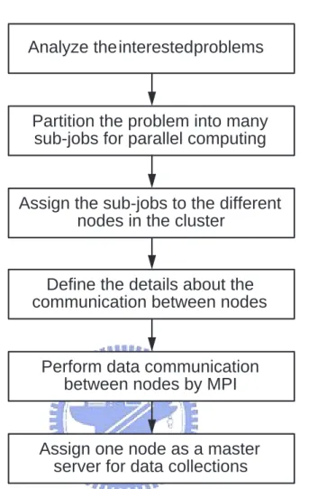
on the message passing interface (MPI) libraries and some partition techniques, we have developed one parallelization flow to speedup the simulation and optimization processes. Figure 3.6 shows a basic working flow of our parallelization approach. First we need to analyze the problems, try to partition the problem into sub-jobs, and then dispatch these sub-jobs to the processors in the cluster. Meanwhile, the data communications between processors should be carefully defined, and the communications are performed with the MPI libraries. Finally one processor in the cluster may be regard as the master sever to monitor and collect the necessary outputs in each processor of the PC-based Linux cluster. The benchmarks, such as speedup, efficiency, and maximum difference with respect to various numbers of processors can be adopted to evaluate the parallel performances. The speedup is the ratio of the code execution time on a single processor to that on multiple processors. The efficiency is defined as the speedup divided by the number of processors. In our PC-based Linux cluster, as shown in Fig. 3.7, each PC is equipped IBM eServer EM64T with 3.6 GHz CPU, 2 GB memory, and Intel 100 MBit fast Ethernet. All PCs in the constructed 32-nodes cluster system are connected with 100MBit 3Com Ethernet switch.

The major challenges in implementing parallelization are the way to partition the prob-lems into sub-jobs. It is entirely dependent on the probprob-lems, and will affect the performance of the parallelization. Conventionally, there are two different ways to perform the partition.

Analyze the interested problems

Partition the problem into many sub-jobs for parallel computing

Assign the sub-jobs to the different nodes in the cluster

Define the details about the communication between nodes

Perform data communication between nodes by MPI

Assign one node as a master server for data collections

Figure 3.6: The basic working flow of the developed parallelization approach.

One way is to partition the problem domain into sub-domains, and then perform the cal-culation or simulation on each sub-domain separately. For the parallelization of the semi-conductor device simulation [61], we use a domain decomposition approach to partition the simulation domain into sub-domains, and then simulate the sub-domains on different processors in the cluster. Another method is to perform parallelization based on the used

Figure 3.7: The constructed 32-node PC-based cluster.

algorithms. For example, according to the property of genetic algorithm, we can simply execute the GA on each processor simultaneously for the parallelization. In following, two applications of the developed parallelization method are presented to show the efficiency of the proposed method.

3.3.1 Parallelization for Nanoscale Double-Gate MOSFETs

Simula-tion

In this section, we introduce the parallelization for semiconductor devices simulation which is based on the partition of the simulation domain. In this investigation, based on a poste-riori error estimation, the triangular mesh generation, the adaptive finite volume method,

the monotone iterative method, and the parallel domain decomposition algorithm, a set of two-dimensional quantum correction hydrodynamic (HD) equations is solved numerically for the double-gate metal-oxide-semiconductor field effect transistors (MOSFETs) on our constructed cluster system.

Classical HD model consists of at least five coupled partial differential equations (PDEs). The HD equations in semiconductor device simulation are as follows,

4φ = q εs (n − p + D), (3.1) 1 q∇ · Jn= R(n, p), (3.2) 1 q∇ · Jp = −R(n, p), (3.3) ∇ · Sn = Jn· E − n( wn− w0 τnw(Tn) ), (3.4) ∇ · Sp = Jp· E − p( wp− w0 τpw(Tp) ), (3.5)

where φ is the electrostatic potential and n and p are classical electron and hole concen-trations. Tn and Tp are electron and hole temperature (K). The electric field E (V/cm) is defined by E = −∇φ, q is the elementary charge its unit is coulomb. εsis the semiconduc-tor permittivity (F/cm). w0 is the average carrier energy (eV) in the thermal equilibrium,

and the net doping concentration is D(x, y) = N+

D(x, y) − NA−(x, y). R is the net recom-bination rate (cm−3_s−1_{), and τ}

(s) approximations. The average carrier energy consists of the thermal energy and the drift energy wn= 3 2kBTn+ 1 2m ∗ nvn2, (3.6) wp = 3 2kBTn+ 1 2m ∗ pvp2, (3.7)

for electrons and holes, respectively. m∗

nand m∗pare the electron and hole effective masses (Kg). vn and vp are the electron and hole mean velocities (cm/s). The carrier’s currents and energy flux densities are given by

Jn= −qµnn∇φ + qDn∇n + µnkBn∇Tn, (3.8) Jp = −qµpp∇φ + qDp∇p + µpkBp∇Tp, (3.9) Sn = Jn −qwn+ Jn −qkBTn+ Qn, (3.10) Sp = Jp +qwp+ Jp +qkBTp+ Qp, (3.11)

where µn and µp are the carrier mobility (cm2_{/V−s). The diffusion coefficients, D}

n and

Dp (cm2/s), satisfy the Einstein relation. Qn and Qp are the heat flows. However, to simulate the nanoscale double-gate MOSFETs, the classical HD model is insufficient due to significant quantum confinement effects. Therefore, we have to consider the quantum mechanical effects in the classical HD model above. The quantum correction equation for the quantum corrected inversion-layer charge densities nQM is

nQM = a0nCL(1 − exp(−a1ξ2(1 − 1 2( ξ ξ0 )2_{) − a} 2ξ3), (3.12)

Gate Oxide 1

Gate 1

Gate Oxide 2

Gate 2

p type

Drain

Source

n

+

n

+ Leff Tsi Tox L L L

X

Y

Figure 3.8: An illustration of the cross-section view for the n-type double-gate MOSFET device.

where nCLis the classical electron density solved from the Poisson equation. ξ = x/λth is dimensionless and λth = ( ~2

2m0kBT)

1/2 _{is the thermal wavelength ( ˚A), ~ is the reduced}

Planck constant (J−s), m0 is the electron rest mass (Kg), kB is the Boltzmann constant (J/K), T is the absolute temperature (K) and ξ0 = Tsi/2λthis dimensionless. Together with the auxiliary equation (3.12), the conventional HD model forms a quantum correction HD model. The associated boundary condition for the model is the same with the conventional HD model.

We solve the above quantum correction HD model with a parallel adaptive computing technique for nanoscale double-gate MOSFETs, as shown in Fig. 3.8. The full set of quantum HD model is firstly decoupled with Gummel’s method, and each decoupled PDE is solved sequentially. Figure 3.9 shows the adaptive computational procedure. For each

Finite Volume Approximation Simulation Domain Discretization Post-process Error > TOL Mesh Refinement No Yes Each Semiconductor Device Equation Start Nonlinear System AZ = -F(Z) Monotone Iterative Solver

Figure 3.9: Adaptive finite volume solution algorithm for each

decoupled semiconductor device equation. A is the system matrix, Z is the unknown vector, and F is the nonlinear vector.

decoupled semiconductor device equation, we first partition the solution domain into a set of finite volumes. Each decoupled PDE is then approximated by the finite volume method. After the assembling the nonlinear algebraic system, the monotone iterative solver is directly applied to solve the system of nonlinear equations. Once an approximate solution is computed, a posteriori error analysis is performed to assess the quality of the approximate solution. The error analysis will produce error indicators and an error estimator. If the

Gate Oxide 1

Gate 1

Gate Oxide 2

Gate 2

Drain

Source

#n #n-1 CPU #1 #2 . . .

Figure 3.10: Parallel domain decomposition for the two-dimensional double-gate MOSFET. The dash-lines indicate the boundary of partition domains.

estimator is less than a preset error tolerance (TOL), the adaptive process will be terminated and the approximate solution can be post-processed for solving next equation or analyzing physical properties. Otherwise, a refinement scheme is employed to refine the current elements depending on the magnitude of the error indicator for that element. A newer partition of the domain is thus created and a new solution procedure is repeated.

In parallelization, a pre-processor will prepare the input data required for each client. In the configuration of MPI and Linux cluster, input data is prepared on the pre-processor and is sent to each client through TCP/IP, and then all clients do their own local jobs and exchange essential data with the neighbor clients. When each client completes its own jobs, it sends the results to a post-processor. The post-processor then estimates the solution er-ror. If the estimator is larger than a TOL, the post-processor delivers the computed results