Advanced Spatio-Temporal Radio Channel
Model-ing and Joint Statistical Property Analysis for
Mac-rocellular Urban and Suburban Environments
NSC 92-2219-E-009-029
PART I Spatio-temporal Radio Channel Measurement
and Modeling in Urban and Suburban
Macro-cells
PART II A Physical and a Physical-Statistical
Spa-tio-Temporal Radio Channel Model for
Macro-cellular Environments
Part III Antenna-Array Spacing on Outdoor MIMO
Capacity
PART I Spatio-temporal Radio Channel Measurement
and Modeling in Urban and Suburban
Macro-cells
Abstract
Extended measurement of spatio-temporal radio channel for macrocellular systems in urban and suburban areas was carried out using a wideband vector channel sounder. In the meas-urement, TOAs (Time-of-Arrivals) and AOAs (Angle-of-Arrivals) of multipath propagation were sampled along 18 routes with a total number of 2500 measured points. From the meas-urement data, spatio-temporal channel characteristics such as the statistical distributions of TOA, AOA, DS (r.m.s. delay spread), and AS (r.m.s. azimuthal or angle spread), and their joint statistical properties are evaluated and discussed. It is found that a truncated Laplacian function may not well describe the probability density distribution of AOA, especially in the tail region. Joint statistical property of different channel parameters is also studied. The cross-correlation between TOA and AOA is low. However, the cross-correlation between DS and AS in the urban area is high, which is not necessary to be affected by the propagation dis-tance. The correlation between DS/AS and the propagation distance is affected by the in-cluded angle between the mainbeam direction of the array and that of the sampled route.
1. Introduction
Present day wireless communications is increasingly pervasive, influencing every area of modern life fetching anywhere and anytime. Next generation wireless communications are designing to facilitate high-speed data communication traffic in addition to voice calls. Smart antenna system is a promising technique and utilizes the SDMA (Space Division Multiple Access) technique to add the capacity and the data rates of third-generation-and-beyond communication systems [1-2]. To apply this technique, information of spatial and temporal dispersions and the space-time joint statistical properties of radio channels are needed and important to determine and optimize the performance of wideband and high-capacity systems with SDMA [3]. For examples, the temporal dispersion provides frequency diversity for wideband systems such as WCDMA (Wideband Code Division Multiple Access), since the degree of frequency selectivity is related to the delay spread compared to the inverse of signal bandwidth. The spatial (or azimuthal) dispersion impacts antenna array systems, as it deter-mines the correlation between spatially separated array elements, which provides the informa-tion to find and design a proper diversity scheme to mitigate small-scale fading. The azi-muthal dispersion also affects the beamforming of antenna array systems using the spatial fil-tering techniques. Furthermore, the joint statistical property of TOA (Time-of-Arrival) and AOA (Angle-of-Arrival) is essential since multipath components (MPCs) clustered in space-time domain may have significant impact on channel capacity [4]. To understand their joint statistical property could also enhance the performance of space-time processing tech-nique.
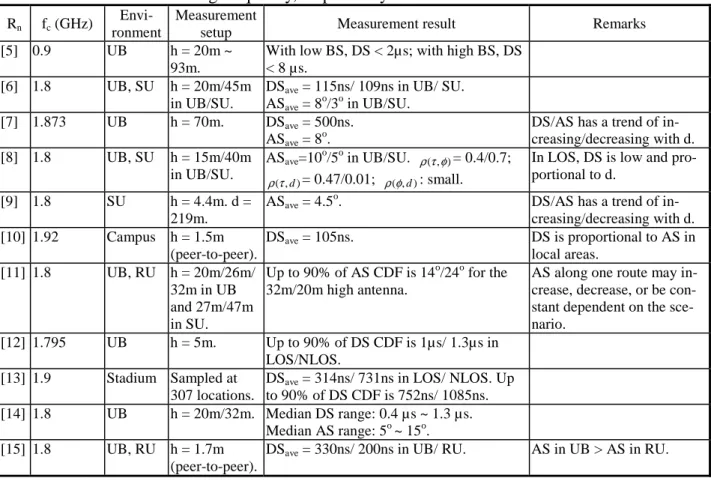
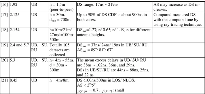
These channel characteristics can be explored by using measurement methods or by using spatio-temporal channel models. Channel sounding is a direct and effective way to measure detail spatio-temporal channel characteristics, which is useful not only for design and evalua-tion of future wideband systems but also for development and validaevalua-tion of spatio-temporal channel models. Many spatio-temporal channel measurement campaigns have been carried out in urban and suburban areas [5-21]. Measured frequencies included 0.9 GHz, 1.8~2.4 GHz, 5.3~5.7 GHz, and 8.45 GHz. Most works focused on the analyses of path loss, DS (r.m.s. delay spread), and AS (r.m.s. azimuthal or angle spread). Based on these studies, DS and AS
in urban area are found to be larger than that in suburban area. In the both areas, these two parameters are increased as the BS antenna height is reduced. In the same area these parame-ters in NLOS (Non Line-of-Sight) situation are larger than those of LOS situation. It was also found that DS increases with d, where d represents the distance between the base station (BS) and the mobile station (MS). However, AS may not have similar trend. According to our study, AS is dependent on many factors such as the propagation distance, street orientations, distri-bution of surrounding-building height, and locations of distant high-rise buildings. The distant high-rise buildings act as dominant reflectors/scatterers and may induce specific arrival paths with large azimuthal angles and long delays.
In these part, auto-correlation of DS/AS is found to be decreased as the distance between the two sample points is increased [9], which is a straight-forward result. In references [8,21-22], it is found that there is slightly correlation between DS/AS and d but positive cross correlation between DS and AS. However, based on our measurement results, it seems that DS/AS and d is correlated, which may be affected by street orientation and mainbeam direction of the an-tenna array. Table 1 summarizes detail DS and AS measurement results found in the above-mentioned references. Based on these studies, it seems that DS and AS and their corre-lation need to be further studied since they depend on some spatial factors such as building distribution and street orientation. In addition to that, despite many measurement campaigns of TOA and AOA for macrocellular radio channels have been reported in these literatures, studies of their joint statistical property are few. Only one related work is found, which inves-tigates the space-time joint property of indoor environments [23].
Table 1-1 Summary of some representative measurement results of DS and AS. UB, SU, and RU represent mesurement sites of urban, suburban, and rural areas, respectively. h and d represent the BS antenna height and BS-MS distance, respectively. Subscripts “ave” and “min” represent the words of average and minimum, respectively. The definition of ρ(α,β) is given in Equation (6). Rn and fc represent reference
num-ber and transmitting frequency, respectively.
Rn fc (GHz)
Envi-ronment
Measurement
setup Measurement result Remarks [5] 0.9 UB h = 20m ~
93m.
With low BS, DS < 2µs; with high BS, DS < 8 µs.
[6] 1.8 UB, SU h = 20m/45m in UB/SU.
DSave = 115ns/ 109ns in UB/ SU.
ASave = 8 o
/3o in UB/SU. [7] 1.873 UB h = 70m. DSave = 500ns.
ASave = 8o.
DS/AS has a trend of in-creasing/decreasing with d. [8] 1.8 UB, SU h = 15m/40m in UB/SU. ASave=10o/5o in UB/SU. ρ(τ,φ)= 0.4/0.7; ) , (τ d ρ = 0.47/0.01; ρ(φ,d): small.
In LOS, DS is low and pro-portional to d.
[9] 1.8 SU h = 4.4m. d = 219m.
ASave = 4.5 o
. DS/AS has a trend of in-creasing/decreasing with d. [10] 1.92 Campus h = 1.5m (peer-to-peer). DSave = 105ns. DS is proportional to AS in local areas. [11] 1.8 UB, RU h = 20m/26m/ 32m in UB and 27m/47m in SU. Up to 90% of AS CDF is 14o/24o for the 32m/20m high antenna.
AS along one route may in-crease, dein-crease, or be con-stant dependent on the sce-nario.
[12] 1.795 UB h = 5m. Up to 90% of DS CDF is 1µs/ 1.3µs in LOS/NLOS.
[13] 1.9 Stadium Sampled at 307 locations.
DSave = 314ns/ 731ns in LOS/ NLOS. Up
to 90% of DS CDF is 752ns/ 1085ns. [14] 1.8 UB h = 20m/32m. Median DS range: 0.4 µs ~ 1.3 µs.
Median AS range: 5o ~ 15o.
[16] 1.92 UB h = 1.5m (peer-to-peer).
DS range: 17ns ~ 219ns AS may increase as DS in-creases. [17] 2.125 UB h = 30m. dmin = 700m. Up to 90% of DS CDF is about 900ns in both cases. Compared measured DS with the computed one by using ray-tracing technique. [18] 2.154 UB h=10m/21m/
27m;d=100m~ 500m.
DSave=1.27µs/ 0.65µs/ 1.19µs for different
antenna heights. [19] 2.4 and 5.7 UB, SU,
RU
Totally 105 datasets are collected.
DSave = 37ns/ 24ns/ 19ns in UB/ SU/ RU.
ASave = 89o/ 81o/ 67o. [20] 5.3 UB, SU, RU h= 4m ~ 55m. d = 30m ~ 300m.
The mean excess delays in UB/ SU/ RU are 38ns ~ 102ns, 36ns, and 29ns. DSs in UB/SU/RU are 44ns ~ 88ns, 25ns, and 22 ns. [21] 8.45 UB h = 4m/8m. DS<100ns/500ns in LOS/ NLOS. AS < 2o/5o. ) , (τφ ρ = 0.7; ρ( dτ, ): small
Here, extended measurement of TOA and AOA was performed in macrocellular urban and suburban environments for up-link communication. The wideband measurement was per-formed at 1.95 GHz of bandwidth 50 MHz by using a wideband vector channel sounder, which is a single-input-multiple-output (SIMO) system. From the measurement data, spa-tio-temporal channel characteristics such as the statistical distributions of TOA, AOA, DS, and AS, and their joint statistical properties are evaluated and discussed.
2. Measurement Setup and Sites
2.1 Measurement system
The RUSK wideband vector channel sounder [24] is employed here to measure directional mobile radio channels. The system diagram of the sounder is illustrated in Figure 1. It consists of a mobile transmitter (Tx) with an omni-directional antenna, and a fixed receiver (Rx) with an 8-element ULA (Uniform Linear Array), where each element is a 0.5 wavelength dipole antenna and the spacing between neighboring elements is 0.4 wavelengths. The effective azi-muth range of the ULA is 120o. The mainbeam of the ULA points a fixed direction during the measurement. Periodic multi-frequency excitation of 50 MHz bandwidth is used, i.e., the time resolution of the system is 20ns. Calibration process of the rubidium reference removes the tracking error of the measurement system and provides a reference plane to ensure the accu-racy of the absolute delay time.
Fig. 1-1 System diagram of the wideband vector channel sounder.
rapid succession. After receiving by the Rx, signals are gathered at the digital receiving unit and sent to a personal computer (PC) to analyze the power, TOA, and AOA of the received impulse response. The AOA is estimated by using Unitary ESPRIT with the sub-array smoothing technology [25]. Then DS and AS represented by notations στ and σφ,
respec-tively, are given by [26]
2 2 τ τ στ = − (1) and 2 2 φ φ σφ= − (2) with 2 2 ( ) ( ) i i i i i P P τ τ τ τ =
∑
∑
and∑
∑
= i i i i i P P ) ( ) ( τ τ τ τ (3) 2 2 ( ) ( ) i i i i i P P φ φ φ φ = ∑ ∑ and ( ) ( ) i i i i i P P φ φ φ φ = ∑ ∑ (4)where P(τi) and P(φi) are the powers of the i-th MPC arriving at the BS with delay τi and
AOA φi, respectively.
2.2 Measurement sites and setup
Extended spatio-temporal channel impulse response measurements were conducted in differ-ent macrocellular environmdiffer-ents, including urban and suburban areas. A summary of meas-urement sites is given in Table 1-2. At each site, the Rx and its antenna were mounted on a rooftop; the Tx and its antenna were carried in a trolley with antenna height of 1.8 meter above the ground. The transmission power is equal to 1W at frequency 1.95 GHz.
Table 1-2 Measurement setup and environments Class h
(m) Numbers of sampled routes and points d (m) Measurement Environment Large City
(Taipei city)
48 Total number of the sampled routes is 9 and each has 500 meters long ap-proximately. Total sampled points are about 1800. Most of them are in NLOS situation.
50~510 Heavily built up area with an average building height of 10 stories. The maximum one is 26 stories. Each story has a height of about 3.5 meter. Small/Med
ium City (Chungli
city)
40 Total number of the sampled routes is 4 and each has 250 meters long ap-proximately. Total sampled points are about 400. Most of them are in NLOS situation.
50~320 Typical urban area with an av-erage building height of 6 sto-ries. The maximum one is 16 stories.
Suburban 27 Total number of the sampled routes is 5 and each has 150 meters long ap-proximately. Total sampled points are about 300. Most of them are in LOS or NLOS situations.
70~360 Small village with buildings of 3~6 stories and gardens with trees and pools.
Fig. 1-2 Layout of six measured routes in Taipei city. The arrow direction of Rx shows the mainbeam direction of the ULA. Paths 1 to 6 are the six measured routes.
Measurement was done along selected routes with a speed of 10 kilometers per hour. Numer-ous parked vehicles and trees were lined along the roads in which many types of buildings were involved such as office buildings, schoolhouses, apartments, stores, etc. These buildings have framed windows and flat roofs of 1 to 26 stories with story height about 3.5 meters. Walls of these buildings are made with bricks, reinforced concrete, and/or glass. The layout of six measured routes in Taipei city is illustrated in Figure 1-2.
3. Measurement Analysis
3.1 TOA and AOA Statistics
3.1.1 Probability density distribution
Well-known statistical models are applied here to study measured TOA and AOA distributions of up-link macrocellular radio channels. An one-sided exponential decaying function and a truncated Laplacian function are adopted to describe TOA’s and AOA’s probability density distributions, respectively [14,27]. The former and latter functions can be written as
) / exp( / 1 ) (τ = στ⋅ −τ στ TOA and ) / | | 2 exp( ) / 2 ( ) (φ = σφ ⋅ − θ σφ AOA , (5)
respectively. In processing the measured data, each MPC in the power delay-azimuth spec-trum is considered if its peak power is greater than –87 dBm and is within 30 dB difference compared with the strongest component of the spectrum due to the dynamic range and sensi-tivity of the sounding system. Note that each local power delay-azimuth spectrum is derived by averaging over the samples measured within a few tens of wavelength.
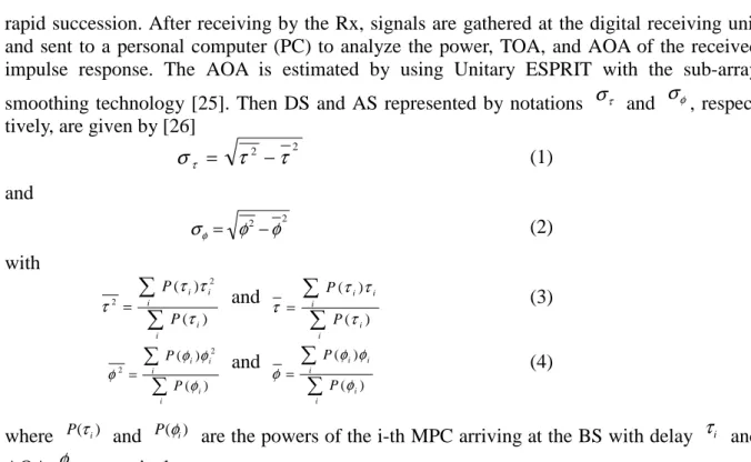
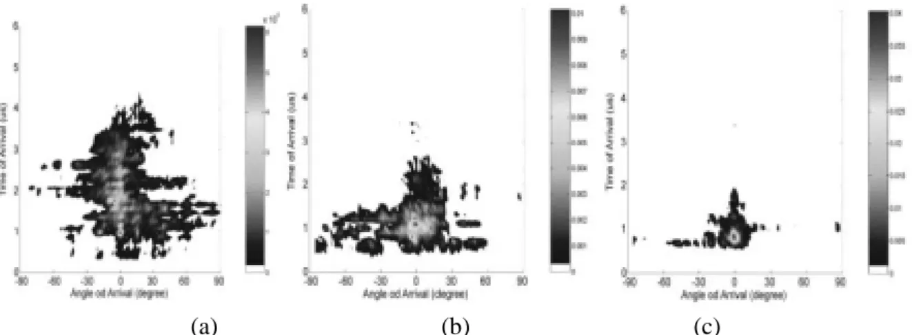
Measured and computed AOA probability density distributions (pdds) in Taipei (a large city), Chungli (a small/medium city about 50 Km away from Taipei), and the suburban area are shown in Figures 1-3(a), 1-3(b) and 1-3(c), respectively. Angle spread measured in Taipei city is the largest among all areas. It is found that the proposed function cannot well match the measured AOA distribution in the urban areas especially in the tail region, which is shown in Figures 1-3(a) and 1-3(b).
(a) (b) (c)
Fig. 1-3 Measured and computed probability density distributions of AOA for (a) Taipei; (b) Chungli; and (c) the suburban area, where dots and solid line represent the measured and computed results, respectively.
To analyze further, AOA distributions with the samples chosen from different excess delay ranges including 601~1200ns and 1801~2400ns, are plotted in Figures 1-4(a) and 1-4(b), re-spectively. It is found that the deviation is increased, especially in the tail region, as the excess delay increases. One of the reasons is that the high-rise buildings, which are localized only in some small areas, act as distant major scatterers and induce significant clustered paths at a specific direction. This phenomenon may be more evident in the case of large propagation range, i.e., with large excess delay, since the effective scattering zone becomes large enough to include more site-dependent high-rise buildings.
(a) (b)
Fig. 1-4 Dashed line represents the histograms of AOA in Taipei city for excess delay ranges at (a) 601~1200ns and (b) 1801~2400ns. The solid line represents the computed probability density distribution of AOA. Long excess delay leads to large deviation. Figures 1-5(a), 1-5(b), and 1-5(c) show the measured and computed TOA probability density distributions in Taipei, Chungli, and the suburban area, respectively. It is observed that the proposed function can fit the measured results well. The measured result shows that multipath propagation in the metropolitan area and the suburban leads the largest and the smallest, mean excess delay and delay spread, respectively. It is consistent with others’ research results [19-20]. It is noted that up to 90% of TOA in Taipei, Chungli, and the suburban area are ap-proximately equal to 2400ns, 1500ns, and 1000ns, respectively. This trend that large cities have larger TOA is similar to that reported in [20]. From these figures, it is observed that the TOA spread in the urban area is much larger than that in the suburban area.
3.1.2 Joint probability density distribution
Figures 1-6(a), 1-6(b), and 1-6(c) show the joint TOA and AOA probability density distribu-tions in Taipei, Chungli, and the suburban area, respectively.
(a) (b) (c)
Fig. 1-5 Measured and computed probability density distributions of excess delay are repre-sented by dots and solid line, respectively, for (a) Taipei City; (b) Chungli; and (c) the suburban area. Mean excess delays in these three areas are 1708ns, 906ns, and 717ns, respectively.
Figure 6 shows a trend that the AOA spreading width is decreased as the TOA is increased. It is because that the number of the effective paths that have large TOA, i.e., with long propaga-tion range, arriving at the Rx through multiple-reflecpropaga-tion-diffracpropaga-tion modes (in transversal plane) is decreased in NLOS situation due to the increase of the number of building blocks (obstacles) between Tx and Rx. Therefore, the path along Tx-Rx direction (in vertical plane) will be dominant as the propagation distance increases since both the number and magnitude of the MPCs propagating through the transversal planes become small, which decreases the azimuthal spreading.
(a) (b) (c)
Fig. 1-6 Probability density distribution of joint TOA and AOA in (a) Taipei City; (b) Chungli; and (c) the suburban area.
To further investigate the joint space and time property, the correlation coefficient between two channel parameters is introduced and given by [9]
(
)(
)
(
) (
)
∑ ∑ ∑ = = = − − − − = N n N n N n n n n n 1 1 2 2 1 ) ( ) ( ) ( ) ( ) , ( β β α α β β α α β α ρ (6)where (n) and (n) are the spatio-temporal channel parameters of the n-th received MPC including TOA, AOA, DS, and AS. α and β are the mean value of (n) and (n), re-spectively. With this equation, the cross-correlation coefficients between TOA and AOA in Taipei, Chungli, and the suburban area are evaluated from the measurement data and are equal to 0.13, 0.15, and 0.11, respectively, which shows that TOA and AOA are slightly correlated.
3.2 r.m.s. Delay Spread (DS) and r.m.s. Azimuth Spread (AS) 3.2.1 Cumulative distribution function
The parameters, DS and AS, measure delay and azimuthal dispersions of radio channel due to multipath propagation. From Figure 1-7(a), which shows the cumulative distribution function (CDF) of the DS, up to 90% of DS are approximately equal to 420ns, 310ns and 150ns, for Taipei, Chungli, and the suburban area, respectively. This trend is consistent with other pre-vious results [19-20]. Notice that the last 10% of DS in the suburban area covers a wide dis-persion range from 150ns to 450ns, which is larger than that of other environments. It reveals the fact that the number of high-rise buildings in the suburban area, which act as the dominant scatterers and may induce those large delay spreads, is smaller than other environments. Therefore, only small chance of large delay spread occurs in the suburban area.
(a) (b)
Fig. 1-7 Measured CDF of (a) DS; and (b) AS in Taipei, Chungli, and the suburban area. Mean DSs in three areas are 278ns, 185ns, and 97ns, respectively; mean ASs in three areas are 18.2o, 16.6o, and 13o, respectively.
The AS in the urban environment is usually larger than that in the suburban environment, which is shown in Figure 1-7(b). Here, up to 90% of AS are approximately equal to 30o, 30o and 24o in Taipei, Chungli, and the suburban area, respectively. It seems that DS is more area-dependent than AS according to the evidence that the relative difference of the three curves in Figure 1-7(a) is much larger than that in Figure 1-7(b).
3.2.2 Joint statistic property
The cross-correlation coefficient between DS/AS and d for the three areas are summarized in Table 1-3. It is observed that there is no strong correlation between DS and d in all areas, which is similar as the results reported in [8] and [21]. However, the correlation between AS and d is higher than DS in three areas. It is also noticed that the correlation between DS/AS and d in the urban area is higher than that in the suburban area.
Table 1-3 Cross-correlation coefficient between DS/AS and d.
Environment α β ρ(α,β)
Large city (Taipei) DS d 0.3833
Small/medium city (Chungli) DS d 0.2993
Suburban DS d 0.0854
Large city (Taipei) AS d 0.4656
Small/medium city (Chungli) AS d 0.4567
Suburban AS d 0.3323
Table 1-4 Cross-correlation coefficient between DS/AS and d versus included angle between the ULA mainbeam direction and that of the sampled route.
Environment Included angle α β ρ(α,β) Large city o 90 = θ AS d 0.6147 Large city o 0 = θ AS d 0.3469 Small/medium city o 90 = θ AS d 0.6195 Small/medium city o 0 = θ AS d 0.2411 Suburban o 90 = θ AS d 0.6341 Suburban o 0 = θ AS d 0.2335 Large city o 90 = θ DS d 0.6333 Large city o 0 = θ DS d 0.4345 Small/medium city o 90 = θ DS d 0.2176 Small/medium city o 0 = θ DS d 0.6712 Suburban o 90 = θ DS d 0.0039 Suburban o 0 = θ DS d 0.1591
It is also found that the cross-correlation between DS/AS and d will be affected by the in-cluded-angle between the ULA mainbeam direction and the direction along the sampled route. In Table 1-4, it is observed that, while the both directions are perpendicular to each other, the correlation between AS and d in both the urban and suburban areas is larger than the case while the both directions are in parallel. It is easy to understand that the AS is decreased with distance in the parallel case since the main propagation paths are confined in the measured street. In the Table, it is also observed that the correlation between DS and d is low in the suburban area and may be high in the urban area dependent on the street orientation.
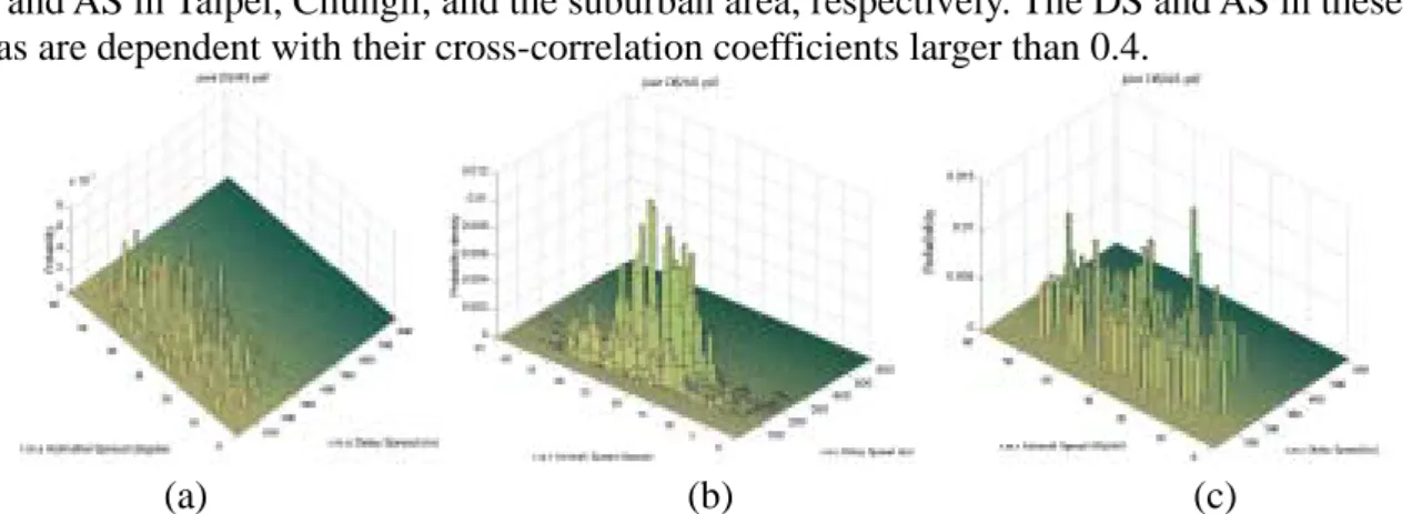
Figures 1-8(a), 1-8(b), and 1-8(c) show the measured joint probability density distributions of DS and AS in Taipei, Chungli, and the suburban area, respectively. The DS and AS in these areas are dependent with their cross-correlation coefficients larger than 0.4.
(a) (b) (c)
Fig. 1-8 Joint probability density distribution of DS and AS for (a) Taipei; (b) Chungli; and (c) the suburban area. The cross-correlation coefficients between DS and AS in these areas are 0.53, 0.44, and 0.41, respectively.
This phenomenon is more evident when the sampled area is narrow down to a route. Figures 1-9(a) and 1-9(b) show the measured DS and AS along Shinyi Road in Taipei, respectively. It is found that along the same route the AS and DS are dependent with their cross-correlation coefficient equal to 0.67. The both figures reveal that DS and AS are correlated with d when d is larger than 100 meters. Figures 1-10(a) and 1-10(b) illustrate the measured DS and AS along Dunhua South Road in Taipei, respectively. In this case, the cross-correlation coeffi-cient between DS and AS is equal to 0.61 and it follows a similar trend (versus d) as that in Figure 1-9.
(a) (b) Fig. 1-9 Measured (a) DS; and (b) AS along Shinyi Road in Taipei city.
(a) (b) Fig. 1-10 Measured (a) DS; and (b) AS along Dunhua South Road in Taipei city.
4. Conclusion
In this chapter, quantitative analysis of spatio-temporal radio channel characteristics has been performed using the extended AOA and TOA measurement data in macrocellular urban and suburban environments. The measurement was carried out by using a wideband vector chan-nel sounder at 1.95 GHz of 50 MHz bandwidth. It is verified that a probability density distri-bution of TOA for urban and suburban environments can be described by using a one-side exponential decaying function. It is also found that a truncated Laplacian function may not well describe the probability density distribution of AOA, especially in the tail region.
Joint statistical property between different channel parameters is studied also. It is found that the AOA spreading width is decreased as the TOA is increased. The cross-correlation between TOA and AOA is low. The DS and AS in urban area are larger than that in the suburban area. These two parameters will be affected by the included angle between the mainbeam direction of the ULA and that of the sampled route. Cross-correlation of DS/AS under different condi-tions is analyzed. Generally, cross-correlation coefficient in the urban area is larger than that in the suburban area. In the same area, the correlation coefficient between AS and d will be higher as the direction of the measured route is perpendicular to that of the ULA mainbeam than the parallel case. However, the correlation between DS and d is not so strong as the for-mer. In the urban area, cross-correlation between DS and AS is high, which is not necessary to be affected by d.
5. References
1. A. M. Vernon, M. A. Beach, and J. P. McGeehan, “Planning and optimization of smart antenna base stations in 3G networks,” IEE Colloquium on Capacity and Range En-hancement Techniques for the Third Generation Mobile Communications and Beyond, pp.1/1-1/7, 2000.
2. L. C. Godara, “Applications of antenna arrays to mobile communications, part I: per-formance improvement, feasibility, and system considerations,” IEEE Proceedings, Vol. 85, No. 7, pp.1031-1060, July 1997.
3. J. C. Liberti and T. S. Rappaport, Smart antenna for wireless communications: IS-95 and third generation CDMA applications, Prentice Hall, Inc., 1999.
4. K. H. Li, M. A. Ingram, and A. V. Nguyen, “Impact of clustering in statistical indoor propagation models in link capacity,” IEEE Trans. Commun., Vol. 50, pp.521-523, April 2002.
5. S. Y. Seidel, T. S. Rappaport, S. Jain, M. L. Lord, and R. Singh, “Path loss, scattering, and multipath delay statistics in four European cities for digital cellular and microcellular ra-diotelephone,” IEEE Trans. Veh. Technol., Vol. 40, No. 4, pp.721-730, November 1991. 6. U. Martin, “Spatio-temporal radio channel characteristics in urban macrocells”, IEE Proc.
Radar, Sonar Navig., Vol. 145, No. 1, p.42-49, Feb 1998.
7. M. Larsson, “Spatio-temporal channel measurements at 1800 MHz for adaptive anten-nas,” IEEE VTC, Vol. 1, p.376-380, July 1999.
8. M. Nilsson, B. Lindmark, M. Ahlberg, M. Larsson, and C. Becjman, “Measurements of the spatio-temporal polarization characteristics of a Radio channel at 1800 MHz,” IEEE VTC, Vol. 1, p.386-391, July 1999.
9. J. Takada, J. Fu, H. Zhu, and T. Kobayashi, “Spatio-temporal channel characterization in a suburban non line-of-sight micocellular environment,” IEEE J. Select. Areas Commun., Vol. 20, No. 3, pp.532-538, April 2002.
10. G. D. Durgin, V. Kukshya, and T. S. Rappaport, “Joint angle and delay spread statistics for 1920 MHz peer-to-peer wireless channels,” IEEE International Sym. Antennas Propa-gat., Vol. 2, pp.182-185, 2001.
11. K. I. Pedersen, P. E. Mogensen, and B. H. Fleury, “Spatial channel characteristics in out-door environments and their impact on BS antenna system performance,” IEEE VTC, Vol. 2, pp.719-723, May, 1998.
12. G. V. Tsoulos and G. E. Athanasiadou, “On the application of adaptive antennas to mi-crocellular environments: radio channel characteristics and system, performance,” IEEE Trans. Veh. Technol., Vol. 51, No. 1, pp.1-16, January 2002.
13. N. Moraitis, A. Kanatas, G. Pantos, and P. Constantinou, “Delay spread measurement and characterization in a special propagation environment for PCS microcells,” IEEE The 13th International Sym. Personal, Indoor and Mobile Radio Commun., Vol. 3 pp.1190-1194, 2002.
14. K .I. Pedersen, P. E. Mogensen, and B. H. Fleury, “A stochastic model of the temporal and aziumthal dispersion seen at the base station in outdoor propagation environments,” IEEE Trans. Veh. Technol., Vol. 49, No.2, pp.437-447, March 2000.
15. N. Patwari, G. D. Durgin, T. S. Rappaport, and R. J. Boyle, “Peer-to-peer low antenna outdoor radio wave propagation at 1.8 GHz,” IEEE The 49th VTC, Vol. 1, pp.371-375, May 1999.
16. G. D. Durgin, Ph.D. Thesis: Theory of Stochastic local area channel modeling for Wire-less Communications, Virginia Polytechnic Institute and State University, 2000.
17. T. Rautiainen, G. Wolfle, and R. Hoppe, “Verifying path loss and delay spread predictions of a 3D ray tracing propagation model in urban environments,” IEEE VTC, Vol. 4, pp.2470-2474, 2002.
18. J. Laurila, K. Kalliola, M. Toeltsch, K. Hugl, P. Vainikainen, and E. Bonek, “Wide-Band 3-D characterization of mobile radio channels in urban environment,” IEEE Trans. An-tennas and Propagat., Vol. 50, No. 2, p.233-243, Feb 2002.
19. G. Woodward, I. Oppermann, and J. Talvitie, “Outdoor-indoor temporal & spatial wide-band channel model for ISM wide-bands,” IEEE VTC, pp.136-140, May 1999.
20. X. Zhao, J. Kivinen, P. Vainikainen, and K. Skog, “Propagation characteristics for wide-band outdoor mobile communications at 5.3 GHz,” IEEE J. Select. Areas Commun., Vol. 20, No. 3, p.507-514, April 2002.
21. H. Masui, M. Ishii, K. Sakawa, H. Shimizu, T. Kobayashi, and M. Akaike, “Spa-tio-temporal channel characteristics at base station in microwave urban propagation,” URSI The 18th National Radio Science Conference, pp.F2/1-F2/7, March 2001.
22. A. Algans, K. I. Pedersen, and P. E. Mogensen, “Experimental analysis of the joint statis-tical properties of azimuth spread, delay spread, and shadow fading,” IEEE J. Select. Ar-eas Commun., Vol. 20, No. 3, pp.523-531, April 2002.
23. C. C. Chong, C. M. Tan, D. I. Laurenson, S. McLaughlin, M. A. Beach, and A. R. Nix, “A new statistical wideband spatio-temporal channel model for 5-GHz band WLAN sys-tems,” IEEE J. Select. Areas Commun., Vol. 21, No. 2, pp.139-150, February 2003. 24. R. S. Thoma, D. Hampicke, A. Richter, G. Sommerkorn, A. Schneider, U. Trautwein, and
W. Wirnitzer, “Identification of time-variant directional mobile radio channels,” IEEE Trans. Instrum. Meas. Technol., Vol. 49, No. 2, pp.357-364, April 2000.
25. H. Krim and M. Viberg, “Two decades of array signal processing research,” IEEE Signal Processing Mag., Special Issue on Array Processing, Vol. 13, July 1996.
26. T. S. Rappaport, Wireless Communications: Principles and Practice, Prentice-Hall, Inc., New Jersey, 1996.
27. J. B. Andersen and K. I. Pedersen, “Angle-of-arrival statistics for low resolution anten-nas,” IEEE Trans. Antennas Propagat., Vol. 50, No. 3, pp.391-395, March 2002.
PART II A Physical and a Physical-Statistical
Spa-tio-Temporal Radio Channel Model for
Macro-cellular Environments
Abstract
This part presents a new hybrid spatio-temporal channel model for macrocellular radio chan-nels in urban environments, which combines a 3-D (Three-dimensional) site-specific model with a statistical model. The former model employs a deterministic approach with the ray-tracing method to describe the direct wave, specular reflection waves, and single and mul-tiple-over-rooftop diffracted waves. The latter model applies a statistical approach to describe scattered fields due to local scatterers around mobile stations and effective scatterers on the illuminated walls of dominant buildings. It is proposed that the effective scatterers are uni-formly distributed on the walls with a given effective scatterer number density, which is de-termined by a measurement-based method. By comparing the computed TOA (Time-of-Arrival), AOA (Angle-of-Arrival), r.m.s. angle spread and r.m.s. delay spread of multipath propagation in urban environment with the measured ones, the hybrid spa-tio-temporal radio channel model has been proved to be effective and accurate.
1. Introduction
To add the capacity of third-generation-and-beyond communication systems, smart antennas have utilized the SDMA (Space Division Multiple Access) technique [1]. The technique adap-tively processes the transmitting array signal at base stations (BS) to increase the signal gain of a mobile receiver by pointing its main beam toward that receiver and to reduce the overall interference by pointing its nulls to other mobile receivers [2]. For the radio communication systems with SDMA, the spatial distribution of the multipath components is important to de-termine the performance of the radio link [3]. Therefore, to apply this technique, spatial and temporal dispersions of radio channels are required, which can be provided by spa-tio-temporal radio propagation models.
Many spatio-temporal models have been developed based on either simple geometric or measurement models and most of them are statistical models. Overview of these models is given in [4]. In Lee’s model [5], effective scatterers distribute uniformly in a circle ring whose center is the mobile station and radius is 100~200 wavelength. The effective scatterer repre-sents the effect of many scatterers within a region. The Geometrically Based Circular Model (GBCM) for macro-cellular environment assumes that scatterers distribute within a circle whose center is the mobile station (MS) with a chosen radius [6-7]. In Gaussian Wide Sense Stationary Uncorrelated Scattering (GWSSUS) model, scatterers are grouped into many clus-ters [8-11]. However, GWSSUS model does not indicate how to decide the number and the location of clusters. Raleigh’s model [12-13] that is called time-varying vector channel model provides small scale Rayleigh fading and theoretical spatial correlation properties. The propagation environment considered in Raleigh’s model is densely populated with large dominant reflectors. The above models employ a statistical approach and cannot describe the channel characteristics for specific sites. The site-specific model [14-17] applying the ray-tracing method, a deterministic approach, can overcome this deficiency. However, the site-specific model fails to properly describe the effects of randomly positioned scatterers and diffuse scattering phenomena, which may have a significant impact on the random nature of received fields.
pre-sented by combining a 3-D site-specific deterministic model with a geometrically based sta-tistical model. The former model describes the direct wave, specular reflection waves, and single and multiple-over-rooftop diffracted waves due to ground, building walls and edges with a deterministic approach. However, it neglects the scattered fields due to randomly posi-tioned local scatterers around the mobile station (MS), and due to scattered objects being parts of the buildings such as windows, decorative masonry, electric cables, heating pipes, etc. The latter scattered fields may be dominant in the received signal especially in the NLOS (Non Line-of-Sight) propagation situation. Measurement results also show that the multipath com-ponents due to these scatterers arrive in groups. In each group, the paths are clustered in space-time domain [18]. Therefore, the latter model applies a statistical approach to describe scattered fields due to local scatterers around mobile stations and effective scatterers on the illuminated walls of dominant buildings. It is proposed that the effective scatterers are uni-formly distributed on the walls with a given effective scatterer number density, which is de-termined by a measurement-based method.
With employing a physical and statistical approach, the hybrid model can effectively predict the field point-by-point by using the site-specific model and can describe the random effect due to the environment by using the statistical model. Hence the model may be linked to spe-cific locations because of its deterministic nature or may be applied to a general situation be-cause of its statistical nature.
2. Measurement Setup, Sites and Data Analysis
A. Measurement Setup
For measurement of time-varying and directional mobile radio channels, a RUSK vector channel sounder is employed [19], whose system diagram is illustrated in the Figure 2-1. The sounding system consists of a mobile transmitter (Tx) with an omni-directional antenna, and a fixed receiver (Rx) with an 8-element ULA (Uniform Linear Array), where each element is a 0.5 wavelength dipole antenna and the spacing between neighboring elements is 0.4 wave-length. Periodic multi-frequency excitation with 120MHz bandwidth is used, i.e., the time resolution is 8.3ns. The Doppler bandwidth of 20kHz allows complete statistical analysis of the time-varying radio channel with respect to different azimuthal directions of the impinging waves. Tx/Rx synchronization is maintained by two rubidium references. Calibration process of the rubidium reference removes the tracking error of the measurement system and provides a reference plane to ensure the accuracy of the absolute delay.
The channel impulse responses of the antenna array are recorded as “vector snapshots” in rapid succession. After receiving by Rx, signals are gathered at the DRU (Digital Receiving Unit) and are sent to a PC (personal computer) to analyze the received power, TOA (Time-of-Arrival), and AOA (Angle-of-Arrival) of the received impulse response. The AOA is estimated by using Unitary ESPRIT with the sub-array smoothing technology. An overview about array signal processing including the estimation of the AOA and a comparison of ES-PRIT with other algorithms can be found in [20].
The receiving array antenna was mounted on a rooftop with the transmission power 1W at frequency 2.44 GHz. The Tx antenna was carried in a trolley at a height of 1.8 meter above the ground. Measurement was done at fixed points and along selected routes with a walking speed. The measurements were carried out between 10:00 A.M.~ 8:00 P.M. with pedestrians around and vehicles passing by.
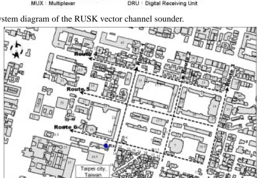
roads in Taipei city and the layout of the measured routes is shown in Figure 2-2. In the figure, the position of ULA, i.e., Rx, is shown, which was located on a roof of 40 meter height above the ground. The main beam of the ULA was set to point a fixed direction during the meas-urement. The propagation condition along each route is listed in Table 1. Numerous parked vehicles and trees were lined along the roads. Many types of buildings were involved such as office buildings, schoolhouses, apartments, stores, etc. These buildings have framed windows and flat roofs of 1 to 17 stories height with 3.5 meters height of each story. Walls of these buildings were made with materials such as brick, concrete, and/or glass.
C. Measurement Analysis
(a) Propagation modes
Figures 2-3(a) and 2-3(b) show time variant AADS (Aperture Averaged Delay Spectrum) and DAAS (Delay Averaged Azimuth Spectrum) measurement results along route 1. The AADS is calculated by averaging the squared magnitude of the impulse response over all the array elements. The impulse response is computed by using the inverse Fourier transformation of the measured complex frequency transfer function [19]. The DAAS is computed by averaging the squared magnitude of delay-azimuth spectrums (DASs) over delay time. Here, a de-lay-azimuth spectrum is determined by processing a set of eight-array element impulse re-sponses with the Unitary ESPRIT algorithm.
It is observed that the direct path has the largest received power, as shown in Figure 2-3(a) and Group A in Figure 2-3(b). The paths with long delay time shown in Figure 2-3(a), corre-sponding to the paths shown in Group B of the Figure 3(b), are due to multiple-reflection of the street walls. Figure 2-4(a) shows the measured DAAS along route 2, which is alone the street with similar building heights of the both sides. Two received path groups (Groups A and B) are observed, which have similar angle dispersions but different AOAs. The ray-tracing method using in the site-specific model can predict their path trajectories as shown in Figure 2-4(b). It is found that Group A is resulted from the rooftop-diffracted waves (path trajectory Tx-D1-Rx, shown in Figure 2-4(b)), and the wave reflected by the walls and then diffracted by the rooftop produces Group B (path trajectory Tx-B-D2-Rx). Group C represented the corner-diffracted waves due to distant high-rise buildings (path Tx-E-Rx). It is noted that the other two propagation paths, Tx-D1-Rx and Tx-C-D1-Rx, have the same azimuthal angle, and may not be distinguishable and are clustering together if their propagation delay difference is small.
From the measurement results, several major propagation mechanisms are observed, which include (1) the direct wave; (2) multiple-reflected waves; (3) waves guided by street canyons; (4) waves diffracted over multiple-rooftop; and (5) waves reflected and scattered by high-rise buildings. The first two modes are important for LOS propagation and the last four modes are critical to NLOS propagation. With these major mechanisms, macrocellular channel models can be simplified, especially for the site-specific model shown in the section 3.B.
(b) DAS cluster phenomenon
To investigate DAS cluster phenomenon, measurement of DAS in a simple propagation envi-ronment was conducted. Geometry of the BS and the MS positions and propagation environ-ment are shown in Figure 2-5(a). With the measured DAS shown in Figure 2-5(b), three ob-vious DAS clusters I, II and III are found. In each cluster, the region with lighter color repre-sent the stronger field strength. To analyze the cause of these clusters, the ray-tracing method is applied to trace the propagation paths and to determine the positions of associated re-flected-points or diffracted-points on the building. The result shows that peak A of cluster I
and peak B of cluster III are due to the direct wave and the specular reflected wave of the building wall, respectively. The geometry of the traced paths is shown in Figure 2-5(a). Therefore, DAS cluster I is interpreted as the summation of the direct wave and its scattered waves by the local scatterers around the MS. DAS cluster II represents the diffused/reflection waves due to ground. The specular reflected wave of the building wall and the scattered waves due to building edges and the objects being part of the building such as windows, bricks, electric cables, etc., yield DAS cluster III.
Notice that, in Figure 2-5(b), the measured maximum time dispersion of the DAS cluster III is equal to 0.096µs, which is also equal to the maximum TOA difference between paths 1 and 2 as shown in Figure 2-5(a), and these two paths have arrived at the BS with the same azimuthal angle. So, their TOA difference depends on the vertical dimension of the reflected wall. Fur-thermore, the angle dispersion of DAS cluster III is approximately 110 degrees, which is de-termined by the horizontal view angle of the reflected wall seen from the BS. Hence, the ver-tical and horizontal dimensions of the reflected wall can determine the time and angle disper-sions of the DAS cluster, respectively.
(c) Spatial channel modeling and validation
According to the above analysis, it is found that most multipath components of DAS cluster III are mainly due to building-wall reflection. The diffraction wave of the building edge, which is not so obvious compared with other scattered waves due to the discontinuities on the wall, may be considered together with the wall reflection and scattering. Therefore, it is pro-posed that the size of effective scattering zone is equal to the wall size of the dominant build-ing. Scattering effect of the zone can be modeled by introducing effective scatterers into it, which forms a scatterer cluster [3]. It is assumed that effective scatterers are uniformly dis-tributed on the whole wall surface. Figures 2-6(a) shows the comparison between measured and computed DASs due to scattering of the dominant wall surface when the MS is located on the extended center axis of the building surface. The shaded area in the figure, i.e., the com-puted DAS, is determined by inserting uniformly distributed scatterers with density of 1 scat-terer per unit meter square. The comparison result illustrates that our spatial channel model can properly predict the received DAS. Similar results are found in Figures 2-6(b) and 6(c), where the MS is moved to the left and right sides of the extended center axis, respectively. The DAS cluster center is moved and its shape is changed as the MS moves.
3. The Hybrid Spatio-Temporal Channel Model
A. Hybrid Model
In the present hybrid model, the received electric field after the antenna is determined by a superposition of deterministic and randomly scattered statistical rays, which is given by
sr dr r
E
E
E
=
+
( 1 ) where∑
⋅ = i di dr E E ρv* v. Edr represents the summation of each deterministic ray field Edi v
, which is computed by the site-specific model. ρv* is the complex conjugation of unit polari-zation vector of the receiving antenna. Esr represents the summation of the scattered fields. The scattered field is due to the local scatterers around the MS and the effective scatterers on the wall surfaces of the dominant buildings. The geometry of deterministic and random rays of the hybrid model is illustrated in Figure 2-7. The effective scatterers are uniformly
distrib-uted on the whole scattering wall surface, the gray area in the figure. Here, single-bounce as-sumption is made [21-22].
B. 3-D site-specific model
The 3-D site-specific model includes multipath propagation in both vertical and transversal planes [14-17]. The vertical plane is defined by the transmitter and the receiver positions and is perpendicular to the earth surface, where propagation paths due to direct wave, ground-reflected wave, and multiple rooftop-diffracted waves are considered. The transversal plane is perpendicular to the vertical plane, where propagation paths due to wall-reflected waves and corner-diffracted waves are considered. The complex received field of i-th ray propagating on the vertical plane or transversal plane is given by
∏
⋅ ⋅ ⋅ ⋅ ⋅ = j ij d i ri ti di E G G L d f D E 0 ( ) ( 2 ) or∏
Γ ⋅ ⋅ ⋅ ⋅ ⋅ ⋅ = j ij r i D i ri ti di E G G L d L f E 0 ( ) (φ ) ( 3 ) respectively. E0 is the electric field one meter away from the transmitting antenna, Gti andri
G
are the field-amplitude radiation patterns of the transmitting and the receiving antennas, respectively. Li(d) and LD(φi) are the path loss with a unfold length d and the corner dif-fraction loss with a difdif-fraction angle φi[23], respectively.
∏
jij
D
is used to compute the mul-tiple diffraction over the rooftops and the method of RTM (Ray-Transmission Matrix) is
em-ployed [24].
∏
Γj ij
computes multiple-reflected waves by walls. Since some of the energy is scattered by the effective scatterers, fr and fd are the attenuation factors due to diffused reflec-tion and multi-diffracreflec-tion [25], respectively. These losses can be included in the scattering field. The ray-fixed coordinate systems and the edge-fixed coordinate systems [26-27] are applied in evaluation of reflection and diffraction coefficients, respectively. In the LOS situa-tion, the ground-reflected wave is considered and is given by
g d i ri ti di E G G L d f E = 0⋅ ⋅ ⋅ ( )⋅ ⋅Γ (4) where Γg is the ground-reflection coefficient. Equation (4) can represent the direct wave by setting Γg =1 and fd = 1.
The objects such as buildings in cellular environments are modelled by a number of facets and edges of the order of several hundreds. The ray tracing technique is used to trace the ma-jor propagation paths from the transmitter location to the receiver location and the image method is applied to determine the intersections of rays and the objects of the environment, which will be used repeatedly many times in the computation.
Note that, according to reference [28], the authors found that the effect of double diffraction in the transversal plane is much smaller than that of single diffraction and other double effects such as double reflection, which is verified by comparing the computation and measurement
results. The authors also claimed that it would take much longer computational time if the double diffraction is considered. Hence, based on the measurement result analysis in section II.C and to save the computational time, only the dominant propagation modes, except double diffraction in the transversal plane, are considered in the proposed model.
C. Statistical model sr E is given by local M i i c sr E E E =
∑
+ =1 ( 5 ) where i c Erepresents the scattered field due to the i-th scattering wall surface. M represents the total number of scattering walls, whose positions are determined the ray-tracing method applied in the site-specific model.
i c E is given by
∑
= = Neffi n n i c i c S a E , 1 (6) where di i c E S =is the maximum effective scattered field strength from i-th wall surface. an represents the complex scattering coefficient due to n-th scatterer on the associated wall sur-face. It is assumed to have uniformly distributed amplitude and phase in (0,1) and (0,2 ), re-π spectively. Neff represents the total number of effective scatterers on the associated wall surface.
local
E
is the scattered field due to the local scatterers around the MS such as pedestrians and vehicles. The local scatterers are assumed to distribute uniformly in a sphere centered at the MS [6-7,21-22]. Here, its diameter is assumed to be equal to the width of the street where the MS is located. The formulation of Elocal is the same as that of
i c E except that i c S is re-placed by the direct wave for the LOS situation or the multiple rooftop-diffracted wave for the NLOS situation.
From the analysis of the DAS cluster phenomenon, the total number of effective scatterers on each wall surface is given by
scatterer
eff D
N =∆
θ
⋅∆τ
⋅ ( 7 ) where ∆θ and ∆τ =h /c represent the maximum angular and time dispersions dependent on the horizontal and the vertical dimensions of the associated wall, respectively. ∆θ is de-termined by the width of the associated wall, whose height is equal to h. c is the light speed in free space. Dscatterer is the effective scatterer number density (ESND) per unit delay⋅angle. Several investigations [21-22] have suggested values for the size of the scattering zone and the number of effective scatterer. However, it seems that value of these parameters have not been verified with conscientious experiments.D. ESND (Effective Scatterer Number Density)
ESND is determined by a measurement-based method and the procedure to determine one sampled value is given as following:
(1) Recognize DAS clusters from a measured time average delay-azimuth spectrum at a sampled point.
(2) Identify how many peaks in each DAS cluster and its size.
(3) Assume that each identified peak is due to one scatterer, since single bounce as-sumption is made. Hence, the total number of scatterers is equal to the total number of the identified peaks in a cluster.
(4) Calculate sampled ESND with the scatterer number divided by the corresponding DAS cluster size.
It is noted that the total number of the peaks in procedure (2) is varied with the signal band-width. Mean value of Dscatterer versus the signal bandwidth is shown in Figure 2-8, which has been averaged over approximately 2000 samples taken from the measurement data along routes 2~5. It is observed that mean value of Dscatterer is proportional to the signal bandwidth. Notice that the procedure above can also be applied to determine the ESND of the MS local scatterer.
E. Comparison of the computed and measured results
Computed and measured PASs (power azimuth spectrums) at a sampled point of route 2 are shown in Figures 2-9(a) and 2-9(c), respectively. From the comparison, the site-specific model shows a good prediction accuracy since the computed pulse peaks a~f match the meas-ured one well. In the subfigure of Figure 2-9(a) the trajectory of major propagation paths de-termined by the ray-tracing method is shown, which helps in determining the cause of the re-ceived peaks. With the computed and the measured PDSs (power delay spectrums) shown in Figures 2-9(b) and 2-9(d), respectively, the DAS cluster phenomenon was obvious in the ex-perimental result when comparing cluster group b in the both figures. The comparison dem-onstrates that the site-specific model can predict accurately the AOAs and TOAs of the major paths but may not predict the DAS cluster phenomenon. Figures 2-9(e) and 2-9(f) illustartes one sample of PAS and PDS computed by using the statistical sub-model, respectively. Here, both fr and fd are equal to 0.67, which is determined from our measurement result and its magnitude is similar as that in [25].
F. Validation of Hybrid Model
The hybrid model is validated by comparing computed r.m.s. AS (root mean square of angle spread) and r.m.s. DS (root mean square of delay spread) with the measured ones. Definitions of r.m.s. DS (στ) and r.m.s. AS (σθ ) can be found in [26]. Since the four measured routes (routes 2~5) have been selected to analyze the DAS cluster phenomenon and to determine the mean value of Dscatterer as shown in Figure 2-8, the left measurement data (routes 1 and 6) is used to validate the hybrid model (the blind test approach is adopted).
Computed and measured r.m.s. AS and r.m.s. DS along route 1 are shown in Figures 2-10(a) and 2-10(b) as a function of the measured distance D, respectively. In Figure 2-10(a), r.m.s. AS computed by the site-specific model has the similar trend as the measured one but the model underestimates the result since no scattering effect is considered. It is observed that the
result computed by the hybrid model matches measured result well because that the scattering effect due to the scatterer cluster is included. Note that, from Figure 2-8, Dscatterer is equal to
) /(
184 µs⋅rad
of 120 MHz signal bandwidth. Since most sampled points along this route are in LOS situation, the direct wave is dominant in the received field and the scattering and dif-fused-reflection effects have been suppressed. Therefore, r.m.s. AS and r.m.s. DS computed by the both models are close to the measured result.
Computed and measured r.m.s. AS and r.m.s. DS along route 6 (NLOS propagation) are shown in Figures 2-11(a) and 2-11(b), respectively, as a function of the measured distance. The figure reveals obviously that the hybrid model has a better prediction accuracy than the site-specific model.
Based on the above comparisons, although the improvement of the hybrid model is not much, it is believed that the hybrid approach will not only make channels close to reality but also will add a dimension in exploring the random nature of radio channels. It will be helpful to enable some advanced technologies such as smart antennas and MIMO (Multi-ple-Input-Multiple-Output), which need spatial and spatial-temporal characterization and their joint behavior of the signal propagating through random channels.
4. Conclusion
This part presents a new hybrid (physical and statistical) spatio-temporal radio channel model for the macrocellular environment in urban areas. The model not only accurately estimates the channel parameters such as TOA, AOA, r.m.s. DS, and r.m.s. AS but also adds a dimension in exploring the random nature of radio channels. It combines a 3-D site-specific model with a statistical model. The former model using the ray-tracing method can accurately predict TOAs and AOAs of dominant multipaths such as direct, reflected, and diffracted waves. The latter model applies a statistical approach to describe scattered fields due to local scatterers around mobile stations and effective scatterers uniformly distributed on the scattering walls of domi-nant buildings. These fields are observed as the DAS cluster phenomenon in spatial and tem-poral domains through measurement. In our model, the effective scatterer number of the asso-ciated scattering walls varies when the MS moves, which is different from the previous pro-posed papers [21-22] and could be applied for different macrocellular environments. By comparing the computed spatio-temporal channel characteristics such as TOA, AOA, r.m.s. DS, and r.m.s. AS with the measured ones, the hybrid model is proved to be an effective and accurate spatio-temporal radio channel model.
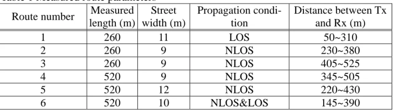
Table 1 Measured route parameters Route number Measured
length (m) Street width (m) Propagation condi-tion Distance between Tx and Rx (m) 1 260 11 LOS 50~310 2 260 9 NLOS 230~380 3 260 9 NLOS 405~525 4 520 9 NLOS 345~505 5 520 12 NLOS 220~430 6 520 10 NLOS&LOS 145~390
Fig. 2-1 System diagram of the RUSK vector channel sounder.
Fig. 2-2 Layout of six measured routes in Taipei city, where the height of each building along the roads is marked (unit: meter). The arrow direction of Rx shows the main beam direction of the ULA.
(a) (b)
Fig. 2-3 (a) Time variant aperture averaged delay spectrum (AADS) along route 1. (b) Time variant delay averaged azimuth spectrum (DAAS) along route 1.
(a) (b)
Fig. 2-4 (a) Time variant DAAS along route 2. (b) Ray trajectory of the propagation paths at the sampled point corresponding to the measured position.
(a)
(b)
Fig. 2-5 (a) Geometry of propagation environment. Several major propagation paths are shown. (b) DAS clusters I, II, and III are shown. Each cluster is resulted from the di-rect/reflected/diffracted/scattered waves having similar spatio-temporal
characteriza-(a)
(b)
(c)
Fig. 2-6 (a) Measured and computed DASs due to scattering of the dominant wall surface when the MS is located on the extended center axis of the building surface. (b) Measured and computed DASs when the MS moved to the left side of the extended center axis. (c) Measured and computed DASs when the MS moved to the right side of the extended center axis. The shape and size of DAS change when the MS is moved.
Fig. 2-7 Effective scatterer density geometry of the hybrid model. The effective scatterers are assumed uniformly distributed in the effective scattering zones (the gray areas). These zones include dominant building walls and local area around the MS.
Fig. 2-8 Mean value of Dscattererversus transmitted signal bandwidth. The dash line is the lin-ear regression fitting line.
(a) (b)
(c) (d)
(e) (f)
Fig. 2-9 Computed and measured results of spatio-temporal channel characteristics at a sam-pled point of route 2. (a) Computed power-azimuth spectrum by the site-specific model; (b) Computed power-delay spectrum by the site-specific model; (c) Measured power-azimuth spectrum; (d) Measured power-delay spectrum; (e) A sample of computed power-azimuth spectrum by the statistical model; (f) A sample of com-puted power-delay spectrum by the statistical model.
0 5 10 15 20 25 0 20 40 60 80 100 120 140 160 180 200 220 240 260 D(m) r. m .s . A n g le S p re ad (d eg re e) Site-specific model Measured Hybrid model (a) 0 20 40 60 80 100 120 140 160 180 0 20 40 60 80 100 120 140 160 180 200 220 240 260 D(m) r. m .s . De la y S pr ea d( ns ) Site-specific model Measured Hybrid model (b)
Fig. 2-10 Computed and measured (a) r.m.s. angle spread and (b) r.m.s. delay spread versus measured distance D along route 1.
0 5 10 15 20 25 30 35 0 20 40 60 80 100 120 140 160 180 200 220 240 260 280 300 320 340 360 380 400 420 440 460 480 500 D(m) r. m .s . A ng le S pr ead (d eg re e) Site-specific model Measured hybrid model (a) 0 20 40 60 80 100 120 0 20 40 60 80 100 120 140 160 180 200 220 240 260 280 300 320 340 360 380 400 420 440 460 480 500 D(m) r. m .s . De la y S pr ea d( ns ) Site-specific model Measured Hybrid model (b)
Fig. 2-11 Computed and measured (a) r.m.s. angle spread and (b) r.m.s. delay spread versus measured distance D along route 6.
5. References
[1] A. M. Vernon, M. A. Beach, and J. P. McGeehan, “Planning and optimisation of smart antenna base stations in 3G networks,” IEE Colloquium on Capacity and Range En-hancement Techniques for the Third Generation Mobile Communications and Beyond, pp.1/1-1/7, 2000.
[2] L. C. Godara, “Applications of antenna arrays to mobile communications, part I: per-formance improvement, feasibility, and system considerations,” IEEE Proceedings, Vol. 85, No. 7, pp.1031-1060, July 1997.
[3] J. C. Liberti and T. S. Rappaport, Smart antenna for wireless communications: IS-95 and third generation CDMA applications, Prentice Hall, Inc., 1999.
[4] R. B. Ertel, P. Cardieri, T. S. Rappaport, and J. H. Reed, “Overview of spatial channel models for antenna array communication systems,” IEEE Personal Communications, pp.10-22, February 1998.
[5] W. C. Y. Lee, Mobile Communications Engineering, McGraw Hill Publications, New York, 1982.
[6] R. B. Ertel, “Statistical analysis of the geometrically based single bounce channel mod-els,” unpublished notes, May 1997.
[7] S. P. Stapleton, X. Carbo, and T. Mckeen, “Spatial channel simulator for phased arrays,” IEEE VTC, Vol. 3, pp.1789-1792, June 1994.
[8] P. Zetterberg and B. Ottersten, “The spectrum efficiency of a basestation antenna array system for spatially selective transmission,” IEEE VTC, Vol. 3, pp.1517-1521, June 1994.
[9] P. Zetterberg and P. L. Espensen, “A downlink beam steering technique for GSM/ DCS1800/PCS1900,” IEEE PIMRC, Taipei, Taiwan, October 1996.
[10] P. Zetterberg, P. L. Espensen, and P. Mogensen, “Propagation, beamsteering and uplink combining algorithms for cellular systems,” ACTS Mobile Commun. Summit, Granada, Spain, November 1996.
[11] U. Martin and M. Grigat, “A statistical simulation model for the directional mobile radio channel and its configuration,” IEEE Proc. 4th International symposium on spread spec-trum techniques and applications, pp.86-90, 1996.
[12] P. Zetterberg, “Mobile communication with base station antenna arrays propagation modeling and system capacity,” Tech. Rep., Royal Inst. Technology, January 1995.
[13] G. G. Raleigh and A. Paulraj, “Time varying vector channel estimation for adaptive spa-tial equalization,” IEEE Proc. Globecom., pp.218-224, 1995.
[14] G. Liang and H. L. Bertoni, “A new approach to 3-D ray tracing for propagation predic-tion in cities,” IEEE Trans. Antennas Propagat., Vol. 46, No. 6, pp.853-863, June 1998. [15] T. Kurner, D. J. Cochom, and W. Wiesbeck, “Concepts and results for 3-D digital
ter-rain-based wave propagation models: an overview,” IEEE J. Select. Areas Commun., Vol. 11, No. 7, pp.1002-1012, September 1993.
[16] E. K. Tameh, A. R. Nix, and M. A. Beach, “A 3-D integrated macro and microcellular propagation model, based on the use of photogrammetric terrain and building data,” IEEE VTC, pp.1957-1961, 1997.
[17] T. S. Rappaport, S. Y. Seidel, and K. R. Schaubach, “Site-specific propagation for PCS system design,” in Wireless Personal Communications, M. J. Feuerstein, T. S. Rappaport, eds., Boston: Kluwer academic publishers, pp.281-315, 1993.
3-D characterization of mobile radio channels in urban environment,” IEEE Trans. An-tennas Propagat., Vol. 50, No. 2, pp.233-243, February 2002.
[19] R. S. Thoma, D. Hampicke, A. Richter, G. Sommerkorn, A. Schneider, U. Trautwein, and W. Wirnitzer, “Identification of time-variant directional mobile radio channels,” IEEE Trans. Instrum. Meas. Technol., Vol. 49, No. 2, pp.357-364, April 2000.
[20] H. Krim and M. Viberg, “Two decades of array signal processing research,” IEEE Signal Processing Mag., Special Issue on Array Processing, Vol. 13, July 1996.
[21] J. Fuhl, A. F. Molisch, E. Bonek, “Unified Channel Model for Mobile Radio Systems with Smart Antenna,” IEE Proc. -Radar, Sonar Navig., Vol. 145, No. 1, February 1998. [22] R. J. Piechocki, J. P. McGeehan, and G.V. Tsoulos, “A new stochastic spatio-temporal
propagation model (SSTPM) for mobile communications with antenna arrays,” IEEE Trans. Commun., Vol. 49, No. 5, pp.855-862, May 2001.
[23] J. B. Andersen, “Transition zone diffraction by multiple edges,” IEE Proc. Microwave Antennas Propagat., Vol. 141, No. 5, pp.382-384, October 1994.
[24] L. W. Wiesbeck and Krank, “A versatile wave propagation model for the VHF/UHF range considering three-dimensional terrain,” IEEE Trans. Antennas Propagat., Vol. 40, pp.1121-1131, October 1992.
[25] D. E. Vittorio, “A diffuse scattering model for urban propagation prediction,” IEEE An-tennas Propagat., Vol. 49, No. 7, July 2001.
[26] T. S. Rappaport, Wireless Communication Principles & Practice, Prentice Hall, Inc., 1996.
[27] D. A. McNamara, C. W. I. Pistorius, and J. A. G. Malherbe, Introduction to the uniform geometrical theory of diffraction, Artech House, Inc., Boston. London, 1990.
[28] M. F. Catedra and Jesus. P. -A, Cell planning for wireless communications, Artech House, Inc., Boston. London, 1999.
Part III Antenna-Array Spacing on Outdoor MIMO
Capacity
Abstract
In this part, effect of antenna-array element spacing on 4x4 MIMO capacity is investigated through extensive measurement in macrocellular environments. It is found the increase of the array element spacing decreases the correlation among spatial channels, i.e., increasing the capacity. It is also found that the increase of signal bandwidth will increase the signal resolu-tion and hence number of MPCs increases, which enhances the capacity.
1. Introduction
The explosive growths of the wireless industry and the internet are creating a huge market opportunity for wireless multimedia services. Limited internet access at low speeds (a few tens of kilo-bits per second at most) is already available as an enhancement to some sec-ond-generation (2G) cellular systems. However those systems were originally designed with the sole purpose of providing voice services and at most short messaging, but not high-speed data transfers. To increase system capacity of mobile networks of 3G and B3G communica-tion systems, smart antennas have utilized SDMA (Space Division Multiple Access) technique to increase signal gain and to reduce interference. Multiple-input-multiple-output (MIMO) systems, which have multiple antenna elements at both the transmitter and receiver, are pro-posed [1]. Large capacity is obtained via the potential decorrelation among the MIMO radio spatial channels within the limited radio spectrum allocated to these systems, which can be exploited to create many parallel subchannels [2]. However, the potential capacity gain is highly dependent on the number of multipath components (MCPs) and angular spread of AOA (Angle-Arrival) due to propagation. Fully correlated MIMO radio channels only of-fers one subchannel capacity and completely decorrelated spatial radio channels potentially offer multiple subchannels capacity depending on the antenna array arrangement and propa-gation effects. There are some related research works on [2],[3],[4] and [5]. In this part, im-pacts of propagation conditions such as LOS, OLOS and NLOS, propagation distance, local scatterer distributions, signal bandwidth and antenna arrangement on 4x4 MIMO capacity are investigated through extensive measurement in the campus of National Chiao-Tung Univer-sity (NCTU) in Hsin-Chu.
2. Capacity of MIMO Systems
For an M x N MIMO system operating in a radio environment, its capacity is given by * MIMO 2 C log det((IM HH )) bps/Hz N
ρ
= + (1) where H represents the channel matrix of size M x N. IMrepresent MxM identity matrix, M is the number of receive array.*
[] means the operator of conjugate and transpose. For completely decorrelated spatial radio channels,
Eq. (1) can be approximated as [1, 3] CMIMO≈ ⋅k log (12 +