Optimized perturbation theory in the vortex liquid of type-II superconductors

Optimized perturbation theory in the vortex liquid of type-II superconductors

Dingping Li*and Baruch Rosenstein†

National Center for Theoretical Sciences and Electrophysics Department, National Chiao Tung University, Hsinchu 30050, Taiwan, Republic of China

共Received 19 March 2001; revised manuscript received 21 May 2001; published 19 December 2001兲

We develop an optimized perturbation theory for the Ginzburg–Landau description of thermal fluctuations effects in the vortex liquids. Unlike the high temperature expansion which is asymptotic, the optimized expansion is convergent. Radius of convergence on the lowest Landau level is aT⫽⫺3 in two dimensions 共2D兲 and aT⫽⫺5 in three dimensions 共3D兲. It allows a systematic calculation of magnetization and specific heat contributions due to thermal fluctuations of vortices in strongly type-II superconductors to a very high preci-sion. The results are in good agreement with existing Monte Carlo simulations and experiments. Limitations of various nonperturbative and phenomenological approaches are noted. In particular we show that there is no exact intersection point of the magnetization curves both in 2D and 3D.

DOI: 10.1103/PhysRevB.65.024513 PACS number共s兲: 74.60.⫺w, 74.40.⫹k, 74.25.Ha, 74.25.Dw

I. INTRODUCTION

Thermal fluctuations play a much larger role in high Tc

superconductors than in the low temperature ones because the Ginzburg parameter Gi characterizing fluctuations is much larger.1In addition the presence of magnetic field and strong anisotropy in superconductors like BSCCO effectively reduces their dimensionality thereby further enhancing ef-fects of thermal fluctuations. Under these circumstances the mean field line separating Abrikosov lattice from ‘‘normal’’ phase becomes a phase transition between vortex lattice and liquid far below the mean field phase transition line2,1clearly seen in both magnetization3and specific heat experiments.4 Between the mean field transition line and the melting point physical quantities like the magnetization, conductivity, and specific heat depend strongly on fluctuations. Several experi-mental observations call for a refined precise theory. For ex-ample, a striking feature of magnetization curves intersecting at the same point (T*,H*) was observed in a wide rage of magnetic fields in both layered 共2D or quasi-2D兲5 materials and more isotropic ones.6To develop a quantitative theory of these fluctuations even in the case of the lowest Landau level 共LLL兲 corresponding to regions of the phase diagram ‘‘close’’ to Hc2, is a very nontrivial task and several different

approaches were developed.

A long time ago Thouless and Ruggeri7,8proposed a per-turbative expansion around a homogeneous共liquid兲 state in which all the ‘‘bubble’’ diagrams共see Fig. 5兲 are resummed. Unfortunately they proved that the series are asymptotic and although the first few terms provide accurate results at very high temperatures, the series become inapplicable for LLL dimensionless temperature aT ⬃ (T⫺Tm f(H))/(TH)1/2

smaller than 2 in 2D quite far above the melting line 共be-lieved to be located around aT⫽⫺12). Generally attempts to

extend the theory to lower temperatures by the Borel trans-form or Pade extrapolation were not successful.9 Several nonperturbative methods have been also attempted.

Originally the RG method was proposed2and developed10 although, since the transition is first order, no solutions of the RG equations can been found. The set of perturbative ‘‘par-quet’’ diagrams11have been resummed and the large N limit

have been considered.12 Tesanovic and co-workers devel-oped a method based on an approximate separation of the two energy scales13 in both 2D and 3D. The larger contribu-tion共98%兲 is the condensation energy, while the smaller one 共2%兲 describes motion of the vortices. The theory explains the intersection of the magnetization curves. This question has been tackled in 2D by rather phenomenological approach in Ref. 14. Some Monte Carlo simulations are available.15,16 Meantime experimental precision increased dramatically. New methods like measurement of magnetization using the Hall probes3were invented. One can achieve a precision that allows clearly to see a tiny magnetization jumps of only 0.1 Oe in BSCCO and a sharp peak in specific heat in YBCO.

In this paper we apply optimized perturbation theory 共OPT兲 first developed in field theory17–19_{to both the 2D and} 3D LLL model. It allows to obtain a convergent series共rather than asymptotic兲 and therefore to calculate magnetization and specific heat of vortex liquids with definite precision. The precision for various values of the LLL scaled tempera-ture aTare given in Tables III and IV. The radius of

conver-gence is aT⫽⫺3 in 2D and aT⫽⫺5 in 3D. One the basis of

this one can make several definitive qualitative conclusions. The intersection of the magnetization lines in only approxi-mate not only in 3D 共the result already observed in Monte Carlo simulation,16兲 but also in 2D. The theory by Tesanovic et al.13 in 2D describes the physics remarkably well in high temperatures, but deviates on the 5–10 % precision level at aT⫽⫺2. Part of these results 共the 2D兲 has been briefly

pre-sented in Ref. 20.

The paper is organized as follows. The models are defined in Sec. II and the general OPT described in Sec. III. The 2D and the 3D calculations are described in Sec. IV. Results and comparison with other theories and experiments are given in Sec. V. We conclude in Sec. VI.

II. MODELS A. The 2D model

To describe fluctuations of order parameter in thin films or layered superconductors one can start with the Ginzburg– Landau free energy:

F⫽Lz

冕

d2x ប2 2mab 兩D␺兩2_{⫺a兩␺兩}2_⫹b

⬘

2 兩␺兩 4_{, 共1兲} where A⫽(By,0) describes a constant magnetic field 共con-sidered nonfluctuating兲 in Landau gauge and covariant de-rivative is defined by D⬅“⫺i(2␲/⌽0)A,⌽0⬅hc/e*. For strongly type II superconductors like the high Tc cuprates

(␬⬃100) and not too far from Hc2 共this is the range of

interest in this paper, for the detailed discussion of the range of applicability see Ref. 21兲 magnetic field is homogeneous to a high degree due to superposition from many vortices. For simplicity we assume a(T)⫽␣Tc(1⫺t),t⬅T/Tc,

al-though this temperature dependence can be easily modified to better describe the experimental Hc2(T). The thickness of

a layer is Lz.

Throughout most of the paper will use the coherence length ␰⫽

冑

ប2/(2m_ab␣T_c) as a unit of length and 关dHc2(Tc)/dT兴Tc⫽⌽0/2␲␰2as a unit of magnetic field.

Af-ter the order parameter field is rescaled as ␺2

→(2␣Tc/b

⬘

)␺2, the dimensionless free energy 共the

Boltz-mann factor兲 is F T⫽ 1 ␻

冕

d2x

冋

1 2兩D␺兩 2_⫺1⫺t 2 兩␺兩 2_⫹1 2兩␺兩 4

册

_{. 共2兲} The dimensionless coefficient describing the strength of fluc-tuations is ␻⫽

冑

2 Gi␲2t⫽ mabb

⬘

2ប2␣Lz t,Gi⬅1 2

冉

32␲e2_␬2_␰2_T c c2h2Lz

冊

2 , 共3兲 where Gi is the Ginzburg number in 2D . When (1⫺t ⫺b)/12bⰆ1, the lowest Landau level approximation can be used.21The model then simplifies due to the LLL constraint, ⫺(D2_{/2)␺⫽(b/2)␺ to} f⬅F T⫽ 1 ␻

冕

d2x

冋

⫺ 1⫺t⫺b 2 兩␺兩 2_⫹1 2兩␺兩 4

册

_{. 共4兲} This reduced model exhibits the LLL scaling. Rescaling again x→x/

冑

b,y→y/

冑

b, and兩␺兩2→兩␺兩2

冑

b␻/4␲, one ob-tains f⫽ 1 4␲

冕

d 2_x

冋

_a T兩␺兩2⫹ 1 2兩␺兩 4

册

_{, 共5兲}

where the 2D LLL reduced temperature

aT⬅⫺

冑

4␲ b␻

1⫺t⫺b

2 共6兲

is the only parameter in the theory.22,7In total, we have done the rescaling 兩␺兩2_→兩␺兩2

冉

2␣Tc b

⬘

冊

冉

冑

b␻ 4␲

冊

, x→␰x/

冑

b,y→␰y /

冑

b. 共7兲 We will be interested in thermodynamic properties of the model determined by partition function Z⫽兰D␺D␺¯ exp

(⫺f) and will mainly study only the rescaled partition func-tion Z_r(a_T)⫽兰D␺_rD␺¯_rexp(⫺f)⫽Z/J, where J is a Jacobian. Consequently to obtain, for example, the free energy density from the corresponding quantity in the rescaled model feff ⫽⫺4␲log Z_r/V

⬘

, one should use the following relation:

⫺T log Z_V ⫽₄T_␲ V_V

⬘

共⫺4␲log ZrJ兲 V

⬘

⫽₂T_␲

冉

冑

_␰b

冊

2 log

冉

8␲␣Tc b

⬘

T

冑

b␻ 4␲

冊

⫹₄T_␲

冉

冑

_␰b

冊

2 feff. 共8兲

From now on we work with rescaled quantities only and relate them to measured quantities in Sec. V.

B. The 3D model

For 3D materials with asymmetry along the z axis the GL model takes a form

F⫽

冕

d3x ប 2 2mab

冏

冉

“⫺ ie* បc A

冊

␺

冏

2 ⫹ ប 2 2mc兩⳵z␺兩 2_{⫹a兩␺兩}2_⫹b

⬘

2 兩␺兩 4 _共9兲

which can be again rescaled into

f⫽F T⫽ 1 ␻

冕

d3x

冋

1 2兩D␺兩 2_⫹1 2兩⳵z␺兩 2_⫺1⫺t 2 兩␺兩 2_⫹1 2兩␺兩 4

册

_, 共10兲 by x→␰x,y→␰y ,z→␰z/␥1/2,␺2→(2␣Tc/b

⬘

)␺2, where ␥

⬅mc/mab is anisotropy. The Ginzburg number is now given

by Gi⬅1 2

冉

32␲e2_␬2_␰T c␥1/2 c2h2

冊

2 . 共11兲

Within the LLL approximation,

f⫽F T⫽ 1 ␻

冕

d3x

冋

1 2兩⳵z␺兩 2_⫺1⫺t⫺b 2 兩␺兩 2_⫹1 2兩␺兩 4

册

_. 共12兲 It also possesses an LLL scaling different from the 2D one. After a rescaling x→x/

冑

b,y→y/

冑

b,z

→z关(b␻/4␲

冑

2)兴⫺1/3,␺2→关(b␻/4␲

冑

2)兴2/3␺2, the dimen-sionless free energy becomes

f⫽ 1 4␲

冑

2

冕

d 3_x

冋

1 2兩⳵z␺兩 2_⫹a T兩␺兩2⫹ 1 2兩␺兩 4

册

_{. 共13兲} The 3D reduced temperature is

aT⫽⫺

冉

b␻ 4␲

冑

2

冊

⫺2/3 1⫺t⫺b 2 . 共14兲

The relation between the original and scaled quantity共the 3D Jacobian contains an ultraviolet divergent term which can-cels the corresponding one loop divergence and is not written here兲 is ⫺T log Z_V ⫽ T 4␲

冑

2 V

⬘

V 共⫺4␲

冑

2 log ZrJ兲 V

⬘

⫽₄T_␲

冑

␥b ␰3

冉

b␻ 4␲

冑

2

冊

1/3 feff. 共15兲

III. GENERAL IDEA OF THE OPTIMIZED GAUSSIAN PERTURBATION THEORY FOR SCALAR FIELDS We will use a variant of OPT, the optimized Gaussian series19 to study the vortex liquid. It is based on the ‘‘prin-ciple of minimal sensitivity’’ idea,17first introduced in quan-tum mechanics. Any perturbation theory starts from dividing the Hamiltonian into a solvable ‘‘large’’ part and a perturba-tion. Since we can solve any quadratic Hamiltonian we have a freedom to choose ‘‘the best’’ such quadratic part. Quite generally such an optimization converts an asymptotic series into a convergent one 共see a comprehensive discussion, ref-erences and a proof in Ref. 19兲. Here we describe the imple-mentation of the OPT idea using a simple model of a real scalar field ␾,

f⫽12␾D⫺1␾⫹V共␾兲, 共16兲

where D⫺1⫽⫺“2⫹m2 is considered as a matrix in the function space. The free energy is divided into the ‘‘large’’ quadratic part and a perturbation introducing variational pa-rameter function G⫺1:

f⫽K⫹␣v,

K⫽12␾G⫺1␾,v⫽ f ⫺ 1

2␾G⫺1␾. 共17兲

Here the auxiliary parameter␣ was introduced to generate a perturbation theory. It will be set to one at the end of the calculation. Expanding the logarithm of the statistical sum to order␣n⫹1, Z⫽

冕

D␾exp共⫺K兲exp共⫺␣v兲 ⫽

冕

D␾

兺

i⫽0 1 i!共␣v兲 i_{exp共⫺K兲,} f˜n关G兴⫽⫺log Z ⫽⫺log

冋

冕

D␾exp共⫺K兲

册

⫺

兺

i⫽1 n⫹1 共⫺␣兲i i!

具

v i

_典

K, 共18兲 where

具 典

K denotes the sum of all the connected Feynman

diagrams with G as a propagator and then taking␣→1, we obtain a functional of G. To define the nth order OPT ap-proximant fn one minimizes f˜n关G兴 with respect to G:

fn⫽min G

f˜n关G兴. 共19兲

The leading order of this expansion, the Gaussian approxi-mation, has been used since early days of quantum mechan-ics and in particular was popularized by Feynman.23 The higher orders however were defined and explored only more recently. Until now the method has been applied and com-prehensively investigated in quantum mechanics only 共Ref. 19 and references therein兲 although attempts in field theory have been made.17

IV. OPT IN THE GINZBURG–LANDAU MODEL A. 2D

Due to the translational symmetry of the vortex liquid there is only one variational parameter,␧, in the free energy defined by K⫽ ␧ 4␲兩␺兩 2_, v⫽⫹ ␣ 4␲

冋

aH兩␺兩 2_⫹1 2兩␺兩 4

册

_共20兲

where aH⬅aT⫺␧. It is convenient to use the

quasimomen-tum eigenfunctions similar to those used extensively in the vortex lattice: ␸k⫽

冑

2␲

冑

␲a_䉭l⫽⫺⬁

兺

⬁ exp

再

i

冋

␲l共l⫺1兲 2 ⫹ 2␲共x⫺k_y兲 a_䉭 l⫺xkx

册

⫺1 2

冉

y⫹kx⫺ 2␲ a_䉭upl

冊

2

冎

, 共21兲 where a_䉭⫽

冑

4␲/

冑

3. We expand ␺共x兲⫽

冕

k ␸k共x兲 共

冑

2␲兲2␺共k兲. 共22兲 Then the propagator in the quasimomentum basis is

具

␺共k兲␺共l兲

典

⫽4_␧␲␦共k⫹l兲. 共23兲

In the coordinate space

FIG. 1. Feynman rules for OPE:共a兲, 共b兲, 共c兲 are propagator, the four-line vertex and the mass insertion, respectively.

具

␺*共x1, y1兲␺共x2,y₂兲

典

⫽2_␧exp

冋

⫺i

2共x1⫺x2兲共y1⫹y2兲

册

⫻exp

再

⫺1₄关共x1⫺x2兲2_⫹共y1⫺y

2兲2兴

冎

. 共24兲 The Feynman rules are given in Fig. 1. We have a propagator denoted by a directed line, Fig. 1共a兲, connecting two points (x1, y1) to (x2, y2). For the first term inv, we have a vertex represented by a dot on a line, Fig. 1共c兲 with a value of (␣/4␲)a_H. The second term is a four line vertex, Fig. 1共b兲, with a value of (␣/4␲)12. To calculate the effective energy

density feff⫽⫺4␲ln Z, we draw all the connected vacuum diagrams. Then one of the coordinates is fixed, and all the others are integrated out. We calculated directly diagrams up to the three loop order shown on Figs. 2, 3, and 4 with the following result: f˜0⫽2*

冉

2 ␧2⫹ a_H ␧ ⫹log ␧ 4␲2

冊

, f˜1⫽ f˜0⫺ 1 ␧4共18⫹8aH␧⫹aH 2_␧2_兲, f˜2⫽ f˜1⫹ 2 9␧6共662⫹324aH␧⫹54aH 2_␧2_⫹3a H 3_␧3_{兲. 共25兲}

However to take advantage of the existing long series of the nonoptimized Gaussian expansion, we found a relation of the OPE to these series. Originally Thouless and Ruggeri calcu-lated these series feffto sixth order, but it was subsequently extended to 12th by Hikami et al.24 and to 13th by Hu and MacDonald.25It can be presented using variable x introduced by Thouless and Ruggeri,7

x⫽ 1 ␧2, ␧⫽ 1 2共aT⫹

冑

aT 2_{⫹16兲, 共26兲} as follows: feff⫽2 log ␧ 4␲2⫹2 f2D共x兲, 共27兲 f2D共x兲⫽

兺

n⫽1 ⬁ cnxn. 共28兲

The coefficients are given in Table. I. We can obtain all the OPT diagrams which do not appear in the Gaussian theory by insertions of bubbles and vertex Fig. 1共c兲 insertions from the diagrams contributing to the nonoptimized theory. Bubbles or ‘‘cacti’’ diagrams, see Fig. 5 are effectively in-serted in Eq.共27兲 by technique known in field theory,26

feff⫽2 log␧1 4␲2⫹2 f2D共x兲, x⫽ ␣ ␧12,␧1⫽ 1 2共␧2⫹

冑

␧2 2_{⫹16␣兲. 共29兲}

FIG. 2. Feynman diagrams for Gaussian (n⫽)0 free energy

f˜0关G兴 prior to minimization.

FIG. 3. Additional 共to those in Fig. 2兲 Feynman diagrams for post-Gaussian (n⫽1) free energy f˜1关G兴 prior to minimization.

FIG. 4. Additional共to those in Figs. 2 and 3兲 Feynman diagrams for n⫽2 free energy f˜2关G兴 prior to minimization.

Summing up all the insertions of the mass vertex is achieved by

␧2⫽␧⫹␣aH. 共30兲

We then expand feffto order␣n⫹1, and then taking␣⫽1, to obtain fn. Calculating fn that way, we checked that indeed

the first three orders agree with the calculation performed by a direct calculation. Here a few more terms are displayed,

f˜3⫽ f˜2⫺8133 5␧8 ⫺ 2648aH 3␧7 ⫺ 180aH 2 ␧6 ⫺ 16aH 3 ␧5 ⫺ aH 4 2␧4, f˜4⫽ f˜3⫹21 894.3 ␧10 ⫹ 13 012.8a_H ␧9 ⫹3089.33aH 2 ␧8 ⫹ 360a_H3 ␧7 ⫹ 20a_H4 ␧6 ⫹ 0.4a_H5 ␧5 . 共31兲 The nth OPT approximant fnis obtained by minimization of

f˜n(␧) with respect to ␧,

冉

⳵ ⳵␧ ⫺ ⳵ ⳵aH

冊

f˜n共␧,aH兲⫽0. 共32兲

The above equation is equal to 1/␧2n⫹3 times a polynomial gn(z) of order n in z⬅␧•aH. This was proved using the

conformal map 共see Sec. IV C below兲 in Ref. 27 even for more general cases. This property simplifies greatly the task: one has to find roots of polynomials rather than solving tran-scendental equations. There are n共real or complex兲 solutions for gn(z)⫽0. However 共as in the case of anharmonic

oscillator19兲 the best root is the real root with the smallest absolute value. The roots zn for n⫽0 to n⫽12 are given in

Table. I.

We then obtain ␧(aT)⫽(aT⫹

冑

aT

2_⫺4z

n)/2 solving zn

⫽␧•aH⫽␧aT⫺␧2. For z0⫽⫺4, we obtain the Gaussian

re-sult, dashed line marked ‘‘T0’’ on Fig. 1 of Ref. 20. B. 3D

In the 3D, the LLL Ginzburg–Landau model, we set

K⫽ 1 4␲

冑

2

冉

␧兩␺兩 2_⫹1 2兩⳵z␺兩 2

冊

_, v⫽⫹ ␣ 4␲

冑

2

冋

aH兩␺兩 2_⫹1 2兩␺兩 4

册

_{, 共33兲}

where aH⫽aT⫺␧ and

␺共x兲⫽

冕

k₃

冕

k exp关izkz兴␸k共x兲 共

冑

2␲兲3 ␺共k兲. 共34兲 The propagator is

具

␺共k兲␺共l兲

典

⫽4␲

冑

2 ␧⫹kz 2 2 ␦共k⫹l兲, 共35兲

or in the coordinate space

具

␺共x1,y1,z1兲␺共x2, y2,z2兲

典

⫽

冑

_␲2

冕

k_z exp关ik_z共z1⫺z2兲兴 ␧⫹kz 2 2 exp

冋

⫺ i 2共x1⫺x2兲共y1⫹y2兲

册

⫻exp

再

⫺1 4关共x1⫺x2兲 2_{⫹共y1⫺y2兲}2_兴

冎

_{. 共36兲} Thus the propagator in the coordinate space factorizes into a function of coordinates (x,y ) perpendicular to magnetic field and a function of the coordinate z parallel to it. The mass insertion vertex, Fig. 1共c兲, now has a value of (␣/4␲

冑

2)aH,

while the four line vertex is (␣/8␲

冑

2). The calculation is basically the same as in 2D, the only difference being extra integrations over kz. However since the propagator

factor-izes, these integrations can be reduced to corresponding in-tegrations in quantum mechanics of the anharmonic oscillator.7

Again we can take an advantage of existing long series of the nonoptimized Gaussian expansion.7,24The results to sev-enth order are

feff⫽4

冑

␧⫹4

冑

␧ f3d共x兲,

f3D共x兲⫽

兺

cnxn, x⫽

1

2

冑

␧3, 共37兲 TABLE I. Coefficients cnand znin 2D.

n cn zn⫺1 1 ⫺2 ⫺4 2 ⫺1 ⫺6 3 38 9 ⫺12.239 721 181 139 888 4 ⫺39⫺29₃₀ ⫺7.508 888 400 035 477 5 471.396 594 516 594 46 ⫺7.349 933 383 279 474 6 ⫺6471.562 574 955 1446 ⫺14.152 646 217 045 422 7 101 279.327 845 970 63 ⫺9.961 364 397 930 787 8 ⫺1 779 798.787 594 7522 ⫺9.174 960 576 928 443 9 34 709 019.614 363 678 ⫺15.232 548 389 083 844 10 ⫺744 093 435.668 222 31 ⫺11.629 924 499 110 746 11 17 399 454 123.559 521 ⫺10.839 981 752 5306 12 ⫺440 863 989 257.285 10 ⫺15.936 692 766 1989 13 12 035 432 945 204.531 ⫺12.753 308 785 106 007

where

冑

␧ is given by a solution of the cubic gap equation (

冑

␧)3⫺aT

冑

␧⫺4⫽0,

冑

␧⫽aT共54⫹3

冑

324⫺3aT 3_兲⫺1/3⫹1 3共54⫹3

冑

324⫺3aT 3_兲1/3_, 共38兲 and coefficient c_n are listed in Table II. Similarly the OPT formula for the effective energy density can be obtained by using the generational function

feff⫽4

冑

␧1⫹4

冑

␧1f3D共x兲, x⫽ ␣

2共

冑

␧1兲3, 共39兲 and

冑

␧1 is given by a solution of equation

共

冑

␧1兲3_⫺␧2

冑

_{␧1⫺4␣⫽0 共40兲} with␧2⫽␧⫹␣aH. The solution of Eq.共40兲 can be obtained

perturbatively in␣,

冑

␧1⫽

冑

␧2⫹2_␧2␣⫺6␣ 2 ␧2 5/2⫹ 32␣3 ␧2 4 ⫺ 210␣4 ␧2 11/2 ⫹ 1536␣5 ␧2 7 ⫺12 012␣ 6 ␧2 17/2 ⫹ 98 304␣7 ␧210 ⫺831 402␣ 8 ␧223/2 ⫹ 7 208 960␣9 ␧2 13 ⫹•••. 共41兲

Expanding feffin␣to order n⫹1, then one then sets␣⫽1 to obtain f˜n.

We list here the first few OPT approximants f˜_n,

f˜0⫽4

冑

␧⫹2aH

冑

␧ ⫹ 4 ␧, f˜1⫽ f˜0⫺ 1 2

冑

␧5共17⫹8aH

冑

␧⫹aH 2_{␧兲, 共42兲} f˜2⫽ f˜1⫹ 1 24␧4共907⫹510aH

冑

␧⫹96aH 2_␧⫹6a H 3

冑

_␧3_兲, f˜3⫽ f˜2⫺228.833 506 941 7501

冑

␧11 ⫺ 151.166 666 666aH ␧5 ⫺37.1875aH 2

冑

␧11 ⫺ 4a_H3 ␧4 ⫺ 0.156 25a_H4

冑

␧7 .

The OPT nth order result fn(aT) is obtained optimizing f˜n

by varying␧:

冉

⳵ ⳵␧ ⫺ ⳵ ⳵aH

冊

f˜n共␧,aH兲⫽0. 共43兲

Similarly to Eq. 共32兲 in 2D this is equal to (1/␧(3n/2)⫹2)gn(z), where now z⬅aH

冑

␧ and gn(z) is a rank

n polynomial. Solving g_n(z) and choosing a real root with the smallest absolute value,19we obtain zn listed in Table II

up to n⫽8. Then we solve for

冑

␧ the equation z⫽aH

冑

␧

⫽(aT⫺␧)

冑

␧. The solution is

冑

␧⫽21/3_a T共⫺27z⫹

冑

⫺108aT 3_⫹729z2_兲⫺1/3 ⫹ 1 321/3共⫺27z⫹

冑

⫺108aT 3_⫹729z2_兲1/3_{. 共44兲}

C. Rate of convergence of OPE

The remarkable convergence of OPE in simple models was investigated in numerous works.18,27It was found that at high orders the convergence of partition function of simple integrals 共similar to the ‘‘zero-dimensional GL’’ studied in Ref. 9兲,

Z⫽

冕

⫺⬁ ⬁

d␸e⫺(a␸2⫹␸4)

is exponentially fast. The remainder in bound by18,27 rN⫽兩Z⫺ZN兩⬍c1exp关⫺c2N兴.

For anharmonic oscillator 共both positive and negative qua-dratic term兲 it is just a bit slower:

R_N⫽兩E⫺E_N兩⬍c₁exp关⫺c2N1/3_兴,

where E is the ground state energy. We follow here the con-vergence proof of Ref. 27. The basic idea is to construct a conformal map28from the original coupling g to a coupling of bounded range and isolate a nonanalytic prefactor. Sup-pose we have a perturbative expansion 共usually asymptotic, sometimes non-Borel summable兲

E共g兲⫽

兺

n⫽0 ⬁

cngn.

One defines a set of conformal maps dependent on parameter

␳ of coupling g onto new coupling␤:

g

¯_{共␤,␳兲⫽␳} ␤ 共1⫺␤兲␬. TABLE II. Coefficients cnand znin 3D.

n cn zn_⫺1 1 ⫺2 ⫺4 2 ⫺0.5 ⫺5 3 1.583 333 333 ⫺8.803 178 648 215 79 4 ⫺12.667 361 111 ⫺6.187 603 657 880 674 5 125.595 526 19 ⫺5.960 012 621 607 176 6 ⫺1430.592 8959 ⫺9.472 127 468 171 98 7 18 342.765 997 ⫺7.430 474 107 869 646 8 ⫺261 118.677 03 ⫺6.907 260 317 913 621 9 4 084 812.307 ⫺9.819 535 183 5546

While range of g is the cut complex plane, the range of␤ is compact and has an apple like shape共see Fig. 1 of the second paper in Ref. 27兲. The value of parameter␳ for each approx-imant will be defined later. Then one defines a scaled energy

⌿共␤,␳兲⫽共1⫺␤兲␴E共g¯共␤,␳兲兲,

where the prefactor (1⫺␤)␴ is determined by strong cou-pling limit so that⌿(␤,␳) is bounded everywhere. Approxi-mants to ⌿ are expansion to Nth order in␤,

⌿N共␤,¯␳兲⫽

兺

n_⫽0 N 1 n! ⳵n ⳵␤n关共1⫺␤兲 ␣_{E共g¯共␤,}¯_{␳兲兲兴,}

with parameter¯ substituted by␳

␳ ¯_⫽g

␤共1⫺␤兲␬.

The energy approximant becomes

EN共␤兲⫽

⌿N共␤兲

共1⫺␤兲␴.

Two exponents ␴⫽12 and ␬⫽ 3

2, for example, anharmonic

oscillator and 3D GL model. OPE is equivalent to choosing

␤ which minimizes EN(␤). It can be shown quite generally

共see Appendix C of second paper in Ref. 27 and Ref. 19兲 that the minimization equation is a polynomial one in␳. This is in line with our observation in previous sections that mini-mization equations are polynomial in z with ␳ identified as ⫺1/z.

The remainder RN⫽兩E⫺EN兩 using dispersion relation is

bounded by RN⬍c1g␴/␬共¯ N␳ b兲N⫹c2exp

冋

⫺N

冉

␳ ¯ g

冊

1/␬

册

,

where exponent b is determined by discontinuity of E(g) at small negative g,

Disc E共g兲⬃exp

冋

⫺ const 共⫺g兲1/b

册

,

where b⫽1 for anharmonic oscillator and b⫽3/4 for 3D GL model.7 For 3D GL model, we found that R_N⬍c1 ⫻exp关⫺c2N1/3兴 as in the anharmonic oscillator.

V. RESULTS AND COMPARISON WITH OTHER THEORIES AND EXPERIMENTS

A. Energy, precision of OPT

In Fig. 1 of Ref. 20 we present OPT for orders n⫽0 共Gaussian兲, 1,3,4,5,6,8,9,12 together with several orders (T0, . . . ,T12) of the nonoptimized high temperature expan-sion in 2D. The values of free energy of 2D and 3D models for several aTare tabulated in Table III and Table IV,

respec-tively. One clearly observes that in 2D the OPT series con-verge above aT⫽⫺2.5 and diverge below aT⫽⫺3.5. On the

other hand, the nonoptimized series never converge despite

the fact that above aT⫽2 first few approximants provide a

quite precise estimate consistent with OPT. Above a_T⫽4 the liquid becomes essentially a normal metal and fluctuations effects are negligible 共see Fig. 2 of Ref. 20 and Fig. 7兲 and are hard to measure. Therefore the information the OPT pro-vides is essential to compare with experiments on magneti-zation and specific heat.

If precision is defined as ( f12⫺ f10)/ f10, we obtain 4.87%,1.27%,0.387%,0.222%,0.032% at a_T⫽⫺2,⫺1.5, ⫺1,⫺0.5,0, respectively. We choose approximants n ⫽0,1,3,4,6,7,9,10,12 because they are ‘‘the best roots’’ in a sense defined in Ref. 19, Chapt. 5. For comparison with other theories and experiments on Fig. 2 of Ref. 20 and Fig. 7 we use the 10th approximant.

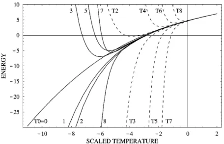
In 3D the picture is much the same, see Fig. 6. The series converge above aT⫽⫺4.5 and diverge below aT⫽⫺5.5.

The nonoptimized series are useful only above aT⫽⫺1.

We define the precision as ( f7⫺ f4)/ f7. f4and f7are the best roots among the sequences. Then we obtain 6.55%,2.94%,0.0247%,0.007 792 22%, at aT⫽⫺5,⫺3,

⫺1.5,⫺1, respectively.

B. Other theories

We compare with other theoretical treatments of the same model. A direct method is the Monte Carlo simulation of the same model. The 2D model was simulated by Moore, Kato, and Nagaosa, and Hu MacDonald. The circles on Fig. 7 for specific heat are the results of the Monte Carlo simulation of TABLE III. Free energy fn at different orders 共a constant

⫺2 log 4␲2_{was subtracted兲.}

aT ⫺2 ⫺1.5 ⫺1 ⫺0.5 f0 ⫺2.194 16 ⫺1.429 41 ⫺0.749 027 ⫺0.146 255 f1 ⫺2.775 16 ⫺1.805 56 ⫺0.988 706 ⫺0.297 222 f3 ⫺2.538 54 ⫺1.682 94 ⫺0.925 643 ⫺0.264 857 f4 ⫺2.558 89 ⫺1.691 43 ⫺0.929 12 ⫺0.266 258 f6 ⫺2.700 76 ⫺1.740 15 ⫺0.945 544 ⫺0.271 734 f7 ⫺2.624 47 ⫺1.718 22 ⫺0.939 384 ⫺0.270 031 f9 ⫺2.515 33 ⫺1.692 3 ⫺0.933 365 ⫺0.268 653 f10 ⫺2.599 43 ⫺1.709 44 ⫺0.936 772 ⫺0.269 318 f12 ⫺2.726 13 ⫺1.731 13 ⫺0.940 395 ⫺0.269 915

TABLE IV. Free energy fnat different orders for 3D.

aT ⫺5 ⫺3 ⫺1.5 ⫺1 f0 ⫺4.733 13 0 2.657 63 3.411 12 f1 ⫺6.493 ⫺0.375 697 2.539 01 3.328 29 f2 ⫺6.925 85 ⫺0.427 383 2.5287 3.3222 f3 ⫺5.275 95 ⫺0.280 923 2.555 51 3.338 f4 ⫺5.680 59 ⫺0.292 936 2.554 55 3.337 57 f5 ⫺4.680 76 ⫺0.265 834 2.556 47 3.338 39 f6 ⫺7.326 54 ⫺0.313 048 2.553 64 3.337 22 f7 ⫺5.331 49 ⫺0.301 797 2.553 92 3.337 31 f8 ⫺8.019 07 ⫺0.316 175 2.553 59 3.3372

the LLL system by Kato and Nagaosa in Ref. 15 performed with 256 vortices. In 3D the model was simulated with 100 vortices by Sasik and Stroud,16magnetization data are com-pared with our results on Fig. 8.

An analytic theory used successfully to fit the magnetiza-tion and the specific heat data29 was developed in Ref. 13. Their free energy density is

feff⫽⫺aT 2 U2 4 ⫹ a_TU 2

冑

U2a_T2 4 ⫹2⫹2 arcsinh

冋

a_TU 2

冑

2

册

, U⫽1 2

冋

1

冑

2⫹ 1

冑

␤A ⫹tanh

冋

aT 4

冑

2⫹ 1 2

册冉

1

冑

2⫺ 1

冑

␤A

冊

册

. 共45兲

The corresponding magnetization and specific heat are shown as dashed lines in Fig. 2 of Ref. 20 and Fig. 7, re-spectively. The theory applies not only to the liquid phase, but also to the solid although the transition is not seen 共should be considered as a 2% effect not determined by the theory兲. At large positive a_T neglecting the exponentially small contributions to U, one obtains

feff⫽⫺aT 2 8 ⫹ aT 2

冑

2

冑

a_T2 8 ⫹2⫹2 arcsinh

冋

aT 4

册

⫽1⫺2 log 2⫹2 log aT⫹ 4 a_T2⫺ 16 a_T4⫹ 320 3a_T6. 共46兲 On the other hand, the high temperature expansion of the optimized Gaussian is ⫺2 log 4␲2_{⫹2 log a} T⫹ 4 a_T2⫺ 18 a_T4⫹ 1324 9a_T6 . 共47兲 One observes that the high temperature expansion of two theories are in remarkable agreement up to the order 1/a_T4.

C. Magnetization, 2D

Experiments on great variety of layered high Tc cuprates 共Bi or Tl5_{based兲 show that in 2D, magnetization curves for} different applied field intersect at a single point ( M*,T*). The range of magnetic fields is surprisingly large共from

sev-FIG. 7. The 2D specific heat. The Monte Carlo data by Kato and Nagaosa in Ref. 15共points兲, specific heat from OPT for n⫽10 共the solid line兲, from phenomenological formula 共the dotted line兲, and Tesanovic et al共Ref. 13兲 theory 共the dashed line兲.

FIG. 8. The 3D magnetization plot. The Monte Carlo data by Sasik and Stroud in Ref. 15 共points兲, specific heat from OPT of different OPE approximants are denoted by numbers. The best ap-proximants are n⫽4,7 共solid line兲.

FIG. 6. The 3D OPT energy and nonopti-mized energy at different orders 共denoted by numbers and ‘‘T’’ plus numbers, respectively兲. One can see clearly OPT series are convergent, for example, at aT⫽⫺5.

eral hundred Oe to several Tesla兲. Assuming this it is easy to derive the scaled LLL magnetization just from the existence of the point. The dimensionless LLL magnetization is de-fined as30

m共aT兲⫽⫺

d feff共aT兲

daT 共48兲

and the measure magnetization is

4␲M⫽⫺ e*h cm_ab

具

兩␺兩 2

_典

_⫽⫺ e*h cm_ab兩␺r兩 2

冉

2␣Tc b

⬘

冊

冑

b␻ 4␲, 共49兲 where␺ is the order parameter of the original model, and␺r

is the rescaled one, which is equal to关d f_eff(a_T)兴/da_T. Thus

4␲M⫽ e*h cmab

冉

2␣Tc b

⬘

冊

冑

b␻ 4␲m共aT兲. 共50兲 Using the definition of aT⫽⫺␩关(1⫺t⫺b)/

冑

bt兴,␩

⫽(2␲2_Gi)⫺1/4_{,b can be written as}

b⫽t

冉

aT 2␩⫾

冑

1⫺t t ⫹ a_T2 4␩2

冊

2 . 共51兲

Thus Eq. 共50兲 implies that

m共aT兲⫽ 4␲cmabM e*h b

⬘

2␣Tc ␩

冑

bt ⫽4␲c␩mabM e*ht b

⬘

2␣Tc 1

冏

冑

1⫺t t ⫹ a_T2 4␩2 ⫾aT 2␩

冏

⫽4␲cmabM␩ e*h兩1⫺t兩 b

⬘

2␣Tc

冏

冑

1⫺t t ⫹ a_T2 4␩2⫾ aT 2␩

冏

. 共52兲 If we assume that the experimental observation that all the magnetization curves intersect at some point (T*, M*),m(aT) is

m共a_T兲⫽C1共a_T⫾

冑

C2⫹a_T2兲, 共53兲

C1⫽2␲cmabM* e*h兩1⫺t*兩 b

⬘

2␣T_c, C2⫽4␩ 21⫺t* t* . On the other hand, if we require that the first two terms of the high temperature expansion of Eq. 共53兲 and the high tem-perature expansion of the magnetization are equal, one finds that

C1⫽14, C2⫽16.

When we plot this line on Fig. 2 of Ref. 20共the dotted line兲 we find that at lower temperatures the magnetization is over-estimated. On the other hand, magnetization of the theory of Tesanovic et al.共the dashed line on Fig. 2 of Ref. 20兲

under-estimate the magnetization. The OPE results are consistent with the data within the precision range until the radius of convergence aT⫽⫺3. It is important to note that deviations

of both the phenomenological formula Eq. 共53兲 and the Te-sanovic’s are clearly beyond our precision range.

We conclude therefore that although the theory of Te-sanovic et al. is very good at high temperatures 共deviations only at the order 1/a_T4) they become of the order 5–10% at aT⫽⫺3. The advantage of this theory is however that it

interpolated smoothly to the solid and never deviates more than 10%. The coincidence of the intersection of all the lines at the same point (T*, M*) cannot be exact. Like in 3D it is just approximate, although the approximation is quite good especially at high magnetic fields.

D. Specific heat, 2D

The specific heat OPE result is compared in Fig. 7 with Monte Carlo simulation of the same model by Kato and Nagaosa15共black circles兲, the phenomenological formula fol-lowing from Eq. 共53兲 共dotted line兲, and the theory of Te-sanovic et al.13共dashed line兲. The agreement with the direct MC simulation is very good.

E. Magnetization in 3D

We compare here our results on the LLL scaled magneti-zation with the Monte Carlo simulation of the LLL system by Sasik and Stroud.16They are actually more precise in 3D. Figure 8 contains several OPE approximants (n ⫽0,1,2,3,4,7,8) and their data on all three magnetic fields 共representing 2T,3T, and 5T in model YBCO兲. According to the criterion of the ‘‘best root’’ the best approximant should be n⫽7. Clearly up to the radius of convergence the agree-ment is within the expected precision.

VI. CONCLUSION

In this paper we obtained the optimized perturbation theory results for both the 2D and the 3D LLL model. It allows to obtain a convergent series共rather than asymptotic兲. The magnetization and specific heat of vortex liquids with definite precision are calculated. On the basis of this one can make several definitive qualitative conclusions. The intersec-tion of the magnetizaintersec-tion lines is only approximate not only in 3D 共the result already observed in Monte Carlo simulation16兲, but also in 2D. The theory by Tesanovic,13 which uses completely different ideas, describes the physics remarkably well in high temperatures and deviates on the 5–10% precision level at aT⫽⫺2 in 2D.

ACKNOWLEDGMENTS

We are grateful to our colleagues A. Knigavko and T. K. Lee for numerous discussions and encouragement and Z. Te-sanovic for explaining his work to one of us and sharing his insight. One of us is grateful to Professor B. Ya. Shapiro and Y. Yeshurun for hospitality at Bar Ilan. The work was sup-ported by NSC of Taiwan grant NSC#89-2112-M-009-039.

*_{Electronic mail: [email protected]}

†_{Electronic mail: [email protected]}

1_{G. Blatter, M.V. Feigel’man, V.B. Geshkenbein, A.I. Larkin, and}

V.M. Vinokur, Rev. Mod. Phys. 66, 1125共1994兲.

2_{D.R. Nelson, Phys. Rev. Lett. 60, 1973共1988兲; E. Brezin, D.R.}

Nelson and A. Thiaville, Phys. Rev. B 31, 7124共1985兲.

3_{E. Zeldov, D. Majer, M. Konczykowski, V.B. Geshkenbein, V.M.}

Vinokur and H. Shtrikman, Nature共London兲 375, 373 共1995兲.

4_{M. Roulin, A. Junod, A. Erb, and E. Walker, J. Low Temp. Phys.}

105, 1099共1996兲; A. Schilling et al., Phys. Rev. Lett. 78, 4833

共1997兲.

5_{R. Jin, A. Schilling, and H.R. Ott, Phys. Rev. B 49, 9218共1994兲;}

P.H. Kes et al., Phys. Rev. Lett. 67, 2383共1991兲; A. Wahl et al., Phys. Rev. B 51, 9123共1995兲.

6_{U. Welp et al., Phys. Rev. Lett. 67, 3563共1991兲.}

7_{D.J. Thouless, Phys. Rev. Lett. 34, 946共1975兲; G.J. Ruggeri and}

D.J. Thouless, J. Phys. F: Met. Phys. 6, 2063共1976兲.

8

G.J. Ruggeri, Phys. Rev. B 20, 3626共1979兲.

9_{N.K. Wilkin and M.A. Moore, Phys. Rev. B 47, 957共1993兲.} 10_{T.J. Newman and M.A. Moore, Phys. Rev. B 54, 6661共1996兲.} 11_{J. Yeo and M.A. Moore, Phys. Rev. Lett. 76, 1142共1996兲; Phys.}

Rev. B 54, 4218共1996兲.

12_{I. Affleck and E. Brezin, Nucl. Phys. B 257, 451 共1985兲; L.}

Radzihovsky, Phys. Rev. Lett. 74, 4722共1995兲.

13_{Z. Tesanovic, L. Xing, L. Bulaevskii, Q. Li, and M. Suenaga,}

Phys. Rev. Lett. 69, 3563 共1992兲; Z. Tesanovic and A.V. An-dreev, Phys. Rev. B 49, 4064共1994兲.

14_{L. Bulaevskii, M. Ledvij, and V.G. Kogan, Phys. Rev. Lett. 68,}

3773共1992兲.

15_{Y. Kato and N. Nagaosa, Phys. Rev. B 48, 7383共1993兲; J. Hu and}

A.H. MacDonald, Phys. Rev. Lett. 71, 432共1993兲; J.A. ONeill and M.A. Moore, Phys. Rev. B 48, 374共1993兲.

16_{R. Sasik and D. Stroud, Phys. Rev. Lett. 75, 2582共1975兲.} 17_{P.W. Stevenson, Phys. Rev. D 23, 2916共1981兲; A. Okopinska,}

ibid. 35, 1835共1987兲.

18

A. Duncan and H.F. Jones, Phys. Rev. D 47, 2560共1993兲; C.M. Bender, A. Duncan, and H.F. Jones, ibid. 49, 4219 共1994兲; B. Bellet, P. Garcia, and A. Neveu, Int. J. Mod. Phys. A 11, 5587

共1996兲; 11, 5607 共1996兲.

19_{H. Kleinert, Path Integrals in Quantum Mechanics, Statistics, and}

Polymer Physics,共World Scientific, Singapore, 1995兲.

20_{D. Li and B. Rosenstein, Phys. Rev. Lett. 86, 3618共2001兲.} 21_{D. Li and B. Rosenstein, Phys. Rev. B 60, 9704共1999兲.} 22_{D.J. Thouless, Phys. Rev. Lett. 34, 946共1975兲; A.J. Bray, Phys.}

Rev. B 9, 4752共1974兲.

23_{R.P. Feynman, Statistical Mechanics 共Benjamin, Reading, MA,}

1972兲.

24_{S. Hikami, A. Fujita, and A.I. Larkin, Phys. Rev. B 44, R10400}

共1991兲; E. Brezin, A. Fujita, and S. Hikami, Phys. Rev. Lett. 65,

1949共1990兲; 65, 2921共E兲 共1990兲.

25_{J. Hu, A.H. MacDonald, and B.D. Mckay, Phys. Rev. B 49, 15263}

共1994兲.

26_{T. Barnes and G.I. Ghandour, Phys. Rev. D 22, 924共1980兲; A.}

Kovner and B. Rosenstein, ibid. 39, 2332 共1989兲; 40, 504

共1989兲.

27_{R. Guida, K. Konishi, and H. Suzuki, Ann. Phys.共N.Y.兲 241, 152}

共1995兲; 249, 109 共1996兲.

28_{R. Seznec, and J. Zinn-Justin, J. Math. Phys. 20, 1398共1979兲.} 29_{S.W. Pierson, O.T. Valls, Z. Tesanovic, and M.A. Lindermann,}

Phys. Rev. B 57, 8622共1998兲; S.W. Pierson and O.T. Valls, ibid. 57, 8143共1998兲; A. Carrington, A.P. Mackenzie, and A. Tyler, ibid. 54, 3788共1996兲.

30 _{Dingping Li and B. Rosenstein, following paper, Phys. Rev. B}