Process versus Product Innovation in Multiproduct Firms
Iordanis Petsas
Department of Economics and Finance, University of Scranton, U.S.A.
Christos Giannikos*
Department of Economics and Finance, Baruch College, U.S.A. &
Columbia University
Abstract
This paper develops a differentiated-goods duopoly model in which firms engage in Cournot-Nash quantity competition. The effects of firm size on the choice of R&D effort between process and product innovation are examined. We find that (a) as firms devote more effort to product innovation, given that they are in the product R&D regime, their incentives to switch from product to process innovation increase, and (b) once the firm is in the process R&D regime, it will perform process R&D indefinitely.
Key words: multiproduct firms; differentiated goods; product innovation; process innovation JEL classification: L10; L25; O31
1. Introduction
There is heterogeneity among firms in the degree of product and process innovation in which they engage. The percentage of total R&D dedicated to different types of innovative activity differs greatly across industries. For example, in petroleum refining, almost three-quarters of total R&D is dedicated to process innovation, whereas less than one-quarter of pharmaceutical R&D is dedicated to process innovation. A large part of such differences is due to differences in exogenous industry-level conditions that systematically differentiate the returns to one sort of innovative activity versus another. Link (1982), for example, finds that
Received May 25, 2005, accepted December 26, 2005.
*Corresponding author: Christos Giannikos, Baruch College, Department of Economics and Finance,
New York, NY 10010, USA (E-mail: Christos_Giannikos@baruch.cuny.edu, Tel: (646) 312-3492). We would like to thank Elias Dinopoulos for valuable comments and suggestions. We would also like to thank David Figlio, Steve Slutsky, and Satyajit Ghosh for useful discussion and suggestions. Final comments from the editor Pao Long Chang and managing editor Jong-Shin Wei helped us improve the exposition of our ideas as we prepared the last draft. Any remaining errors are naturally only our own responsibility. The first author is grateful to the Graduate School of Business, Columbia University and his coauthor for inviting him as a Visiting Scholar during the summer of 2005, a period which has proved instrumental in completing this paper. The second author would like to acknowledge generous research support from Columbia University.
greater product complexity increases the fraction of effort dedicated to process innovation. There is an extensive empirical literature in industrial organization, investigating at the industry level the relationship between firm size and the composition of R&D effort, and hence, the nature of innovation. However, inadequate attention seems to have been paid to modeling these two types of R&D activities and trying to support the empirical papers.
Link (1982) suggests that within industries, firm size, and, thus, across industries, market structure, may also influence the composition of R&D. Scherer (1991) finds that among manufacturing business units considered as a whole, process R&D increases relative to product R&D as the size of the firm increases, with each tenfold increase in business unit sales associated with a highly significant ten point increase in the percentage of R&D expenditures devoted to process innovation.
Cohen and Klepper (1996) propose and test a theory of how firm size conditions the relative amount of process and product innovation undertaken by firms. Their theory explains the close and often proportional relationship within industries between firm size and innovative activity. Their model generates predictions about the relationship between firm size and the share of process R&D. They also test these predictions using patent data that distinguish between process and product innovation and business unit sales data from the Federal Trade Commission’s Line of Business Program. They find that the share of process R&D undertaken by firms indeed rises with firm size within most industries.
One critical question arises about how technologically progressive industries evolve from birth through maturity. When industries are new, there is a lot of entry, firms offer many different versions of the industry’s product, the rate of product innovation is high, and market shares change rapidly. Despite continued market growth, subsequently entry slows, exit overtakes entry, and there is a shakeout in the number of producers, the rate of product innovation, and the diversity of competing versions of the product decline, increasing effort is devoted to improving the production process, and market shares stabilize. This evolutionary pattern has come to be known as the product life cycle (PLC).
While numerous papers have contributed to this description, perhaps the most influential one has been that of Abernathy and Utterback’s (1978). In their paper, they stress that when a product is introduced, there is considerable uncertainty about user preferences and the technological means of satisfying them. As a result, many firms producing different variants of the product enter the market, and competition focuses on product innovation. As users experiment with the alternative versions of the product and producers learn about how to improve the product, opportunities to improve the product are depleted and a de facto product standard, dubbed a dominant design, emerges. Producers who are unable to produce efficiently the dominant design exit, contributing to a shakeout in the number of producers. The depletion of opportunities to improve the product coupled with lock-in of the dominant design leads to a decrease in product innovation. This in turn reduces producers’ fears that investments in the production process will be rendered obsolete
by technological change in the product. Consequently, they increase their attention to the production process and invest more in capital-intensive methods of production, which reinforces the shakeout of producers by increasing the minimum efficient size firm.
Klepper (1996) summarizes regularities concerning how entry, exit, market structure, and innovation vary from the birth of technologically progressive industries through maturity. He develops a model emphasizing differences in firm innovative capabilities and the importance of firm size in appropriating the returns from innovation. His model predicts that over time firms devote more effort to process innovation, but the number of firms and the rate and diversity of product innovation eventually wither.
One of the goals of this paper is to examine these findings (i.e., that within industries the fraction of total R&D a firm devotes to process R&D is an increasing function of the firm’s size) using a differentiated-goods duopoly model in which firms engage in Cournot-Nash quantity competition (in contrast to Klepper’s (1996) model, in which all firms produce a standard product). Firms optimally choose to engage either in product or in process innovation.
Our model differs from those mentioned above in a number of dimensions. First, we consider firms that produce a number of differentiated goods in a duopoly setting and investigate the relationship between firm size and R&D activity based on demand and cost functions. Second, labor is the only primary factor of production: it can be used to produce the differentiated goods and R&D services. R&D services result in discoveries of better production techniques, which enhance the productivity of labor employed in the manufacturing of the differentiated goods. R&D product services result in discoveries of new goods (adding or improving product features).
The analysis generates several insights. For example, an increase in the number of goods produced by a firm and thus an increase in its size (since in our model, the firm size is measured by the firm’s sales and the firm’s sales are proportional to the number of goods produced) causes the firm to perform process R&D regardless of the R&D regime. Given that the firm starts with product R&D, as the number of goods produced increases, the firm’s incentives to switch from product to process innovation increase. Once the firm is in the process R&D regime, it continues to perform process R&D indefinitely. This constitutes a cost-based mechanism that links firm size to the type of R&D activity the firm develops, which is not clear in the models mentioned earlier.
This paper is organized as follows. Section 2 develops the model and shows how it can explain Klepper’s (1996) finding. Section 3 investigates the relationship between firm size and innovative activity in different regimes. Section 4 considers the implications of the analysis for the relationship between firm size and the types of innovative activities undertaken by firms within industries as well as possible extensions of the model. The algebraic details and proofs of propositions in this paper are relegated to Appendix A.
2. A Model of Process versus Product Innovation 2.1 Demand for Differentiated Products
In this section, we develop a model to explain the influence of firm size on the effort devoted to process relative to product innovation. We imagine an identifiable sectoral structure of commodities. Thus, a pencil is a well-defined object and so are a refrigerator, a personal computer, a restaurant meal, and a haircut. Each one of these goods is a differentiated product, however, in the sense that there are many varieties of each available in the market and many more varieties that could potentially be produced. There are red and yellow pencils, soft and hard pencils, white and green refrigerators, 256 MB and 512 MB memory personal computers, and so on.
Since products can be differentiated in many dimensions, one way to introduce preferences for differentiated products is to assume that there are commodities that individuals like to consume in many varieties, so that variety is valued in its own right. The tastes of a representative individual are represented by the following utility function (the economy is able to produce a large number of products, all of which enter symmetrically into demand):
0 1 x D U N i i + =
∑
= α , 0< <α 1, (1)where Di is the per-capita consumption of the th
i product, N is the number of available products and x0 is an outside good (more on this in Dixit and Stiglitz, 1977).
The demand for any individual product i can be derived by solving the following maximization problem:
N D D D1,2...U max subject to , 1 I P D N i i i =
∑
=where Di and Pi indicate the consumption and the price of the
th
i product respectively, and I is the individual’s income. By forming the Lagrangian function (L), the above problem is equivalent to:
⎥ ⎦ ⎤ ⎢ ⎣ ⎡ ⎟ ⎠ ⎞ ⎜ ⎝ ⎛ − − + + =
∑
∑
= = 1 0 0 1 ... , , ,... , 2 1 2 1 max maxL D x I DP x N i i i N i i D D D D D D N N λ α λ ,where λ is the Lagrangian multiplier.
0 0⇔ 1− = = ∂ ∂ − i i i P D D L α α λ , i=1,...,N,
∑
= − = ⇔ = ∂ ∂ N i i iD P I x L 1 * * 0 0 λ , 1 0 0 = ⇔ = ∂ ∂ λ x L .Since λ is fixed, the inverse demand functions for the differentiated goods are: 1 − =α α i i D P , i=1,...,N, (2)
where Di is the per-capita quantity demanded for the th
i product. In monopolistic competition models, λ is taken as fixed because it is assumed that the number of goods produced is large, and thus each firm’s pricing policy has a negligible effect on the marginal utility of income. As the total number of consumers is fixed, we can set the population at 1 without loss of generality. In this case, we do not have to distinguish between total and per capita quantities, so we let Di (i=1,...,N) denote the respective (total or per capita) quantities of the differentiated goods.
2.2 The Duopoly Model
We consider a duopoly in which each firm produces a range of differentiated goods. Good i is produced with the following production function:
ik q
ik L
X =μk
for i=1,...,n1 if k=1 and for i=n1+1,...,N if k=2, (3)
where k denotes firm, Xik denotes the output of good i produced by firm k , and ik
L denotes the amount of labor used in the production of good i by firm k . Thus, production functions are the same for all product varieties within each firm. The number of potential varieties is assumed to be countably infinite, so that only a finite subset of the range is actually produced. The parameter μ ( 1> ) is the quality increment per innovation, whereas the parameters q1 and q2 represent the number of innovations undertaken by firms 1 and 2 respectively (q ∈
{
0,1, 2,....}
). The total number of goods available in the economy is n1+n2=N . Production of eachproduct variety in such an industry is undertaken by only one producer since the other firm can always do better by introducing a new product variety than by sharing in the production of an existing product type.
Using labor as the numeraire, we normalize the wage rate to unity. Then the marginal cost (the cost per unit) of good Xi1 is
1
1μ (q
1
1,...,
i= n ) when firm 1 knows how to produce Xi1 with the q1th process. The marginal cost of Xi2 is
2
1μ (q
2
1,...,
i= n ) when firm 2 knows how to produce Xi2with theq2th process. We assume that both firms produce the quantities demanded of each good.
Since each firm is a multiproduct firm, we measure the firm size by their sales. For example, sales for firm 1 are given by:
nPD D P i n i i =
∑
= 1 1 .This equation implies that the prices are the same for all goods produced within each firm and the quantities produced are the same within each firm. Since the sales of each firm are proportional to the number of goods produced by that firm, we use that number to measure the firm size.
In this section, we consider R&D costs as sunk (i.e., they already have been incurred and are fixed). The profit function for firm 1 for producing n1 goods is as follows:
∑
∑
= = − = 1 1 1 1 1 1 1 n i i q i n i iD D P μ π . (4)In the same way, the profit function for firm 2 for producing n2 goods is given by:
∑
∑
+ = + = − = N n i i q i N n i iD D P 1 1 2 1 2 1 1 μ π . (5)By differentiating equations (4) and (5) with respect to the quantities Di, we obtain the quantities produced of each good, and then we can obtain the value profit functions. Since the value profit functions are symmetric for both firms, we can generalize them and use k to denote either firm (k =1, 2). Simple comparative statics with respect to nk and qk lead to the following two equations and Proposition 1: 0 1 1 ) , ( ) , 1 ( ) 1 ( 1 1 * * * , ⎟⎟ > ⎠ ⎞ ⎜⎜ ⎝ ⎛ ⎟ ⎠ ⎞ ⎜ ⎝ ⎛ − = − + = Δ − − + α α α α μ α α π π π k k k k k k k k q n k n q n q , (6) where * ,nk k π
Δ is the marginal profit of firm k from performing product innovation, and
(
1)
0 1 ) , ( ) , 1 ( (1 ) (1 ) ) 1 ( ) 1 ( * * * , ⎟ − > ⎠ ⎞ ⎜ ⎝ ⎛ − = − + = Δ − − − + α α α α α α μ μ α α π π π k k q k k k k k k k q k q n q n n , (7) where * ,qk k πΔ is the marginal profit of firm k from performing process innovation and where k denotes firm (k =1, 2).
Proposition 1: Total profits for firm k (=1, 2) depend positively on the number of goods produced and the number of process innovations it performs.
Equations (6) and (7) provide a basis for explaining why the firm size tends to increase the marginal returns from process R&D but not the marginal returns from product R&D. In equation (6), the marginal returns to product R&D are independent
of the firm size, whereas in equation (7) the marginal returns to process R&D depend positively on the firm size.
We can now solve explicitly for the number of goods * k
n at which the firm is indifferent between performing one more product R&D and one more process R&D activity. By equalizing equations (6) and (7), we obtain the following proposition.
Proposition 2: If *=
(
1 μ) (
α(α−1)1 μα (1−α)(μα(1−α)−1))
kk q
q k
n , then firm k is indifferent
between performing one more product innovation and performing one more process innovation.
Proposition 2 provides a rationale for Scherer’s (1991) finding that larger firms devote a greater fraction of their R&D to process innovation. The intuition behind this result is straightforward. The marginal returns to process R&D rise with the firm’s size (as it is measured with nk) while the marginal returns to product R&D are constant (independent of nk). If
(
1) (
1 ( 1))
) 1 ( ) 1 ( ) 1 ( *> μqk α α− μαqk −α μα −α − k n , then it
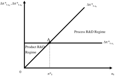
is more profitable for firm k (=1, 2) to switch from product to process innovation. Figure 1 shows the relationship between the marginal profits from process and from product innovation considering the R&D costs as sunk costs. The marginal profit from process innovation is an increasing function of the number of goods produced, while the marginal profit from product innovation is independent of the number of goods produced. Point A in Figure 1 reflects a situation in which the firm is indifferent between performing one more process innovation and one more product innovation. For a small number of goods produced (any point to the left of point A), the firm performs only product R&D. The reason is that when a firm develops a product innovation it reaches new buyers as well as it raises its prices given some degree of transient monopoly power. For a large number of goods produced (any point to the right of point A), the firm performs only process innovation. The reason is that when a firm develops a process innovation it lowers its average cost. Thus, the firm will increase its profits by an amount equal to the reduction in its average cost times the level of output of each good produced. Since, in our model, whenever a firm develops a process innovation, it applies to all goods, the larger the number of goods produced the greater the increase in the firm’s profits.
Next, we consider the case, where firm k is in the product R&D regime (any point to the left of point A in Figure 1). We examine the effect of developing one more product innovation on the incentives to switch from product to process innovation. Firm k is in the product R&D regime if and only if
(
1)
(
( 1) 1)
0 1 (1 ) (1 ) (1 ) ) 1 ( ) 1 ( * , * , − − − < − = Δ − Δ − − − − + α α α α α α α α μ μ μ α α π π k q n k q k n k k k , (8) or *<1(
μα(1−α)−1)
k n .By differentiating equation (8) with respect to nk and after rearranging, we obtain:
(
1)
0 1 ) ( (1 ) ) 1 ( ) 1 ( ) 1 ( * , * , ⎟ − > ⎠ ⎞ ⎜ ⎝ ⎛ − = Δ − Δ Δ − − + − α α α α α α μ α α μ π π k k k k q n n k q k , (9) since μ > 1.Figure 1. Marginal Profits from Process and Product Innovation Considering R&D Costs as Sunk
Proposition 3: Given that firm k (=1, 2) is in the product R&D regime, as each firm produces more goods (develops more product innovations), its incentives to switch from product to process innovations increase.
Proposition 3 explains the relationship between the firm size and the type of innovative activity. The intuition behind this result is straightforward. The returns to process R&D rise proportionally with the firm size while the returns to product R&D are constant with the firm size. Consequently, an increase in the number of goods produced must have a greater positive effect on process than on product R&D, causing the firm to switch from product to process R&D.
3. Model of Product versus Process Innovation Considering R&D Costs
In this section, we examine how firms choose optimally their R&D effort between process and product innovation. We assume for simplicity that firms develop either product or process R&D but not both of them at the same time. There are three regimes: product R&D regime (in the area to the left of point A in Figure 1), process R&D regime (in the area to the right of point A in Figure 1) and neutral R&D regime (point A in Figure 1). Firms start with product R&D due to monopoly power and then they switch to process R&D to exploit economies of scale.
We first examine the decision of the firm to perform one more product innovation or to perform one more process innovation for a given number of goods produced and
k k k,q q , k , * * Δπ π Δ nk
Process R&D Regime
Product R&D Regime 0 n* k k n , k * π Δ k q , k * π Δ A
processes developed given that the firm is in the process R&D regime (any point to the right of point A in Figure 1). This decision is based on the difference between the net marginal profit from product innovations and the net marginal profit from process innovations. Net marginal profit from process innovation includes the R&D costs for process innovation and net marginal profit from product innovation includes the R&D costs for product innovation. If the net marginal profit from process is larger than the net marginal profit from product innovations, then it is more profitable for the firm to switch from product to process innovations.
We assume that firms spend Rp on product R&D and Rc on process R&D. Denote by Rpik the amount spent on product R&D for good i by firm k and by Rck the amount spent on process R&D for all goods by firm k. We assume that process R&D applies to all goods, i.e., it reduces equally the average cost of all goods produced. We further assume that the amount spent on product R&D is the same for all goods produced within the firm. Thus, we arrive at the following proposition.
Proposition 4: If 1( 1) [ ( 1)( ) (1 ) (1 )( (1 ) 1)] ) 1 ( ) 1 ( *= − − − − − − − − + −α αα αα αα α α α μ μ μ pk ck qk k R R n ,
then firm k is indifferent between performing one more product innovation and performing one more process innovation.
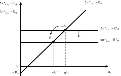
Figure 2 illustrates the net marginal profits from process and from product innovations. At point A, firm k produces *
k
n and is indifferent between performing one more product innovation and performing one more process innovation. Now, by differentiating *
k
n in Proposition 3 with respect to Rpk and Rck, we obtain the next two propositions:
Proposition 5: The number of goods produced by firm k is a decreasing function of its R&D costs from product innovation.
Intuitively, as the firm’s R&D costs from product innovation increase, the net marginal profit from product R&D decreases. Thus, at the original number of goods produced when the firm is indifferent between performing one more product and one more process innovation, the net marginal profit from process innovation is greater than the net marginal profit from product innovation, causing the firm to produce fewer goods.
Figure 3 shows the effect of an increase in the R&D costs from product innovation (Rpk) on
* k
n . When Rpk increases, the net marginal profit from product R&D line shifts down and the equilibrium moves from point A to point B. At point B, the number of goods produced at which the firm is indifferent between developing one more product innovation and developing one more process innovation is less than that of point A ( * *
'
k k
n <n ).
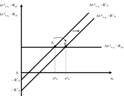
Proposition 6: The number of goods produced by firm k is an increasing function of its R&D costs from process innovation.
As the firm’s R&D costs from process innovation increase, the net marginal profit from process innovation decreases. Thus, at the original number of goods
produced when the firm is indifferent between performing one more product and one more process innovation, the net marginal profit from process innovation is lower than the net marginal profit from product innovation, causing the firm to produce more goods.
Figure 2. Net Marginal Profits from Process and from Product Innovations
Figure 3. Effect of an Increase in R&D Costs from Product Innovation on n∗k
Figure 4 shows the effect of the increase in the R&D costs Rck from process innovation on *
k
n . When Rck increases, the net marginal profit from process innovation shifts to the right and the equilibrium moves from point A to point B. At
ck R − pk n , k R * k− π Δ ck q , k R * k− π Δ nk 0
Process R&D Regime
Product R&D Regime n*k ck q , k R * k− π Δ pk n , k R * k− π Δ ck R − nk pk n , k R * k− π Δ ck q , k R * k− π Δ n*k 0 ck q , k R * k− π Δ A B pk 1 n , k R * k− π Δ pk 2 n , k R * k− π Δ n*k´ A
point B, the number of goods produced when the firm is indifferent between developing one more product innovation and developing one more process innovation is higher than that of point A ( * *
'
k k
n >n ).
Figure 4. Effect of an Increase in R&D Costs from Process Innovation on n∗k
Next, we consider the case, where the firm is at a point to the right of point A in the Figures. In this case, the firm performs only process innovations, since the net marginal profit from process is greater than the nets marginal profit from product innovations in this area.
Firm k is in the process R&D regime if and only if
(
1)
(
(
1)
1)
0 1 (1 ) (1 ) (1 ) ) 1 ( ) 1 ( * , * , − − − > − = Δ − Δ − − − − + α α α α α α α α μ μ μ α α π π q k n k q k n k k k .This last expression implies that 0 ] 1 ) 1 ( [ * μα(1−α)− − > k n . (10)
Suppose the firm has already developed nk product innovations and qk process innovations. Given (nk,qk) and given the fact that the firm is performing only process innovations, we examine if it is more profitable for the firm to develop one more process innovation (qk +1) or to develop one more product innovation (nk+1).
By developing one more process innovation, the difference between the marginal profit from process and the marginal profit from product innovation increases by nk pk n , k R * k− π Δ ck q , k R * k− π Δ 0 n*k A B pk n , k R * k− π Δ ck 1 q , k R * k− π Δ ck 2 q , k R * k− π Δ ck 1 R − ck 2 R − n*k´
(
1)
[
(
1)
1]
1 ) ( (1 ) (1 ) (1 ) ) 1 ( ) 1 ( * , * , ⎟ − − − ⎠ ⎞ ⎜ ⎝ ⎛ − = Δ − Δ Δ − − − − + α α α α α α α α μ μ μ α α π π k q q n k q k n k k k k , (11) where k k k kn q q k ) ( * , * , π π −Δ ΔΔ is the change in the difference between the marginal profit from process and the marginal profit from product innovation due to change in the number of process innovations by one.
If firm k is in the process R&D regime, equation (10) holds and implies that the sign of equation (11) is positive. That is, firm k has an incentive to continue performing process R&D. By developing one more product innovation, the difference between the marginal profit from process and the marginal profit from product innovation increases by
(
1)
0 1 ) ( (1 ) ) 1 ( ) 1 ( ) 1 ( * , * , ⎟ − > ⎠ ⎞ ⎜ ⎝ ⎛ − = Δ − Δ Δ − − + − α α α α α α μ α α μ π π k k k k q n n k q k . (12)The signs of equations (11) and (12) imply Proposition 7.
Proposition 7: Given that firm k (k =1, 2) is in the process R&D regime, it will continue to perform process R&D indefinitely.
This finding suggests that large firms have no incentives to do product R&D, reinforcing the conclusion of earlier studies on R&D effort and firm size (i.e., it supports the idea of R&D costs spreading). The fraction of process R&D versus product R&D rises monotonically with firm size. There is a critical point where the firm enters the process R&D regime and its incentives to remain in this regime are high. Once the firm performs only process R&D, its incentives to switch to product R&D disappear. In a sense, the firm will find it more profitable to find ways to produce its goods cheaper than to create higher quality goods or more variety.
4. Implications and Extensions
The notion that the firm size and the choice between process and product innovation follows a common pattern has become part of the folklore. Our findings support the basic idea that larger firms have an advantage in R&D because of the larger output over which they can apply the results—and thus spread the costs—of their R&D (Cohen and Klepper, 1996). Note, however, that once a firm switches from product to process, it continues to develop only process (since the size of process innovation in our model exceeds 1). If the size of process innovation was small, by performing one more unit of product R&D in the process R&D regime would increase the incentive to switch from process to product innovation. Indeed, if the size of process innovation is less than 1, process innovation is not profitable.
Two limitations of the model need to be brought to the forefront. First, our conclusions depend on and are limited by the functional forms and the assumptions of our model. A different production function, for example, could possibly make the
model conform better to the real world. That is, once a firm is in the process R&D regime, after a critical number of process innovations, it might be possible to switch from process to product innovations.
Second, the assumption that firms will not attend to the production process until product innovation has slowed sufficiently is also restrictive. Yet the history of the automobile industry and others, such as tires and antibiotics, indicates that great improvements were made in the production process well before the emergence of any kind of dominant design. Indeed, many of these improvements were based on human and physical improvements that were not rendered obsolete by subsequent major product innovations. One possible extension of the model is to relax this assumption and explore the implications of this change on the firm’s optimal decision to choose the fraction of process and product innovation. Such a modification to the model would naturally change some of the results, but it would also significantly complicate the analysis.
Appendix A
A. Proofs of Propositions 1, 2, 3, 4, 5, 6, and 7 A.1 Proposition 1
The profit function for firm 1 for producing n1 goods is given by
∑
∑
= = − = 1 1 1 1 1 1 1 n i i q i n i iD D P μ π . (A.1)By substituting equation (2) into equation (A.1), we obtain the following:
) 1 ( 1 1 1 1 i n i q a i D D
∑
= − = μ α π . (A.2)The necessary conditions for a maximum are as follows:
0 ) ( * 1 = ∂ ∂ i i D D π , i=1,...,n1.
These necessary conditions imply that ) 1 ( 1 2 * ( 1 ) 1 − = α μ α q i D , i=1,...,n1, (A.3)
where asterisks denote optimal values. The second-order conditions for a maximum are satisfied and given by
0 ) 1 ( ) ( ( 2) * 2 2 * 1 2 < − = ∂ ∂ α− α α π i i i D D D , i=1,...,n1, (A.4)
since α <1 . The value profits are found by substituting the equations for differentiated goods—i.e., substituting equation (A.3) into equation (A.2):
] ) 1 ( 1 ) 1 ( [ 1( 1) 2 ) 1 ( 1 2 * 1 1 1 1 1 − − = − =
∑
α α α μ α μ μ α α π n q q i q = [( 1 ) (1 )1( 1)( 12 1)] 2 ) 1 ( 1 1 − − − α α α μ α α α q n = ( 1) ( 1)( 1) 1 ) 1 )( 1 ( ) 1 [( 1 − + − − α α α α α α μq n = ( 1) ( 1)( 1) 1 ) 1 ( ) 1 ( 1 + − − − α α α α α α μq n > 0 , (A.5)since α <1. In the same way, the profit function for firm 2 for producing n2 goods, is given by 2 1 1 2 1 1 1 N N i i q i i i n P D D η π μ = + = + =
∑
−∑
= 2 1 1 1 ( ) N i q i i n Dα D α μ = + −∑
.The necessary conditions for a maximum are 0 ) ( * 2 = ∂ ∂ i i D D π , i=n1+1,...,N.
These conditions imply that ) 1 ( 1 2 * ) 1 ( 2 − = α μ α q i D , i=n1+1,...,N.
The second-order conditions for a maximum are satisfied and given by 0 ) 1 ( ) ( 2 *( 2) 2 * 1 2 < − = ∂ ∂ α− α α π i i i D D D , i=n1+1,...,N,
since α < . The maximum profits for firm 2 are 1 0 ) 1 )( 1 ( ( 1) 1 1 2 * 2 2 > − = − − + α α α α μ α α π n q . (A.6)
Since equations (A.5) and (A.6) are symmetric, we generalize them using the following equation: 0 ) 1 )( 1 ( ( 1) 1 1 *= − − > − + α α α α μ α α π k q k k n , (A.7)
for k=1, 2 (where k denotes either firm). Next, we do comparative statics. Since k
n is a discrete variable, we evaluate equation (A.7) at nk and nk+1 for a given qk and then take the difference between them as follows:
0 ) 1 )( 1 ( ) , ( ) , 1 ( ( 1) 1 1 * * * , > − = − + = Δ − − + α α α α μ α α π π π k k k k k k k k q n k n q n q , (A.8) where * ,nk k π
Δ is the marginal profit of firm k from product innovation. Since qkis also a discrete variable, we follow the same procedure as in the above case:
( 1) (1 ) (1 ) * * * , ( 1) ( 1) ( 1) ( 1) 1 1 ( 1, ) ( , ) [ ( ) k ( ) k ] k q q k q k qk nk k q nk k nk nk α α α α α α α α α α π π π μ μ α α + − − + − + − − − Δ = + − = − 0 ) 1 ( ) 1 ( (1 ) (1 ) ) 1 ( ) 1 ( − > − = − − − + α α α α α α μ μ α α qk k n , (A.9) where * ,qk k π
Δ is the marginal profit of firm k from process innovation (k =1, 2). The signs of equations (A.8) and (A.9) prove Proposition 1.
A.2 Proposition 2
By taking the difference between (A.9) and (A.8) and setting it to 0, we obtain the following: 0 ) 1 )( 1 ( ) 1 ( ) 1 ( ( 1) ) 1 ( ) 1 ( ) 1 ( ) 1 ( ) 1 ( ) 1 ( * , * , = − − − − = Δ − Δ − − + − − − + α α α α α α α α α α α μ α μ μ α α π π k k k k q q k n k q k n .
From this equation, we solve for * k n as follows: )] 1 ( 1 [ ) 1 ( ( 1) (1 ) (1 ) *= μqk α α− μαqk −α μα −α − k n . (A.10)
Equation (A.10) proves Proposition 2. Firm k will perform process innovation rather than product innovation if and only if *
, * ,qk knk k π π −Δ Δ > 0. This last expression implies that
(1 ) * ( 1) (1 ) (1 qk) [1 qk ( 1)] k n > μ α α− μα −α μα −α − . (A.10) A.3 Proposition 3
0 ] 1 ) 1 ( [ ) 1 ( 1 (1 ) (1 ) (1 ) ) 1 ( ) 1 ( * , * , − − − < − = Δ − Δ − − − − + α α α α α α α α μ μ μ α α π π q k n k q k n k k k , (A.11) or * k n < 1 (μα(1−α)−1)
. By differentiating equation (A.11) with respect to nk, we obtain the following:
0 ) 1 )( 1 ( ) ( (1 ) ) 1 ( ) 1 ( ) 1 ( * , * , − > − = Δ − Δ Δ − − + − α α α α α α μ α α μ π π k k k k q n n k q k , (A.12)
since μ >1. The sign of equation (A.12) proves Proposition 3.
A.4 Proposition 4
The net marginal profit of firm k from process innovation is given by:
ck q k R n − k − − − − − + ) ( 1) 1 ( (1 ) (1 ) ) 1 ( ) 1 ( α α α α α α μ μ α α . (A.13)
The net marginal profit of firm k from product innovation is given by:
pk qk −R − − − + ) 1 ( 1 1 ) 1 )( 1 ( α α α α μ α α . (A.14)
By equalizing (A.13) and (A.14), we calculate the number of goods * k
n at which firm k is indifferent between performing one more product innovation and performing one more process innovation:
pk q ck q k R R n k k − − = − − − − − + − − − + ) 1 ( 1 1 ) 1 ( ) 1 ( ) 1 ( ) 1 ( ) 1 )( 1 ( ) 1 ( ) 1 ( α α α α α α α α α α μ α α μ μ α α . The last expression implies
(
( ) (1 ) ( 1))
) 1 ( 1 (1 ) ( 1)( 1) (1 ) (1 ) *= μα −α − − αα+ α− − −α μαqk −α μα −α − ck pk k R R n . (A.15)Equation (A.15) proves Proposition 4.
A.5 Proposition 5
By taking the derivative of * k
n in equation (A.15) with respect to the R&D costs Rpk from product innovation, we obtain the following:
0 ) 1 ( ) 1 ( (1 ) (1 ) ) 1 ( ) 1 ( * < − − − = ∂ ∂ − − − + α α α α α α μ μ α α k q pk k R n . (A.16)
Since μ>1 and α <1, both the numerator and the denominator are positive. The sign of the equation (A.16) proves Proposition 5.
A.6 Proposition 6
By taking the derivative of * k
n in equation (A.15) with respect to the R&D costs from process innovation,Rck, we obtain the following:
0 ) 1 ( ) 1 ( (1 ) (1 ) ) 1 ( ) 1 ( * > − − = ∂ ∂ − − − + α α α α α α μ μ α α k q ck k R n . (A.17)
Since μ >1 and α <1, both the numerator and the denominator are positive. The sign of the equation (A.17) proves Proposition 6.
A.7 Proposition 7
First, we calculate the difference between the marginal profit from process innovations and the marginal profit from product innovations as follows:
= Δ − Δ * , * ,qk knk k π π ( 1) ) 1 ( ) 1 ( ) 1 ( ) 1 ( ) 1 ( ) 1 ( ) 1 )( 1 ( ) 1 ( ) 1 ( α+− α− α −α α −α − − α+− α− α α− μ α α μ μ α α k k q q k n ) 1 ( ) 1 ( ) 1 ( ) 1 ( ) 1 ( ) 1 ( ) 1 ( ) 1 ( ) 1 ( ) 1 ( ) 1 ( ) 1 ( ) 1 ( ) 1 ( ) ( ) 1 )( 1 ( ) 1 )( 1 ( ) 1 ( ) 1 ( ) 1 )( 1 ( 1 − − + − − + − − + − − − + − − + − − − − − − − − = + α α α α α α α α α α α α α α α α α α α α μ α α μ α α μ α α μ μ α α μ k k k k q q k q q k n n ] 1 ) 1 ( [ ) 1 ( 1 (1 ) (1 ) (1 ) ) 1 ( ) 1 ( − − − − = − − − − + α α α α α α α α μ μ μ α α k q n k . (A.18)
Since μ >1 and α <1, the sign of equation (A.18) depends on the sign of the expression in the brackets:
] 1 ) 1 ( [ μα(1−α)− − k n .
Firm k is in the process R&D regime if and only if
0 ] 1 ) 1 ( [ ) 1 ( (1 ) (1 ) (1 ) ) 1 ( ) 1 ( * , * , − − − > − = Δ − Δ − − − − + α α α α α α α α μ μ μ α α π π q k n k q k n k k k .
This last expression implies 0 ] 1 ) 1 ( [ * μα(1−α)− − > k n . (A.19)
By developing one more process innovation, the difference between the marginal profit from process and the marginal profit from product innovation increases by:
] 1 ) 1 ( [ ) 1 )( 1 ( ) ( (1 ) (1 ) (1 ) ) 1 ( ) 1 ( * , * , − − − − = Δ − Δ Δ − − − − + α α α α α α α α μ μ μ α α π π k q q n k q k n k k k k , (A.20)
where k k k kn q q k ) ( * , * , π π −Δ Δ
Δ is the change in the difference between the marginal profit from process and the marginal profit from product innovation due to change in the number of process innovations by one. Given that firm k is in the process R&D regime, equation (A.19) holds, which implies that the sign of equation (A.20) is positive. That is, the firm has an incentive to continue to perform process R&D. By developing one more product innovation, the difference between the marginal profit from process and the marginal profit from product innovation increases by:
0 ) 1 )( 1 ( ) ( (1 ) ) 1 ( ) 1 ( ) 1 ( * , * , − > − = Δ − Δ Δ − − + − α α α α α α μ α α μ π π k k k k q n n k q k . (A.21)
The signs of equations (A.20) and (A.21) prove Proposition 7.
References
Abernathy, W. J. and J. M. Utterback, (1978), “Patterns of Industrial Innovation,” Technology Review, 80, 41-47.
Athey, S. and A. Schmutzler, (1995), “Product and Process Flexibility in an Innovative Environment,” RAND Journal of Economics, 26, 557-574.
Cohen, W. M. and S. Klepper, (1996), “Firm Size and the Nature of Innovation within Industries: The Case of Process and Product R&D,” The Review of Economics and Statistics, 78, 232-243.
Dixit, A. and J. E. Stiglitz, (1977), “Monopolistic Competition and Optimum Product Diversity,” American Economic Review, 67, 297-308.
Freeman, C., (1982), The Economics of Industrial Innovation, Cambridge, MA: MIT Press.
Helpman, E. and P. R. Krugman, (1989), Trade Policy and Market Structure, Cambridge, MA: MIT Press.
Klepper, S., (1996), “Entry, Exit, Growth, and Innovation over the Product Life Cycle,” The American Economic Review, 86, 562-583.
Link, A. N., (1982), “A Disaggregated Analysis of Industrial R&D: Product versus Process Innovation,” in The Transfer and Utilization of Technical Knowledge, D. Sahal ed., Lexington, MA: Lexington Books.
Scherer, F. M., (1991) “Changing Perspectives on the Firm Size Problem,” in Innovation and Technological Change: An International Comparison, Z. J. Acs and D. B. Audretsch eds., New York, NY: Harvester Wheatsheaf.