國立交通大學
工業工程與管理學系碩士班
碩士論文
考慮
Gamma 製程變異數發生
變動下之製程能力調整
Capability Adjustment for Gamma Processes
with Variance Change Consideration
研 究 生:古品倫
指導教授:彭文理 博士
考慮
Gamma 製程變異數發生變動下之製程能力調整
Capability Adjustment for Gamma Processes
with Variance Change Consideration
研究生 :古品倫
Student:Pin-Lun Ku
指導教授:彭文理 博士
Advisor:Dr. W. L. Pearn
國 立 交 通 大 學
工 業 工 程 與 管 理 學 系
碩 士 論 文
A ThesisSubmitted to Department of Industrial Engineering and Management College of Management
National Chiao Tung University in partial Fulfillment of the Requirements
for the Degree of Master
in
Industrial Engineering and Management June 2009
Hsinchu, Taiwan, Republic of China
考慮
Gamma 製程變異數發生變動下之製程能力調整
研究生:古品倫
指導教授:彭文理 博士
國立交通大學工業工程與管理學系碩士班
摘要
製程能力指標經常被用來衡量製程製造產品符合規格能力,不僅提供品質保 證的工具,也是提供品質改善方面的一個方針。自從Motorola 公司在 1980 年代 提出6 倍標準差觀念後,許多品質工程師質疑為什麼在計算製程能力之前要增加 1.5 倍標準差的調整。Bothe (2002) 針對此問題,用統計的方法解釋了原因,且 說明調整量是按照抽樣數來決定。在計算製程能力指標之前,需要先假設製程為 穩態的,也就是在生產過程中平均數和標準差不會改變,但是在實務上製程為動 態。當產品品質特性為非常態且變異數未知時,對我們估算製程能力會有什麼影 響?本研究將針對產品品質特性符合Gamma 分配時,其製程變異數改變時之製 程能力調整方法。針對不同的Gamma 參數來計算不同的檢定力,在基於 Bothe 的假設提出修正量。在本研究的最後,我們將利用一個實例來說明當製程品質特 性服從 Gamma 分配並考慮製程變異數發生變動時,應如何調整製程能力指標 pk C 。 關鍵字:Gamma 分配、S2管制圖、製程變動、製程能力指標Capability Adjustment for Gamma Processes with Variance Change Consideration
Student: Pin-Lun Ku
Advisor: Dr. W. L. Pearn
Department of Industrial Engineering and Management
National Chiao Tung University
Abstract
Process capability indices (PCIs) have been proposed in the manufacturing industry to provide numerical measures on process capability, which are effective tools for quality assurance and guidance for process improvement. Motorola, Inc. introduced its Six Sigma quality initiative to the world in the 1980s. Some quality practitioners questioned why Six Sigma advocates claim it is necessary to add a 1.5 shift to the average when estimating process capability. Bothe (2002) provided a statistical reason for including such a shift in the process average that is based on the chart’s subgroup size. When calculating the process capability, we have assumed the process is stable (the process mean and variation do not change), but in practice, the process is dynamic. What is the effect on the capability estimates when the process output has a non-normal distribution with process variance change is remained unknown? This research investigates process capability adjustments when process variance change from Gamma distribution, and compares the detection power of difference parameters and subgroup size from Gamma distributions under Bothe’advises. Finally, we add the adjustment to capability index Cpk of non-normal processes. For illustration purpose, an application example is presented.
Keywords: Gamma distribution, S2 control chart, Dynamic
pk
C , Process
誌謝
兩年時光轉眼間就匆匆過去,想起剛進來交通大學工業工程與管理碩 士班,我還只是個毛頭小子,現在已經做完一篇論文且準備要畢業了。講 起這一篇論文,可以說是我人生中一個重要的轉戾點吧!雖然題目是老師 給定的,但是所有的過程,卻在我生命中留下不可抹滅的記憶。 為什麼這過程是我生命中不可抹滅的記憶呢?因為在這兩年之中,我 學到以前大學沒學到的東西,自己去主動學習、自己主動去找書、主動上 網去找資料,這些種種都是研究所必需學的技巧與謀生方法,以後出社 會,這些就成為你的基礎、做事的態度、以及你永遠伴隨的精神。 當然在這種種的背後,有一雙無私的推手,那就是我的指導教授,彭 文理教授;還有另外一位很重要的學長,黃凱斌學長,它幫助我們論文解 決了很多技術上的問題,很難想像這一篇論文如果沒有他的話會變成怎麼 樣;當然最重要的是要感謝家人,因為他們在後面默默的供給我日常所 需,讓我可以無憂無慮的寫完這一篇論文;不可免俗的感謝所有實驗室的 學長姐,蘇榮弘與巫佳煌及林仲軒學長、雅靜與于庭學姐,及身為同學的 廖律瑋、李佳蕙、蔣宛倫,因為他們給帶來了許多歡樂以及課業上的幫助。 感謝我身旁的所有朋友,謝謝你們的陪伴,我畢業了。Contents
摘要...i Abstract... ii 誌謝... iii Contents... iv List of Tables... v List of Figures ... vi Chapter 1. Introduction... 11.1. Research Background and Motivation ...1
1.2. Research Purpose and Objectives ...2
1.3. Research Organization ...3
Chapter 2. Literature Review...4
2.1. Process Capability Adjustment for Normal Process with Mean Shift...4
2.2. Process Capability Adjustment for Gamma Process with Mean Shift...5
Chapter 3. Introduction to Gamma Distribution ...7
3.1. Gamma Distribution...7
3.2. Statistical Properties of Gamma Distribution ...14
Chapter 4. Process Variance Change Investigation for Gamma Process... 15
4.1. Average Run Length ...15
4.2. Monte-Carlo Simulation for Determining UCL and LCL ...15
4.3. Detection Power of S2 for Gamma Data ...16
4.4. Variance Adjustment for Gamma Process...19
4.5. Capability Adjustment for Gamma Process ...21
Chapter 5. Application ... 23
Chapter 6. Conclusion... 28
References ... 29
Appendix A. AS50 values of Gamma Distributions... 31
List of Tables
Table 1. Probabilities of detecting changes in versus subgroup size. ...5
Table 2. S50 values for several subgroup sizes. ...5
Table 3. AS50 values for several subgroup sizes n and various values. ...6
Table 4. Values of skewness and kurtosis for various Gamma distributions...8
Table 5. Detection power of various from Gamma distributions with n 10. ...18
Table 6. Detection power of various from Gamma distributions with n 15. ....18
Table 7. Detection power of various from Gamma distributions with n 30. ...18
Table 8. AS50 values for several subgroup sizes n and various values. ...200 Table 9. 100 observations are collected from the historical data...24
Table 10. 100 observations are collected from the historical data...25
Table 11. AS50 value for several subgroup sizes n and various (=0.5,1 (1) 10)0 values when . ...310 1 Table 12. AS50 value for several subgroup sizes n and various (=11 (1) 21)0 values when . ...320 1 Table 13. AS50 value for several subgroup sizes n and various (=22 (1) 30)0 values when . ...330 1 Table 14. Average run length of Gamma processes with 1.5 change...34
Table 15. Average run length of Gamma processes with 2 change...35
Table 16. Average run length of Gamma processes with 2.5 change...36
Table 17. Average run length of Gamma processes with 3 change...37
Table 18. Average run length of Gamma processes with 3.5 change...38
List of Figures
Figure 1. Gamma distributions along with normal distributions with same mean and variance, 0 1, 2, 4, 6, 8 and 10, and fixed . ...100 1 Figure 2. Empirical distributions of the sample variance from Gamma and
normal distributions with same mean and variance, =1, 5, 10, 15, 20, and0 30, and fixed . ...110 1 Figure 3. Empirical cumulative distribution functions of the sample variance from
Gamma and normal distributions with same mean and variance, =1, 5,0 10, 15, 20, and 30, and fixed . ...120 1 Figure 4. Empirical distributions of the sample variance with difference Gamma
populations but have same mean. ...13
Figure 5. Probability density function plots for Gamma distribution with different sample sizes...14
Figure 6. Power curves for different subgroup sizes and ...210 Figure 7. Structure of a Backlight module. ...23
Figure 8. Side view of LED ASSY at the backlight module. ...24
Figure 9. Top view of LED ASSY at the backlight module. ...24
Figure 10. Histogram plot of the historical data. ...25
Chapter 1. Introduction
1.1. Research Background and Motivation
Process capability indices (PCIs) are used widely throughout the world to give a quick indication of process capability in a format that is easy to use and understand. During the last decade, numerous process capability indices, including Cp, Cpk, Cpmand Cpmk( Kane (1986), Chan et al. (1988), Pearn et al. (1992)), have been proposed in manufacturing industries to provide numerical measures on process performance. Using process capability indices to express process capability has made the setting and communicating of quality goals much simpler, and their use is expected to continue to increase.
Based on analyzing the PCIs, a production department can trace and improve a poor process so that the quality level can be enhanced and the requirements of the customers can be satisfied. These PCIs have been defined explicitly as
2 2 , min , , , 6 3 3 6 p pk pmUSL LSL USL LSL USL LSL
C C C T
2
2 2 2 min , , 3 3 pmk USL LSL C T T where USL is the upper specification limit, LSL is the lower specification limit, is the process mean, is the process standard deviation, and T is the target value.
The first process capability index Cp considers the overall process
variability relative to the manufacturing tolerance, reflecting product quality consistency. Due to the simplicity of the index, Cp cannot reflect the tendency of process centering and thus gives no indication of the actual process performance. For this reason a more refined index Cpk was developed. The index
pk
C considers process variation and the location of process mean which has been viewed as a yield-based index. But this index fails to measure effectively the effect of process centering on process capability. In fact, it makes no clear distinction between on-target and off-target processes. More importantly, Cpk gives no indication of the direction in which the process is off-target. The Cpm index is based on the idea of the squared error loss, concentrating on measuring the ability of the process to cluster around the target. The Cpm index involves the variation of production items with respect to the target value and the specification limits
that are preset in the factory. The index Cpmk has been constructed by
accounting for the process yield as well as the process loss. This index alerts the user when the process variance increases and the process mean deviates form its target value.
1.2. Research Purpose and Objectives
Ever since Motorola, Inc. introduced its Six-Sigma quality initiative to the world in the 1980s, quality practitioners have questioned why the followers of this initiative have added a 1.5 shift to the process mean when estimating process capability. When asked the reason for such an adjustment, six-sigma advocates claim it is necessary, but offer only personal experiences and three dated empirical studies as justifications (see Bender (1975), Evans (1975), Gilson (1951)). By examining the sensitivity of control charts to detect changes of various magnitudes, Bothe (2002) provided a statistically based reason to this issue. In his study, Bothe assumed that the process data is approximately normally distributed. However, non-normal processes occur frequently in practice. If the process capability indices based on the normal assumption concerning the data are used with non-normal observations, the value of the process capability indices may be incorrect and quite likely misrepresent the actual product quality.
The well-known and usual Shewhart S2 control charts assume that the
observed process data come from a near-normal distribution. However, when the process distribution is unknown or non-normal, the estimator of the parameters for the sampling distribution may not be available theoretically. We use method of moments estimator (MME) to estimate the unknown parameters. Then, we look for S2 control charts under different distributions and use simulation to get
UCL (Upper Control Limits) and LCL (Lower Control Limits).
In this thesis, we show that the detection power performance of S2 control
chart under the Bothe adjustment when the process in control is very sensitive to the assumption of normality. We provide standard deviation change adjustment based on various subgroup sizes and distribution parameters to calculate the estimator of Cpk when data is from Gamma distribution.
Existing literatures focused on treating the problem of capability adjustment with process mean shift but assuming the process variance remained constant. Very few authors have studied the problem of capability adjustment with process variance change. This motivates us to study the issue of capability adjustment for Gamma processes with variance change.
1.3. Research Organization
In this thesis, we introduce the research motivation and purpose in Chapter 1. Secondly, a clear introduction of Bothe’study and adjustment reason are included and adjustment for Gamma processes in Chapter 2. Thirdly, we introduce the Gamma distribution and the statistical properties. In Chapter 4, we use simulation method to find UCL and LCL. Further, we calculate the detection power for various Gamma distributions. We propose the adjustment for standard deviation change under Gamma processes, calling AS , and add the adjustment to50 Cpk
named “dynamic” Cpk. For illustrative purpose, an application is presented in Chapter 5. Finally, we give some conclusions in Chapter 6.
Chapter 2. Literature Review
The process capability adjustment with mean shift for normal and non-normal process had been researched. In this chapter, we will review these papers about adjustments for normal and Gamma processes with mean shift.
2.1. Process Capability Adjustment for Normal Process with Mean Shift
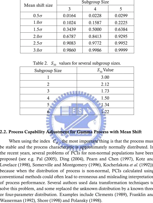
Bothe (2002) advanced a statistical reason why to add a 1.5 shift to the average. Assuming the process approximately normal distribution, control charts can not credibly detect every small movement in process average. So, it is difficult to detect small movements in process. Table 1 presents the probabilities of detecting changes in shift=0.5 (0.5) 3 versus subgroup size with n =3, 4 and 5. When has a small movement and the detection power of Shewhart X control chart is too small to discover. One way to improve the odds of catching small movements in is to increase the subgroup size. In the real world, it is hard to increasing the subgroup size, because it will increase cost. Then, small mean movement affects the PCIs accuracy. However, the probability of nonconformance will increase obviously. For example, when Cpk is 1.33, the probability of nonconformance is 64ppm. If occur 1 shift that will be difficulty detected by control chart, the probability of nonconformance becomes 1350ppm. This amount is almost twenty times more than 64ppm expected by customers from a process having a Cpk reported to be 1.33.
When subgroup size is four and mean shift is 1.5, the detection power will be 0.5. Bothe (2002) considered providing the same detecting power in order to define the several adjustments with different subgroup sizes. He computed many detection powers for different subgroup sizes and showed in Table 1. Table 2 lists shift sizes that have 50 percent chance of remaining undetected, called S50 values,
for subgroup sizes 1 through 6. Mean shift small than S are the ones likely to50
remain undetected (larger moves should be caught by the chart), a conservative approach is to assume that every missed shift is as large as S . And Bothe50
advocated dynamic Cpk be defined as
50 50 50 50 50 50 Dynamic min , 3 3 min , 3 3 3 3 min , 3 3 3 . 3 pk pk LSL S USL S C S S LSL USL S LSL USL S C
Table 1. Probabilities of detecting changes in versus subgroup size. Subgroup Size
Mean shift size
3 4 5 0.5 0.0164 0.0228 0.0299 1.0 0.1024 0.1587 0.2225 1.5 0.3439 0.5000 0.6384 2.0 0.6787 0.8413 0.9295 2.5 0.9083 0.9772 0.9952 3.0 0.9860 0.9986 0.9999
Table 2. S50 values for several subgroup sizes.
Subgroup Size S Value50
1 3.00 2 2.12 3 1.73 4 1.50 5 1.34 6 1.22
2.2. Process Capability Adjustment for Gamma Process with Mean Shift
When using the index Cpk, the most important thing is that the process must be stable and the process characteristic is approximately normally distributed. In the recent years, several problems of PCIs for non-normal populations have been proposed (see e.g. Pal (2005), Ding (2004), Pearn and Chen (1997), Kotz and Lovelace (1998), Somerville and Montgomery (1996), Kocherlakota et al. (1992)), because when the distribution of process is non-normal, PCIs calculated using conventional methods could often lead to erroneous and misleading interpretation of process performance. Several authors used data transformation techniques to solve this problem, and some replaced the unknown distribution by a known three or four-parameter distribution. Examples include Clements (1989), Franklin and Wasserman (1992), Shore (1998) and Polansky (1998).
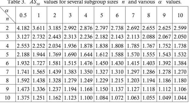
Hsu et al. (2008) provided the process capability adjustment for Gamma process with mean shift. For small process mean shift, the control chart may not detect it and our process capability will be overestimated. Then, they calculated
adjustments which called AS50 with various sample sizes n and Gamma
parameter under Bothe’ advises detection power. Table 3 displays the
magnitude of adjustments AS50 which they provided and data comes from
Table 3. AS50 values for several subgroup sizes n and various values.
Hsu et al. (2008) used the most common method, quantile estimation, to modify PCIs for the non-normal case. Analogous to the normal case, where the “natural” process width is between the 0.135th percentile and the 99.865th
percentile, PCIs can be redefined in terms of their quantiles for possible modification for the non-normal case. The quantile definition for Cpk is defined as 0.99865 0.00135 median median min , . median median pk USL LSL C X X
To investigate the undetected process mean shift, they proposed dynamic
pk
C index for non-normal process as following:
50
50
0.99865 0.00135 median median min , . median median pk USL AS AS LSL C X X By considering an adjustment AS in this assessment to account for50
undetected shifts in process median, the estimate of capability will decrease and the expected total number of nonconforming parts will increase. This nonconforming level assumes that undetected shifts are happening almost constantly and that every one is equal to AS .50
n 0.5 1 2 3 4 5 6 7 8 9 10 2 4.182 3.611 3.185 2.992 2.876 2.797 2.738 2.692 2.655 2.625 2.599 3 3.127 2.732 2.443 2.313 2.236 2.182 2.143 2.113 2.088 2.067 2.050 4 2.553 2.252 2.034 1.936 1.878 1.838 1.808 1.785 1.767 1.752 1.738 5 2.188 1.944 1.769 1.690 1.644 1.612 1.588 1.570 1.555 1.543 1.532 6 1.932 1.727 1.581 1.515 1.476 1.450 1.430 1.415 1.403 1.392 1.384 7 1.741 1.565 1.439 1.383 1.350 1.327 1.310 1.297 1.286 1.278 1.270 8 1.592 1.438 1.328 1.279 1.249 1.229 1.215 1.203 1.194 1.186 1.180 9 1.473 1.336 1.237 1.194 1.168 1.150 1.137 1.127 1.118 1.112 1.106 10 1.375 1.251 1.162 1.123 1.100 1.084 1.072 1.063 1.055 1.049 1.044
Chapter 3. Introduction to Gamma Distribution
In this chapter, we discuss the characteristic of the Gamma distribution, such as its probability density function, mean, and variance. In order to understand the relationships between normal distribution and Gamma distribution, we will compare the third and forth moments of Gamma distribution and standard normal distribution. To further enhance the differences between Gamma and standard normal distributions, we will also compare the two distributions via graphical analysis and observe the changes visually.
Moreover, we will draw the empirical distribution of the sample variance from Gamma distribution such that we can better understand the behaviors of the Gamma distribution and have a more solid foundation for our future studies. Finally, we will discuss the statistical properties of the Gamma distribution, and how it will aids in our future studies.
3.1. Gamma Distribution
In this section, we discuss the property of Gamma distribution. Observations from the Gamma distribution are non-negative. The Gamma distribution can be denoted as Gamma( ) with the probability density function given by0, 0
0 0 0 1 0 0 0 0 1 exp x , 0, 0, 0, f x x x and the mean and variance are given by 2 2
0 0, 0 0
, respectively.
Denote the family of Gamma distributions with mean and variance0 0
0 2 0
by Gamma( ). The Gamma distributions are skewed. To see how this0, 0 distribution is different from the standard normal distribution in terms of
skewness and kurtosis. The skewness of Gamma( ) is0, 0 2 and the0
kurtosis is
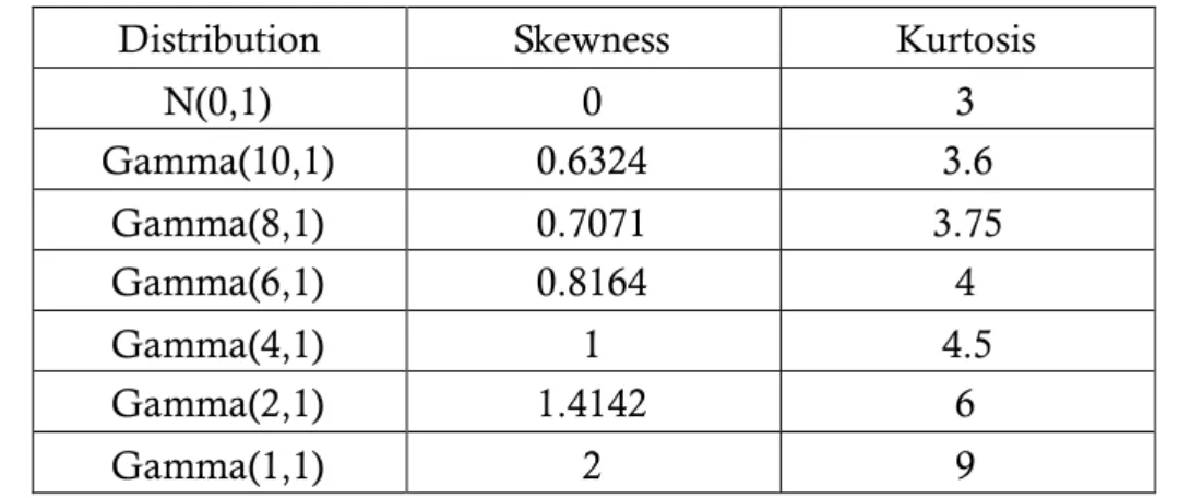
6 . Table 4 presents the values of skewness and kurtosis0 3 (which are defined as the third and fourth moments of the standardized distribution, respectively) of the Gamma distribution and standard normal distribution. We can find that when increasing the values of skewness and0 kurtosis will become small and close to the values of the standard normaldistribution. Whereas, when is decreasing the values of skewness and0
kurtosis will become large and far away the values of the standard normal distribution. From the formula of skewness and kurtosis, we can find that has0 not effect on skewness and kurtosis, no matter how we change the values of ,0 skewness and kurtosis will no difference.
Table 4. Values of skewness and kurtosis for various Gamma distributions.
Distribution Skewness Kurtosis
N(0,1) 0 3 Gamma(10,1) 0.6324 3.6 Gamma(8,1) 0.7071 3.75 Gamma(6,1) 0.8164 4 Gamma(4,1) 1 4.5 Gamma(2,1) 1.4142 6 Gamma(1,1) 2 9
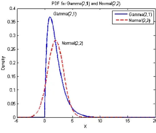
Figure 1 presents several Gamma distributions along with normal distributions with same mean and variance. In this study, we let =1, 2, 4, 6, 8,0
and 10, and fixed . We can be seen from Figure 1, the Gamma distribution0 1
will appears more nearly normal when increases.0
Following the fundamental result regarding normal samples, we have
2 2 1 2 1 n n S where 2S is the sample variance from normal population, and is the2
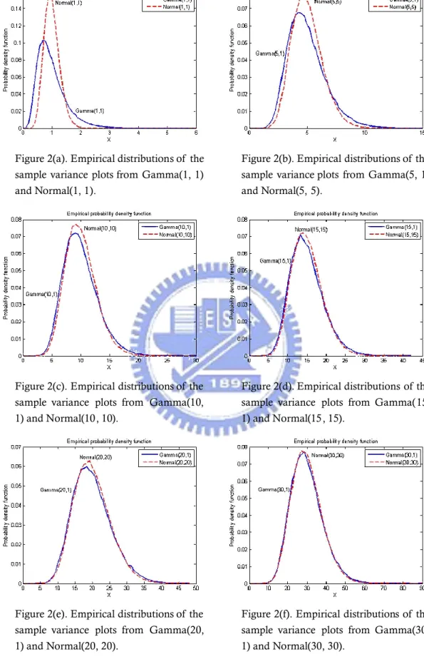
variance of normal distribution. Figure 2 depicts several empirical probability density functions of the sample variance when data come from Gamma and normal populations with same mean and variance. We let =1, 5, 10, 15, 20,0 and 30, and subgroup size is set to be 30. The algorithm is described as following:
Step1: Generate Gamma and normal populations with the same mean and variance.
Step2: Randomly select 30 samples from these two populations to calculate the variance with R replications. (R=1,000,000)
Step3: Draw empirical probability density function plots.
It follows from Figure 1, we see that as increases, the Gamma0
distribution will appear more nearly normal distribution. So, we can infer that the sampling distribution of the sample variance from Gamma distribution appears to be quite close to the sampling distribution of the sample variance from normal population when is large, and this phenomenon can be verified from the0 simulation result shown in Figure 2. Moreover, from Figure 2 we also observe that as is small, the tail will be more elongate (distribution is strongly skewed). In0
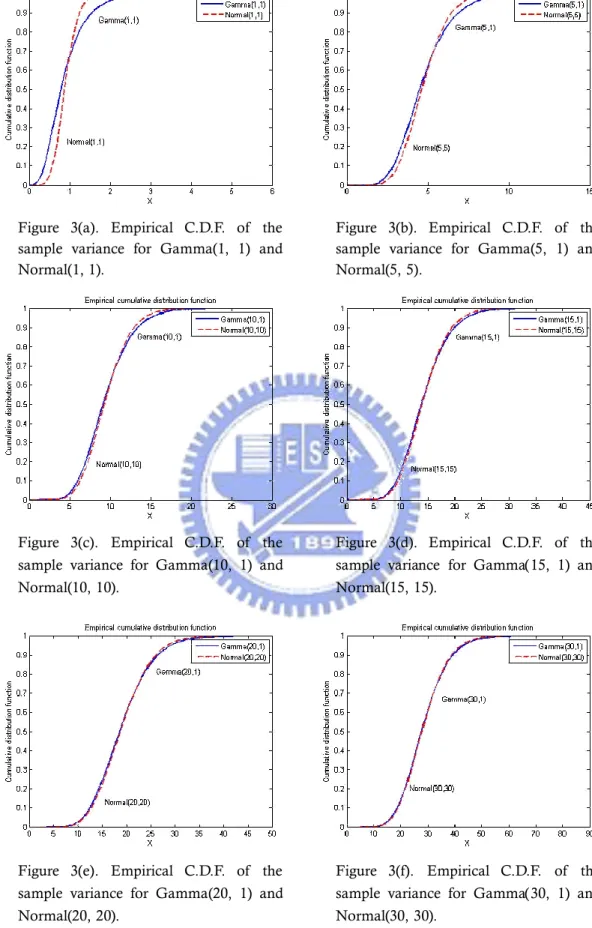
between Figure 2 is that it draws the empirical C.D.F.s of the sample variance with the data.
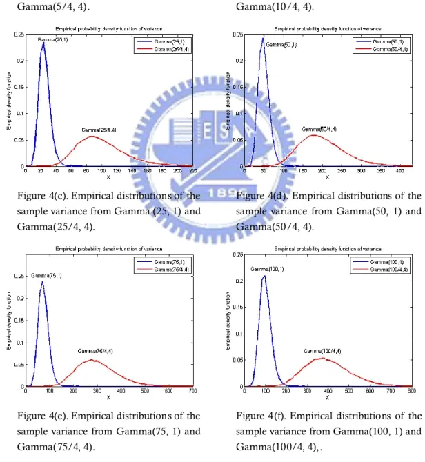
Figure 4 presents many empirical distributions of the sample variance from Gamma population with the same mean but different variance. The algorithm is described as following:
Step1: Generate Gamma distributions with same mean but different variance.
Step2: Random select 30 samples from these two populations to calculate the variance R times. (R=1,000,000)
Step3: Draw empirical C.D.F. plots.
From Figure 4, we can see that when increases the graph will be closer to0 normal sample variance graph. And when is small, the tail will be more0 elongate. Through these discussions above, we wish to study the effects on the capability estimates when the process output has a Gamma distribution with process variance change. We can observe that small has larger variance when0 mean is fixed.
Figure 1(a). Probability density functions for Gamma(1, 1) and Normal(1, 1).
Figure 1(b). Probability density functions for Gamma(2, 1) and Normal(2, 2).
Figure 1(c). Probability density functions for Gamma(4, 1) and Normal(4, 4).
Figure 1(d). Probability density functions for Gamma(6, 1) and Normal(6, 6).
Figure 1(e). Probability density functions for Gamma(8, 1) and Normal(8, 8).
Figure 1(f). Probability density functions for Gamma(10, 1) and Normal(10, 10).
Figure 2(a). Empirical distributions of the sample variance plots from Gamma(1, 1) and Normal(1, 1).
Figure 2(b). Empirical distributions of the sample variance plots from Gamma(5, 1) and Normal(5, 5).
Figure 2(c). Empirical distributions of the sample variance plots from Gamma(10, 1) and Normal(10, 10).
Figure 2(d). Empirical distributions of the sample variance plots from Gamma(15, 1) and Normal(15, 15).
Figure 2(e). Empirical distributions of the sample variance plots from Gamma(20, 1) and Normal(20, 20).
Figure 2(f). Empirical distributions of the sample variance plots from Gamma(30, 1) and Normal(30, 30).
Figure 2. Empirical distributions of the sample variance from Gamma and normal distributions with same mean and variance, =1, 5, 10, 15, 20, and 30,0 and fixed .0 1
Figure 3(a). Empirical C.D.F. of the sample variance for Gamma(1, 1) and Normal(1, 1).
Figure 3(b). Empirical C.D.F. of the sample variance for Gamma(5, 1) and Normal(5, 5).
Figure 3(c). Empirical C.D.F. of the sample variance for Gamma(10, 1) and Normal(10, 10).
Figure 3(d). Empirical C.D.F. of the sample variance for Gamma(15, 1) and Normal(15, 15).
Figure 3(e). Empirical C.D.F. of the sample variance for Gamma(20, 1) and Normal(20, 20).
Figure 3(f). Empirical C.D.F. of the sample variance for Gamma(30, 1) and Normal(30, 30).
Figure 4(a). Empirical distributions of the sample variance from Gamma(5, 1) and Gamma(5/4, 4).
Figure 4(b). Empirical distributions of the sample variance from Gamma(10, 1) and Gamma(10/4, 4).
Figure 4(c). Empirical distributions of the sample variance from Gamma (25, 1) and Gamma(25/4, 4).
Figure 4(d). Empirical distributions of the sample variance from Gamma(50, 1) and Gamma(50/4, 4).
Figure 4(e). Empirical distributions of the sample variance from Gamma(75, 1) and Gamma(75/4, 4).
Figure 4(f). Empirical distributions of the sample variance from Gamma(100, 1) and Gamma(100/4, 4),.
Figure 4. Empirical distributions of the sample variance with difference Gamma populations but have same mean.
3.2. Statistical Properties of Gamma Distribution
The Gamma distribution has a reproductive property: if X and1 X are2
independent random variables and each has a Gamma distribution with possible different values of of1, 2 , but with common value of0 , and with0
0 1 2.
Applying this property, let X X1, 2, , Xn be a sequence of independent distribution of Gamma( ) and then the distribution of0, 0
1 2 n
X X X is Gamma(n ). Using simple statistical technique, we can0, 0 conclude that X
X1 X2 Xn
n ~ Gamma(n ). From Figure 50, 0 nwe observe that for small the variance is larger when mean is fixed.0
Figure 5(a). Probability density function plots for Gamma when 0 ,5 0 ,1 and n .2
Figure 5(b). Probability density function plots for Gamma when 0 ,5 0 ,1 and n .4
Figure 5(c). Probability density function plots for Gamma when 0 ,5 0 ,1 and n .6
Figure 5(d). Probability density function plots for Gamma when 0 ,5 0 ,1 and n .8
Figure 5. Probability density function plots for Gamma distribution with different sample sizes.
Chapter 4. Process Variance Change Investigation for
Gamma Process
In this chapter, we will first discuss the origin of Average Run Length (ARL) and introduce Monte-Carlo method. Then, we use this method to find UCL and
LCL. As mentioned above, we calculate the detection powers under various
Gamma populations. We provide AS50 which modified standard deviation
adjustment for Gamma distribution. Then, adding this adjustment to Cpk named “dynamic” Cpk.
4.1. Average Run Length
Crowder (1987) has studied the ARL of the combined control chart for individuals and moving-range chart. He produced ARL for various setting of the control limits and shifts in the process mean and standard deviation.
ARL is a study of the number of samples required in a process run to detect fault productions. Theoretically, we hope the value of ARL is the smaller, best when it equals to one, because smaller ARL will reduces the loss in production for the detection of faults. However, realistically, ARL will not equal to one in practical application; therefore, we set the value of ARL to be 2 in this study.
From the formula ARL 1 1
, one can deduce , the probability oferroneous judgement to be 0.5. The value , in other words, is the chance of incorrectly judging an incapable process as capable.
4.2. Monte-Carlo Simulation for Determining UCL and LCL
The major purpose of individual control chart can be used to identify shifts or drifts in processes and it is easily to be implemented. But, some assumptions should be satisfied before control charts are used. The assumption include that the process characteristics must be follow normal distribution. Due to
above-mentioned statements, we replace the tradition,
2
22, 1
1 n
S n and
S n2 1
12 2 , 1n, by the quantile of empirical cumulative distribution functionfor different parameters of Gamma( ) to be the upper and lower control0, 0
limits, where 2
/2, 1n
and 1 ( /2), 12 n denote the upper and lower / 2
percentile points of the chi-square distribution with n 1 degrees of the freedom and S2 is an average sample variance obtained from the analysis of preliminary
data.
In order to calculate the probability, one will first need to know the upper and lower control limits (UCL and LCL, respectively) of the process run. Since, to determine the exact form of the sampling distribution for variance is mathematically intractable. In this thesis, Monte-Carlo simulation method was performed to investigate the behavior of sampling distribution for variance with Gamma data and determine the estimated upper and lower control limits.
Hence, in our study, UCL and LCL are estimated through Monte-Carlo simulation method. The steps of Monte-Carlo algorithm to determine the control limits of S2 control chart are summarized as follows:
Step1: Generate random sample X X1, 2, , Xn from Gamma distribution
0, 0
G R times independently, simulating X1i, , Xni G
0, 0
,1, 2, , ; i R (R=1,000,000) Step2: Calculate 2 2 1 1 i n i i j j S X X n
, where i n 1 ji , j X
X n 1, 2, , ; i RStep3: Arrange the simulated observations 2
i
S in increasing order. Denote
2i
S is the ith order statistic as Si2 ; hence, we have
21 22 2R ;
S S S
Step4: Calculate the upper
100
th sample percentile 2 1 R S , where
1 R is the largest integer less than or equal to R
1 . Then 2R1 S is an estimator for 2
1 1 s F .We will utilize the estimator to get lower and upper control limits, and then to obtain the adjustment values.
4.3. Detection Power of S2 for Gamma Data
The main purpose of individual control chart can be used to identify shifts or drifts in process and it is easily to be implemented. In this thesis, we study the effect on the capability estimates when the process output obeys Gamma distribution with process variance change is remained unknown, so the S2
control chart is a convention tool to help us monitor process variability and can help us quickly determine whether the process is stable or not. But, in order to use the S2 control chart, some assumptions should be satisfied, such as the process
characteristics must follow normal distribution. However, due to the search is focus on the Gamma process, violating this assumption, we will need to replace
the traditional upper and lower control limits,
2
22, 1
1 n
S n and
S n2 1
12 2 , 1n , as quantiles of the empirical cumulative distributionfunction from different parameters of Gamma( ).0, 0
Let X X1, 2, , Xn be sequence observations of independent and identically
distribution from Gamma( ). Using the reproductive property of Gamma0, 0
distribution, the mean of the observations is X ( X
nj1X nj ) which isdistributed in Gamma(n ).0, 0 n X and X are distributed from Gammai
Consequently, we can get the power of Gamma process derived from type II error
2 2 2 1 0 2 0.00135 0.99865 1 0 0.99865 0.00135 | | , S S P LCL S UCL K P F S F K G F G F where is the probability of incorrectly judging an incapable process as capable. Hence, the value of 1 is the detection power of Gamma process. GS2
represents the empirical cumulative distribution function of sample variance from Gamma distribution with that standard deviation has changed and is the1
standard deviation after process change ( is the standard deviation of the0
original process). The control limits LCL and UCL are calculated as F0.00135
and F0.99865, respectively.
Since X
X1 X2 Xn
n ~ Gamma(n ), we have0, 0 n0 X Y Gamma n 0,1 n . (1)
So from equation (1), without loss of generality, we can set to find the0 1 detection power.
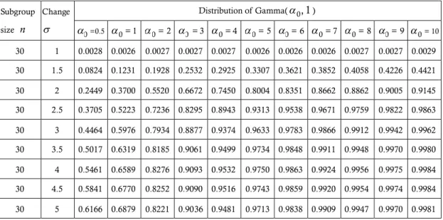
Tables 5-7 below depict the detection powers of the Gamma distribution with the parameters varied from 0 0.5,1 1 10,
0 and subgroup size is 10, 15,1and 30, respectively. The second column on the left is the magnitude of standard deviation change size.
From Tables 5-7, we notice that when increases, the detection power0 also increases accordingly. Moreover, one can see that similar trend exists between the subgroup size and the detection power. Increasing the subgroup size will naturally enhance the probability of identifying the process when it is out of control because more samples are taken into evaluation. Therefore, we should modify the standard deviation adjustments in our study when data come from Gamma distribution.
Table 5. Detection power of various from Gamma distributions with n 10. Distribution of Gamma(0, 1) Subgroup size n Change 0=0.5 0= 1 0= 2 0 = 3 0= 4 0= 5 0= 6 0= 7 0= 8 0= 9 0= 10 10 1 0.0027 0.0027 0.0028 0.0026 0.0027 0.0027 0.0027 0.0027 0.0027 0.0026 0.0027 10 1.5 0.0507 0.0557 0.0690 0.0803 0.0898 0.0983 0.1061 0.1111 0.1153 0.1211 0.1277 10 2 0.1529 0.1686 0.2247 0.2704 0.3102 0.3389 0.3668 0.3865 0.4076 0.4260 0.4400 10 2.5 0.2594 0.2774 0.3504 0.4182 0.4783 0.5267 0.5664 0.5952 0.6212 0.6449 0.6624 10 3 0.3568 0.3610 0.4309 0.5090 0.5740 0.6248 0.6693 0.7029 0.7306 0.7556 0.7781 10 3.5 0.4391 0.4267 0.4807 0.5599 0.6227 0.6765 0.7214 0.7578 0.7899 0.8106 0.8310 10 4 0.5122 0.4836 0.5187 0.5861 0.6484 0.7014 0.7470 0.7813 0.8104 0.8335 0.8559 10 4.5 0.5705 0.5355 0.5527 0.6026 0.6597 0.7114 0.7536 0.7904 0.8198 0.8452 0.8649 10 5 0.6222 0.5791 0.5799 0.6189 0.6689 0.7151 0.7559 0.7905 0.8200 0.8454 0.8655
Table 6. Detection power of various from Gamma distributions with n 15.
Distribution of Gamma(0, 1) Subgroup size n Change 0=0.5 0= 1 0= 2 0 = 3 0= 4 0= 5 0= 6 0= 7 0= 8 0= 9 0= 10 15 1 0.0027 0.0028 0.0027 0.0027 0.0027 0.0027 0.0027 0.0027 0.0027 0.0026 0.0027 15 1.5 0.0569 0.0708 0.0985 0.1183 0.1368 0.1515 0.1634 0.1756 0.1836 0.1925 0.1978 15 2 0.1701 0.2199 0.3136 0.3817 0.4401 0.4885 0.5266 0.5553 0.5828 0.6006 0.6204 15 2.5 0.2775 0.3361 0.4685 0.5644 0.6373 0.6911 0.7346 0.7703 0.7942 0.8140 0.8353 15 3 0.3667 0.4181 0.5503 0.6523 0.7273 0.7844 0.8232 0.8541 0.8785 0.8960 0.9111 15 3.5 0.4408 0.4773 0.5943 0.6937 0.7683 0.8218 0.8599 0.8887 0.9122 0.9276 0.9401 15 4 0.5045 0.5228 0.6204 0.7133 0.7834 0.8356 0.8737 0.9013 0.9227 0.9388 0.9513 15 4.5 0.5591 0.5605 0.6388 0.7237 0.7886 0.8381 0.8772 0.9045 0.9244 0.9423 0.9540 15 5 0.6060 0.5938 0.6537 0.7260 0.7879 0.8365 0.8749 0.9031 0.9248 0.9410 0.9533
Table 7. Detection power of various from Gamma distributions with n 30.
Distribution of Gamma(0, 1) Subgroup size n Change 0=0.5 0= 1 0= 2 0 = 3 0= 4 0= 5 0= 6 0= 7 0= 8 0= 9 0= 10 30 1 0.0028 0.0026 0.0027 0.0027 0.0027 0.0026 0.0026 0.0026 0.0027 0.0027 0.0029 30 1.5 0.0824 0.1231 0.1928 0.2532 0.2925 0.3307 0.3621 0.3852 0.4058 0.4226 0.4421 30 2 0.2449 0.3700 0.5520 0.6672 0.7450 0.8004 0.8351 0.8662 0.8862 0.9005 0.9145 30 2.5 0.3705 0.5223 0.7236 0.8295 0.8943 0.9313 0.9538 0.9671 0.9759 0.9822 0.9863 30 3 0.4464 0.5976 0.7934 0.8877 0.9374 0.9633 0.9783 0.9866 0.9912 0.9942 0.9962 30 3.5 0.5017 0.6319 0.8185 0.9061 0.9499 0.9734 0.9848 0.9911 0.9948 0.9970 0.9980
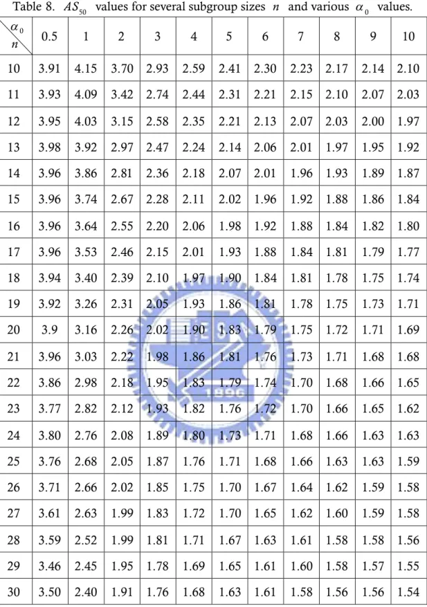
4.4. Variance Adjustment for Gamma Process
The undetected standard deviation change adjustments in Table 8 is called
50
AS which is the magnitude of standard deviation change we need to adjust
based on designated detection power equal 0.5. We find K using this formula
2
1 0
0.5 P LCL S UCL| K
and develop a Matlab program to
compute the standard deviation change adjustment. Table 8 is the standard deviation adjustment under data come from Gamma( ) distribution with0, 1 various parameters of (=0.5 and 1 (1) 10) and n = 10 (1) 30. For example, if0
we set =7 and n =15, then the magnitude of standard deviation change0
adjustment is AS =1.92. We conclude that the standard deviation change50
adjustment of AS =1.92 is required based on the detection power is 0.5 and50
data come from Gamma(7, 1). It can be obviously observed that the adjustment
50
AS get closer to the adjustment under normal population adjustment as 0 increases (see Appendix A.), which is reasonable since the corresponding distribution get closer to the standard normal distribution as increases.0 However, it should be noted that when is small (distribution is strongly0 skewed), the requirement in the capability index formula is much greater than those for normal processes. Utilizing the adjusted process capability formula, the engineers can determine the actual process capability more accurately.
Figure 6 is the plot of power curves. Those lines portray the probabilities of detecting a change in for several given sizes (expressed in units on the horizontal axis). For small changes in , all curves are close to zero. It means the power will be small. From Figure 6(a) we can find that when the change is increased, the power will increase accordingly but not to full 100%. From Figure 6(b) we can find the power will attain to 100% when change as large as possible. The main reason for this phenomenon is that the parameter of Gamma distribution, , is large. The dashed horizontal line drawn on these graphs0
show that there is a 50% probability of missing a 1.84 times the size change in when n is 15, whereas the magnitude of standard deviation change must increase to 2.1 to have the same probability when n is 10. The magnitude of change in that smaller than AS50 are more likely to be missed by a control
chart. Therefore our adjustment AS50 takes into account those changes that are
Table 8. AS50 values for several subgroup sizes n and various values.0 0 n 0.5 1 2 3 4 5 6 7 8 9 10 10 3.91 4.15 3.70 2.93 2.59 2.41 2.30 2.23 2.17 2.14 2.10 11 3.93 4.09 3.42 2.74 2.44 2.31 2.21 2.15 2.10 2.07 2.03 12 3.95 4.03 3.15 2.58 2.35 2.21 2.13 2.07 2.03 2.00 1.97 13 3.98 3.92 2.97 2.47 2.24 2.14 2.06 2.01 1.97 1.95 1.92 14 3.96 3.86 2.81 2.36 2.18 2.07 2.01 1.96 1.93 1.89 1.87 15 3.96 3.74 2.67 2.28 2.11 2.02 1.96 1.92 1.88 1.86 1.84 16 3.96 3.64 2.55 2.20 2.06 1.98 1.92 1.88 1.84 1.82 1.80 17 3.96 3.53 2.46 2.15 2.01 1.93 1.88 1.84 1.81 1.79 1.77 18 3.94 3.40 2.39 2.10 1.97 1.90 1.84 1.81 1.78 1.75 1.74 19 3.92 3.26 2.31 2.05 1.93 1.86 1.81 1.78 1.75 1.73 1.71 20 3.9 3.16 2.26 2.02 1.90 1.83 1.79 1.75 1.72 1.71 1.69 21 3.96 3.03 2.22 1.98 1.86 1.81 1.76 1.73 1.71 1.68 1.68 22 3.86 2.98 2.18 1.95 1.83 1.79 1.74 1.70 1.68 1.66 1.65 23 3.77 2.82 2.12 1.93 1.82 1.76 1.72 1.70 1.66 1.65 1.62 24 3.80 2.76 2.08 1.89 1.80 1.73 1.71 1.68 1.66 1.63 1.63 25 3.76 2.68 2.05 1.87 1.76 1.71 1.68 1.66 1.63 1.63 1.59 26 3.71 2.66 2.02 1.85 1.75 1.70 1.67 1.64 1.62 1.59 1.58 27 3.61 2.63 1.99 1.83 1.72 1.70 1.65 1.62 1.60 1.59 1.58 28 3.59 2.52 1.99 1.81 1.71 1.67 1.63 1.61 1.58 1.58 1.56 29 3.46 2.45 1.95 1.78 1.69 1.65 1.61 1.60 1.58 1.57 1.55 30 3.50 2.40 1.91 1.76 1.68 1.63 1.61 1.58 1.56 1.56 1.54
Figure 6(a). Power curves for subgroup sizes 10 and 15 with 0=10.
Figure 6(b). Power curves for subgroup sizes 10 and 15 with 0= 100.
Figure 6. Power curves for different subgroup sizes and .0
4.5. Capability Adjustment for Gamma Process
The index Cpk has been viewed as a yield-based index since it provides bounds on the process yield for a normally distributed process with a fixed value of Cpk. The proper uses of process capability indices, which are statistical measures of process capability, are based on several assumptions. One of the most essential is that the process monitored is supposed to be stable and the output is approximately normal distribution. When the distribution of a process is non-normal, PCIs calculated using conventional methods could often lead to incorrect and erroneous interpretation of the process capability.
In the recent years, several approaches to the problems of PCIs for the non-normal populations have been proposed. Chen and Pearn (1997) consider come generalizations of these basic capability indices to cover non-normal distribution. In the non-normal case, if we are able to find a better distribution from the data, which provides a very satisfactory fit (this can be tested by means of goodness-of-tests), we can obtain more accurate measures of the three quantiles (X0.00135,X0.5,X0.99865) under consideration, the corresponding Cpu and
pl
C are defined as
0.99865median median
,
upper 0.135% point median median
pu USL USL C X
0.00135 median median .median lower 0.135% point median
pl LSL LSL C X
0.99865 0.00135 median median min , , , median median pk pu pl USL LSL C C C X X where these percentile points can be obtained easily from a simple calculated. Acknowledging that a process will experience changes in process variance of various magnitudes and not all of these will be discovered, we must take them into account when estimating outgoing quality so customers are not disappointed. Because standard deviation changes ranging in size from 0 up to AS50 are the
ones likely to remain undetected (larger changes should be caught by the chart), a conservative approach is to assume that every missed change in process standard deviation is as large as AS .50
Considering the undetected process standard deviation change is as large as
50
AS . Incorporating the adjustments into the Cpk formula we obtained the
“dynamic” Cpk index. When estimating capability, USL minus X0.5
(=median) is divided by AS50 multiple 3 and X0.5 minus LSL is divided
by AS50 multiple 3 where 3 is the estimator for quantile. By making the following modifications:
50 0.99865 50 0.00135 median median min , min , . median median pk pu pl USL LSL C C C AS X AS X By including an adjustment in this assessment for undetected change in standard deviation, the estimate of capability will decrease and the number nonconforming parts measured (calculated) will increase.
Chapter 5. Application
To illustrate how to calculate process capability using “dynamic” Cpk, we consider the following example taken from a LCD production plant. TFT LCD is used widely in television sets, computer monitors, mobile phones and computers, personal digital assistants, navigation systems, projectors, etc. TFT LCD module consists of a color filter substrate, LCD driver, IC chips, backlight module, pixel electrode (ITO), multi-layer PCBs, driving circuits, and chassis assembly. Because liquid-crystal panel can not be luminescing itself, it must rely on backlight module to get display function.
Backlight module is one of the key components in LCD panel. It supplies enough brightness and even light source to let image be displayed. Backlight module consists of CCFL, LED, lampshade, reflector, light guide plate, diffusion sheet, brightness enhancement film, LED ASSY, and iron-frame. Figure 7 shows the structure of backlight module.
Figure 7. Structure of a Backlight module.
When fabricating the backlight module, one of the most important factors that affect the quality of backlight module is the LED ASSY. From Figure 8 and Figure 9 we can discover LED ASSY is extremely thin and connecting with other components. We know that backlight module may easily shut down when it can not connect with other components so the specification of LED ASSY length is very essential. It is one of the most important factors to be considered. The length of the LED ASSY should not fall outside the specification intervals or the customers will not accept the products.
Different models of LCD have different designs, shapes, and production specifications. One characteristic of the LED ASSY which we studied is length. The upper and lower specification limits, USL and LSL, of the length for a particular model of LED ASSY, which we studied, were set to 5.2mm and 0.2mm. The company utilize S2 control chart to monitor the process variance change.
Generally, S2 charts are preferable to their more familiar counterparts, R
charts, when either
1. The sample size n is moderately large, say, n> 10 or 12. 2. The sample size n is variable.
The company use n 15 to monitor the process. Table 9 displays the collected sample data (a total of 100 observations). We use statistica to test the historical data.
Figure 8. Side view of LED ASSY at the backlight module.
Figure 9. Top view of LED ASSY at the backlight module. Table 9. 100 observations are collected from the historical data.
2.4806 1.3633 2.1303 3.2979 3.1802 1.8966 1.5688 1.3464 2.8440 2.5370 2.4708 1.4859 2.1056 3.2820 3.1666 1.8930 1.5691 1.2429 2.8375 2.5061 2.4555 1.5300 2.7667 3.2492 3.1649 1.8867 1.6543 2.4480 2.8229 1.7901 1.2156 1.5443 2.7356 2.9925 3.0897 3.7497 1.6719 2.4170 2.8006 1.7888 1.2005 2.0988 2.6603 2.8731 3.0721 3.7374 1.6772 2.3445 3.4215 1.7869 1.1490 2.0728 1.7036 2.8727 1.9339 3.7294 2.1890 2.3308 3.3219 1.7493 1.1099 2.0508 1.6925 2.8706 1.9273 3.6163 3.5952 1.0401 4.4352 1.7265 2.3021 1.5359 1.6883 1.8627 1.9014 1.7906 3.5020 0.9347 2.0412 2.5430
Variable: length, Distribution: Gamma
Chi-Square test = 4.92138, df = 3 (adjusted) , p = 0.17765
0.5 1.0 1.5 2.0 2.5 3.0 3.5 4.0 4.5 5.0 5.5 6.0 Category 0 5 10 15 20 25 30 35 N o .o f ob se rv at io ns
Figure 10. Histogram plot of the historical data.
Figure 10 displays the histogram plot for the collected data. From goodness-of-tests, we can know the p-value is 0.17765 and we may conclude that the historical data indicates the process pretty approximate to a Gamma distribution (this can be tested by means of goodness-of-fit tests). The parameters
0
and of Gamma distribution could be calculated from historical data0
utilizing method of moments, giving ˆ0 7.97 and ˆ0 0.297.
We utilize this control chart to monitor the process variance, and collect another historical data in Table 10.
Table 10. 100 observations are collected from the historical data.
0.9344 1.2260 2.8183 2.5579 2.9821 1.9371 2.7379 2.3738 2.4632 2.7896 1.1882 1.2760 2.8636 2.5879 1.5828 1.9890 1.6873 2.3918 2.4648 1.8199 1.1927 1.2896 1.2900 3.6060 1.5921 2.9273 1.7042 2.3995 2.5096 1.8349 2.4335 4.2492 2.1425 3.6846 1.5941 1.6168 2.1778 2.9943 2.5129 1.8894 3.0184 1.9990 1.3423 3.7317 2.3328 1.6168 2.2049 1.7349 3.1782 2.0454 3.0676 2.0379 2.1418 1.4496 2.3372 1.6493 2.2517 1.7747 1.7799 2.1315 3.5391 4.0026 1.3266 1.4695 2.3487 2.3058 3.1854 2.6299 1.7800 2.5914 1.9051 2.0261 2.1438 1.5810 3.5000 2.3097 3.2491 2.6641 1.7861 2.5927 1.9102 4.3281 2.1552 3.8022 3.5209 3.1802 3.3434 2.6729 2.7382 3.3624 1.9155 3.7758 3.8512 3.8371 4.3692 4.3704 3.4716 4.7166 2.7836 3.3998
Variable: Var4, Distribution: Gamma
Chi-Square test = 2.93377, df = 4 (adjusted) , p = 0.56897
0.5 1.0 1.5 2.0 2.5 3.0 3.5 4.0 4.5 5.0 5.5 Category 0 5 10 15 20 25 30 N o .o f ob se rv a ti on s
Figure 11. Histogram plot of the historical data.
Figure 11 displays the histogram plot for Table 10. From goodness-of-tests, we can know the p-value is 0.56897 and we may conclude that the historical data indicates the process pretty approximate to a Gamma distribution. The
parameters and0 of Gamma distribution could be calculated from0
historical data utilizing method of moments, giving ˆ0 8.37 and ˆ0 0.296. Therefore, we can use Monte-Carlo method to estimate three quantiles (X0.00135,X0.5,X0.99865) under consideration from this process and get the value as follows:
0.00135 0.26615, 0.5 0.70407, 0.99865 1.67634.
X X X
Then “dynamic” Cpk index can be estimated as follows:
50 0.99865 50 0.00135 median median ˆ min , median median 5.2 0.70407 0.70407 0.2 min , 1.88 1.67634 0.70407 1.88 0.70407 0.26615 0.61, pk USL LSL C AS X AS X with AS 50 1.88 for n 15 form Appendix A. Compared it to the value of the
0.99865 0.00135 median median ˆ min , median median 5.2 0.70407 0.70407 0.2 min , 1.67634 0.70407 0.70407 0.26615 1.15, pk USL LSL C X X
calculated by a traditional capability study (the change of process standard deviation is not considered), we can find that the value of “dynamic” Cpk is much smaller. This result indicates that if the process variance change still not be detected then unadjusted Cpk would overestimate the actual process yield which is not desirable. Our adjustment takes into account those changes that are not detected so that the practitioner would be able to keep its quality promise for this process. As the adjusted process capability drops below the desired quality level, the practitioner should stop the process because the process does not meet his preset capability requirement. The adjustment considered in this thesis should be able to keep its quality promise for this process.
By increasing the subgroup size n , changing in process variance have a higher probability to be detected. For example, if n 30, the AS 50 1.56 for
Gamma distribution then “dynamic” Cpk can be estimated as
50 0.99865 50 0.00135 median median ˆ min , median median 5.2 0.70407 0.70407 0.2 min , 1.56 1.67634 0.70407 1.56 0.70407 0.26615 0.74. pk USL LSL C AS X AS X Increasing n from 15 to 30 will increase the value of dynamic Cpk index from 0.61 to 0.74, and the total number of nonconforming measured (calculated) would be reduced.
Chapter 6. Conclusion
This thesis has considered the problem for adjusting estimate of process capability index by variance change when data is from the Gamma distribution. In the Bothe’study, statistically derived adjustments are proposed under the data assumed to be approximately normal distribution. But the case of non-normal process occurs frequently in practice. We employed the Monte-Carlo simulation method to determine the control limits of S2 control chart and calculated the
variance change adjustment AS50 based on detection power is 0.5 for data comes from Gamma distribution with various values of (=0.5 and 1 (1) 30) and
n =10 (1) 30. For small value of (distribution is strongly skewed), the require
adjustment in the capability index formula is much greater than those for normal processes. Using the adjusted process capability formula, the engineers can determine the actual process capability more accurately. We provided tables for engineers to use for their in-plant applications. A real-world example taken from manufacturing process is investigated to illustrate the applicability of our method. However, this “dynamic” Cpk index assume mean remain stable when variance change. What if mean and variance subjected to undetected increases or decreases? Further studies are needed to determine how those changes would affect estimates of outgoing quality.
References
1. Bender, A. (1975). Statistical Tolerancing as It Relates to Quality Control and the Designer. Automotive Division Newsletter of ASQC.
2. Bothe, D. R. (2002). Statistical reason for the 1.5 shift. Quality Engineering, 14(3), 479-487.
3. Chan, L. K., Cheng, S. W. and Spiring, F. A. (1988). A new measure of
process capability Cpm. Journal of Quality Technology, 20(3), 162-175.
4. Crowder, S. V. (1987). Computation of ARL for combined individual
measurement and moving range charts. Journal of Quality Technology, 19(2), 98-102.
5. Clements, J. A. (1989). Process capability calculations for non-normal
distributions. Quality Progress, 22(9), 95-97.
6. Ding, J. (2004). A method of estimating the process capability index from the first four moments of non-normal data. Quality and Reliability Engineering
International, 20(8), 787-805.
7. Evans, D. H. (1975). Statistical tolerancing: The State of the Art, Part III: Shifts and Drifts. Journal of Quality Technology, 7(2), 72-76.
8. Franklin, L. A. and Wasserman, G. S. (1992). Bootstrap lower confidence limits for capability indices. Journal of Quality Technology, 24(2), 196-210. 9. Gilson, J. (1951). A New approach to engineering tolerances, the machinery
Publishing Co., London, UK.
10. Hsu, Y. C., Pearn, W. L. and Wu, P. C. (2008). Capability adjustment for gamma processes with mean shift consideration in implementing Six Sigma program. European Journal of Operational Research, 191(2), 516-529.
11. Kane, V. E. (1986). Process capability indices. Journal of Quality Technology, 18(1) 41-52.
12. Kocherlakota, S., Kocherlakota, K. and Kirmani, S. N. U. A. (1992). Process capability index under non-normality. International Journal of Mathematical
Statistics, 1(2), 175-210.
13. Kotz, S. and Lovelace, C. R. (1998). Process capability indices in theory and practice, Arnold, London, UK.
14. Pal, S. (2005). Evaluation of non-normal process capability indices using generalized lambda distribution. Quality Engineering, 17, 77-85.
15. Pearn, W. L. and Chen, K. S. (1997). Capability indices for non-normal distributions with an application in electrolytic capacitor manufacturing.
Microelectronics and Reliability, 37(12), 1853-1858.
16. Pearn, W. L., Kotz, S. and Johnson, N. L. (1992). Distributional and inferential properties of process capability indices. Journal of Quality
Technology, 24(4), 216-233.
17. Polansky, A. M. (1998). A smooth nonparametric approach to process capability. Quality and Reliability Engineering International, 14(1), 43-48.
18. Shore, H. (1998). A new approach to analyzing non-normal quality data with application to process capability analysis. International Journal of Production
Research, 36(7), 1917-1933.
19. Somerville, S. E. and Montgomery, D. C. (1996). Process capability indices and non-normal distributions. Quality Engineering, 9(2), 305-316.
Appendix A. AS50 values of Gamma Distributions.
Table 11. AS50 value for several subgroup sizes n and various (=0.5,1 (1) 10)0 values when .0 1 n 0.5 1 2 3 4 5 6 7 8 9 10 10 3.91 4.15 3.70 2.93 2.59 2.41 2.30 2.23 2.17 2.14 2.10 11 3.93 4.09 3.42 2.74 2.44 2.31 2.21 2.15 2.10 2.07 2.03 12 3.95 4.03 3.15 2.58 2.35 2.21 2.13 2.07 2.03 2.00 1.97 13 3.98 3.92 2.97 2.47 2.24 2.14 2.06 2.01 1.97 1.95 1.92 14 3.96 3.86 2.81 2.36 2.18 2.07 2.01 1.96 1.93 1.89 1.87 15 3.96 3.74 2.67 2.28 2.11 2.02 1.96 1.92 1.88 1.86 1.84 16 3.96 3.64 2.55 2.20 2.06 1.98 1.92 1.88 1.84 1.82 1.80 17 3.96 3.53 2.46 2.15 2.01 1.93 1.88 1.84 1.81 1.79 1.77 18 3.94 3.40 2.39 2.10 1.97 1.90 1.84 1.81 1.78 1.75 1.74 19 3.92 3.26 2.31 2.05 1.93 1.86 1.81 1.78 1.75 1.73 1.71 20 3.9 3.16 2.26 2.02 1.90 1.83 1.79 1.75 1.72 1.71 1.69 21 3.96 3.03 2.22 1.98 1.86 1.81 1.76 1.73 1.71 1.68 1.68 22 3.86 2.98 2.18 1.95 1.83 1.79 1.74 1.70 1.68 1.66 1.65 23 3.77 2.82 2.12 1.93 1.82 1.76 1.72 1.70 1.66 1.65 1.62 24 3.80 2.76 2.08 1.89 1.80 1.73 1.71 1.68 1.66 1.63 1.63 25 3.76 2.68 2.05 1.87 1.76 1.71 1.68 1.66 1.63 1.63 1.59 26 3.71 2.66 2.02 1.85 1.75 1.70 1.67 1.64 1.62 1.59 1.58 27 3.61 2.63 1.99 1.83 1.72 1.70 1.65 1.62 1.60 1.59 1.58 28 3.59 2.52 1.99 1.81 1.71 1.67 1.63 1.61 1.58 1.58 1.56 29 3.46 2.45 1.95 1.78 1.69 1.65 1.61 1.60 1.58 1.57 1.55 30 3.50 2.40 1.91 1.76 1.68 1.63 1.61 1.58 1.56 1.56 1.54 0
Table 12. AS50 value for several subgroup sizes n and various (=11 (1) 21)0 values when .0 1 n 11 12 13 14 15 16 17 18 19 20 21 10 2.08 2.07 2.04 2.02 2.01 2.00 1.99 1.98 1.97 1.96 1.95 11 2.01 1.98 1.97 1.96 1.94 1.93 1.92 1.92 1.91 1.90 1.90 12 1.95 1.93 1.92 1.91 1.89 1.89 1.87 1.86 1.86 1.85 1.84 13 1.90 1.88 1.87 1.85 1.84 1.84 1.83 1.82 1.81 1.80 1.80 14 1.85 1.84 1.83 1.82 1.80 1.80 1.79 1.78 1.77 1.77 1.76 15 1.82 1.81 1.78 1.78 1.77 1.76 1.75 1.74 1.74 1.74 1.73 16 1.78 1.77 1.76 1.75 1.74 1.73 1.73 1.71 1.71 1.70 1.70 17 1.75 1.74 1.72 1.72 1.71 1.70 1.70 1.69 1.68 1.68 1.68 18 1.73 1.71 1.70 1.69 1.68 1.68 1.67 1.66 1.66 1.66 1.65 19 1.70 1.69 1.68 1.67 1.66 1.66 1.65 1.64 1.64 1.64 1.63 20 1.68 1.66 1.65 1.65 1.64 1.63 1.63 1.63 1.62 1.62 1.61 21 1.66 1.65 1.63 1.62 1.62 1.63 1.61 1.60 1.59 1.60 1.59 22 1.64 1.62 1.61 1.60 1.59 1.60 1.59 1.59 1.59 1.58 1.58 23 1.62 1.61 1.60 1.59 1.60 1.60 1.58 1.58 1.57 1.57 1.56 24 1.61 1.59 1.59 1.58 1.58 1.57 1.56 1.56 1.55 1.56 1.55 25 1.58 1.58 1.58 1.57 1.56 1.56 1.55 1.54 1.54 1.54 1.53 26 1.58 1.57 1.56 1.55 1.53 1.53 1.53 1.54 1.53 1.52 1.53 27 1.56 1.55 1.55 1.55 1.53 1.53 1.52 1.52 1.52 1.51 1.52 28 1.55 1.55 1.53 1.53 1.53 1.52 1.52 1.51 1.51 1.50 1.50 29 1.54 1.52 1.52 1.52 1.51 1.50 1.50 1.50 1.49 1.49 1.48 30 1.54 1.53 1.52 1.50 1.50 1.50 1.49 1.50 1.48 1.48 1.47 0
Table 13. AS50 value for several subgroup sizes n and various (=22 (1) 30)0 values when .0 1 n 22 23 24 25 26 27 28 29 30 N(0,1) 10 1.95 1.94 1.93 1.93 1.92 1.92 1.92 1.91 1.91 1.80 11 1.89 1.89 1.87 1.87 1.87 1.87 1.86 1.85 1.85 1.76 12 1.83 1.83 1.82 1.82 1.82 1.82 1.81 1.81 1.81 1.72 13 1.79 1.79 1.78 1.78 1.78 1.77 1.78 1.77 1.77 1.68 14 1.76 1.75 1.75 1.75 1.74 1.74 1.74 1.73 1.73 1.65 15 1.72 1.72 1.72 1.72 1.71 1.70 1.70 1.70 1.70 1.63 16 1.70 1.69 1.68 1.68 1.68 1.68 1.68 1.68 1.67 1.60 17 1.67 1.67 1.66 1.66 1.66 1.66 1.65 1.65 1.65 1.58 18 1.65 1.64 1.64 1.64 1.63 1.63 1.63 1.63 1.63 1.56 19 1.63 1.62 1.62 1.62 1.62 1.61 1.61 1.60 1.61 1.54 20 1.61 1.61 1.60 1.60 1.60 1.59 1.59 1.59 1.59 1.53 21 1.58 1.58 1.58 1.58 1.57 1.57 1.57 1.59 1.57 1.51 22 1.58 1.57 1.57 1.56 1.56 1.55 1.55 1.57 1.55 1.50 23 1.56 1.56 1.55 1.55 1.54 1.54 1.55 1.55 1.54 1.49 24 1.55 1.54 1.53 1.54 1.53 1.53 1.52 1.52 1.53 1.48 25 1.52 1.52 1.53 1.53 1.52 1.52 1.51 1.51 1.50 1.47 26 1.53 1.53 1.51 1.51 1.51 1.51 1.50 1.51 1.50 1.46 27 1.51 1.51 1.50 1.51 1.50 1.50 1.49 1.50 1.49 1.45 28 1.49 1.50 1.50 1.50 1.49 1.48 1.48 1.49 1.48 1.44 29 1.48 1.49 1.49 1.48 1.48 1.48 1.47 1.48 1.48 1.43 30 1.48 1.47 1.47 1.47 1.47 1.48 1.47 1.46 1.46 1.42 0
Appendix B. Average Run Length of Gamma Distributions.
Table 14. Average run length of Gamma processes with 1.5 change.
0 n 0.5 1 2 3 4 5 6 7 8 9 10 10 19.67 17.95 14.75 12.85 10.98 10.63 9.68 9.43 8.38 8.11 7.85 11 19.68 17.59 13.09 11.88 9.94 9.64 8.38 7.68 7.46 7.07 6.78 12 18.4 16.46 12.41 11.87 9.05 8.61 7.71 7.21 6.73 6.62 6.42 13 18.39 15.79 11.20 10.18 8.62 7.63 7.17 6.92 6.39 6.20 6.08 14 18.44 14.78 10.60 8.91 7.96 6.97 6.61 6.40 6.05 5.54 5.30 15 16.95 14.47 10.26 8.90 7.35 6.42 6.15 5.94 5.68 5.36 5.07 16 16.81 13.86 9.66 8.27 7.06 6.16 5.63 5.35 4.95 4.83 4.68 17 16.36 11.78 9.79 7.31 6.54 5.93 5.52 4.83 4.59 4.66 4.23 18 16.14 12.87 8.80 6.73 6.17 5.41 4.95 4.76 4.32 4.13 3.92 19 15.42 11.65 8.14 7.03 5.88 5.22 4.73 4.37 3.93 4.01 3.78 20 14.78 10.96 7.69 5.94 5.19 4.60 4.50 4.25 3.78 3.71 3.69 21 15.56 11.61 7.51 6.20 5.15 4.51 4.42 3.76 3.71 3.63 3.58 22 13.86 11.78 7.71 5.58 4.92 4.27 4.04 3.70 3.64 3.47 3.32 23 15.89 10.11 6.79 5.52 4.77 4.06 3.73 3.48 3.29 3.16 2.93 24 14.62 9.83 6.78 5.02 4.45 3.79 3.54 3.38 3.12 3.08 2.85 25 14.07 9.3 6.16 4.90 4.16 3.81 3.52 3.10 3.09 3.02 2.87 26 12.67 9.02 5.83 4.46 4.00 3.47 3.08 2.92 2.86 2.68 2.61 27 12.63 8.93 5.63 4.52 3.72 3.39 3.11 2.88 2.74 2.63 2.60 28 12.83 8.24 5.38 4.09 3.46 3.23 2.97 2.84 2.62 2.60 2.54 29 12.89 8.28 5.32 4.16 3.45 3.16 2.83 2.73 2.58 2.43 2.35 30 11.66 7.85 5.17 4.04 3.63 2.92 2.83 2.59 2.47 2.35 2.30