國 立 交 通 大 學
財 務 金 融 研 究 所
碩 士 論 文
投資人情緒、買賣單不均衡與市場流動性的關係
-以美國ETF市場為例
Sentiment,
Order
Imbalance
and
Liquidity:
Evidence from the ETF Market
研 究 生:張文誠
指導教授:鍾惠民 博士
林建榮 博士
投資人情緒、買賣單不均衡與市場流動性的關係
-以美國ETF市場為例
Sentiment, Order Imbalance and Liquidity: Evidence from
the ETF Market
研 究 生:張文誠
Student : Wen-Cheng Chang
指導教授: 鍾惠民 博士
Advisor : Dr. Hui-Min Chung
林建榮博士 Advisor : Dr. Jane-Raung Lin
國立交通大學
財務金融研究所碩士班
碩士論文
A Thesis
Submitted to Graduate Institute of Finance
National Chiao Tung University
in Partial Fulfillment of the Requirements
for the Degree of
Master of Science
in
Finance
June 2008
Hsinchu, Taiwan, Republic of China
投資人情緒、買賣單不均衡與市場流動性的關係
-以美國ETF市場為例
研究生:張文誠 指導教授:鍾惠民 博士
林建榮 博士
國立交通大學財務金融研究所碩士班
2008 年 6 月
摘要 近年來,行為財務學開始為學者所重視,但主要發展方向為情緒指標與個股報酬 或是市場報酬上的關係,鮮少與市場流動性有關。本文的目的在於找出投資人情 緒指標與市場流動性之間關係。我們分別採用了以市場為基礎的情緒指標和以問 卷調查為主的情緒指標,對兩個假說進行實證。 第一個假說試圖驗證原本 Chordia、Roll 和Subrahmanyam 等學者在2002年提出的流動性模型在加入情緒 指標後,解釋能力會有顯著的增加。結果證實情緒指標在原本的流動性因子之外, 還能對市場報酬有解釋能力,且投資人情緒與市場報酬呈現負向的變動關係。第 二個假說則希望證實情緒指標對市場流動性能有影響力。但實證顯示,情緒指標 對於市場流動性幾乎沒有解釋能力。 關鍵字:投資人情緒、市場流動、市場報酬Sentiment, Order Imbalance and Liquidity: Evidence
from the ETF Market
Student: Wen-Cheng Chang Advisor: Dr. Hui-Min Chung
Advisor: Dr. Jane-Raung Lin
Graduate Institute of Finance
National Chiao Tung University
June 2008
Abstract
This paper is intended to discover the relationship between investor sentiment and market liquidity. Using market-based and survey-based investor sentiment indicators, two hypotheses are tested. The first hypothesis postulates that sentiment indicators have marginal explanatory power to explain market returns beyond the lagged returns and the market liquidity variable, defined as order imbalances. We follow Chordia, Roll and Subrahmanyam (2002) to reconstruct the model by adding sentiment indicators. Consistent with the first hypothesis, the results show that investor sentiment can influence market returns and the relationship between sentiment and market returns is negative. However, the evidence in support of the second hypothesis, which posits that market liquidity variables can be explained by investor sentiment indicators, is not found. As mentioned in previous research, this consequence may be due to the fact that market liquidity can be an investor sentiment indicator.
誌謝 本篇論文能夠完成首先要感謝我的指導教授,鍾惠民博士和林建榮博士。老 師的悉心指導,並在我遇到困難給予幫助,方能有此篇論文的產生。同時也感謝 論文口試委員,陳煒朋博士、何耕宇博士與李漢星博士對於本篇論文的寶貴意 見。 在寫論文的過程中,難免遇到困難。很感謝博班的淑芳學姐在我對論文題目 毫無頭緒時給我的指點與做論文過程中給我的建議,以及敬貿學長在我對資料處 理流程不明白的地方多所指導。也很感謝我的室友們,建佑和政岳,總是在我資 料處理有困難或是思路不通時幫助我,並陪伴我一起度過做論文時的不順遂。平 常常在一起吃飯的以文、詩政和渝薇也常陪我聊天解悶並給予我鼓勵。也很感謝 小田在我程式遇到困難時,義不容辭的拔刀相助,和最後幫我順稿的大熊。也謝 謝電子所的東祐在我找不到人幫忙寫程式時,很熱心的伸出援手,以及資工所的 菘瑋在程式上的協助。還有蓓華在我求助無門時,願意幫我跟對方溝通幾句,雖 然妳的努力最後仍是無用。 最後,要感謝我的家人總是能在我論文不順時包容我,並在背後支持著我。 如果沒有你們,或許就沒有現在的我,願將我的一切成就歸於我的家人。 文誠 謹誌於新竹交通大學 中華民國九十七年六月
Contents
1. INTRODUCTION AND MOTIVATION ... 1
2. LITERATURE REVIEW ... 3
2.1SENTIMENT AND MARKET RETURNS ... 3
2.2SENTIMENT BETA AND HARD-TO-VALUE,DIFFICULT-TO-ARBITRAGE HYPOTHESIS (HV-DA) ... 5
2.3MARKET LIQUIDITY AND MARKET RETURNS ... 7
3. RESEARCH METHODOLOGY ... 9
3.1DATA ... 9
3.2VARIABLES ... 10
3.3METHODOLOGY ... 12
3.4HYPOTHESES AND MODELS ... 14
4. EMPIRICAL RESULTS ... 17
4.1RETURNS,ORDER IMBALANCES, AND INVESTOR SENTIMENT ... 17
4.2LIQUIDITY MODEL WITH SENTIMENT ... 20
5. CONCLUSIONS ... 24
REFERENCES ... 26
List of Tables
TABLE 1 SUMMARY STATISTICS FOR EQUATION 1 ... 33 TABLE 2 THE ESTIMATE EMPIRICAL RESULTS OF EQUATION 1... 37 TABLE 3 DESCRIPTIVE STATISTICS FOR EQUATIONS 2 AND 3 ... 38 TABLE 4 PEARSON CORRELATIONS MATRIX FOR EQUATIONS 2 AND 3 ... 40 TABLE 5 THE EMPIRICAL RESULTS FOR EQUATIONS 2 AND 3 ... 44
1. Introduction and Motivation
Efficient market hypothesis (EMH) is an important theory in traditional finance. It argues that investors are rational and stock prices will reflect all market-related information. As a result, a temporary price divergence will revert to the theoretical price because of arbitrage behavior. Price divergence is an impermanent phenomenon. The so-called efficient capital market means that security prices reflect all the available information completely and accurately. Broadly speaking, it is impossible for investors to obtain abnormal returns. Namely, investors cannot continuously defeat the stock market.
However, scholars have begun to challenge this almost irrefutable theory because of a number of unexplained market anomalies, such as the January effect, the weekend effect, and the emergence of the huge volatility in the stock market. Thus, the topic of behavioral finance based on psychology has begun to flourish in the past decades. Scholars have tried to explain every kind of capital market phenomenon from the view point of investors. In addition, behavior finance scholars consider that limits of arbitrage exist.1 This thinking results from the belief of betting against sentiment investors being costly and risky.
There are many kinds of investor sentiment indicators. In order to predict and expound on the movement of the capital market, experts and scholars endeavor to find these indicators which are like technical indicators. In this article, we use both market-based and survey-based investor sentiment indicators as our measure of sentiment.
Market liquidity is measured by the aggregate daily order imbalance, which is measured by buy orders less sell orders, i.e. the net-buying pressure, and the
1
percentage spread. Excess buy or sell orders reduce liquidity. When the market declines, the order imbalance will increase, and vice versa. This reveals that investors are contrarians.
In this article, we intend to find the interactions among liquidity, investor sentiment and market returns. We choose two ETFs, which are the S&P 500 ETF (SPDR) and the NASDAQ 100 ETF (QQQQ), as our study targets because they can represent the whole market performance.
A growing number of previous studies suggest that liquidity predicts stock returns. Baker and Stein (2004) verify that the predictive power of aggregate liquidity is huge. They also propose a theoretical model to explain the following. Additionally, the market makers are considerably concerned about market liquidity. When market liquidity is not sufficient, they have the obligation to offerquotes to increase liquidity. Thus, we attempt to discover which factors will affect market liquidity and how the explanatory power will change if investor sentiment indicators are added into the liquidity model. We believe our study is helpful for market makers and financial authorities in understanding market conditions.
We discuss two important differences from previous articles in our paper. First, while previous studies on investor sentiment mainly focus on its impact on market returns, this paper intends to discover the relationship between investor sentiment and market liquidity by considering not only the effects on the percentage spread but also the effects on net-buying pressure. To the best of our knowledge, there are no previous studies which have investigated this issue. Second, unlike most previous literature using principle component analysis as a means of extracting composite investor sentiment measures, we follow the method of Simon and Wiggins (2001) to directly employ sentiment indicators. They consider that this method can reserve most of the important information in the sentiment indicators.
This paper endeavors to contribute to the understanding of sentiment factors and trading activities; particularly, that the research design will investigate the relationship between the sentiment factor and the market liquidity supply. We examine the effects of sentiment factors on market liquidity via the amended sentiment-adding liquidity model. Having understood the relationship between investor sentiment indicators and market liquidity, this paper can help the authorities and market makers grasp conditions of market liquidity in order to develop their market functions.
This thesis finds the negative and significant relationship between investor sentiment indicators and market returns. However, investor sentiment indicators have no explanatory power on market liquidity. Investor sentiment indicators may be excellent predicting indicators for market returns, but not for market liquidity.
The remainder of this paper is organized as follows. Section 2 summarizes the related literature about the relations between investor sentiment, market liquidity and returns. Section 3 describes the data, two hypotheses and the research methodology. Section 4 discusses the statistical digitals and the empirical results of the models. Conclusions are provided in section 5.
2. Literature Review
2.1 Sentiment and Market Returns
In the classical financial theory, investor sentiment does not play a role in the cross-section of stock prices, realized returns, or expected returns. For instance, in the traditional CAPM (Capital Asset Pricing Model) theory, the only explanatory factor for asset returns is systematic risk, which is measured by asset beta timing the market risk premium. The more systematic risk investors assume, the more returns investors
obtain. The relationship between asset returns and systematic risk is positive. Baker and Wurgler (2007), however, challenge this point of view. They consider that even if speculative and hard-to-arbitrage securities have higher beta value, according to their theoretical diagram, these securities should have lower returns.
Baker and Wurgler (2006) also find that when beginning-of-period sentiment indicators are low, subsequent returns are relatively high for stocks with the following qualities: small, young, high volatility, unprofitable, non-dividend-paying, extreme growth, and distressed. When sentiment indicators are high, these categories of stocks earn relatively low subsequent returns. This finding is consistent with their prediction that investor sentiment has a large effect on securities whose valuations are highly subjective and difficult to arbitrage. In addition, several firm characteristics display no unconditional forecasting power originally, but those characteristics hide strong conditional patterns that become visible only after conditioning on sentiment.
Although investor sentiment indicators have been widely used, a small ropotion of literature have focused on their efficacy. Clarke and Statman (1998) find that the Bullish Sentiment Index, which is a survey-based measure of the bullishness of newsletter writers, does not have significant predictive power for S&P returns. Brown and Cliff (1999) find that survey measures of sentiment are driven largely by lagged returns. They also find that their composite sentiment measures produced by using the principle component analysis method have predictive power for subsequent returns at 2-year and 3-year horizon and for deviations of stock prices.
Simon and Wiggins (2001) investigate the predictive power of market-based sentiment measures such as VIX (Volatility index), put-call ratio, and TRIN for subsequent returns on the S&P 500 futures contract over 10-day, 20-day, and 30-day horizons from January 1989 through June 1999. They find that these three sentiment measures generally have both statistical and economic forecasting power for
subsequent S&P 500 futures over the sample period of January 1989 through June 1999. They also use stimulation to find evidence that greater returns and risk-adjusted returns will have been earned from buying the S&P 500 futures when the sentiment indicators are flashing a high versus low level of fear.
Unlike previous articles from authors such as Baker and Wurgler (2006 and 2007), and Brown and Cliff (1999), which used principal component analysis to extract composite sentiment indicators, we adopt a method like the one proposed by Simon and Wiggins (2001) to directly examine the forecasting power of sentiment indicators. The method is used because it can preserve the information included in the investor sentiment measures. We also use the market-based sentiment measures such as VIX, VXN and put-call ratio, and survey-based sentiment measures such as AAII in our empirical studies.
2.2 Sentiment Beta and Hard-to-value, Difficult-to-arbitrage Hypothesis (HV-DA)
Glushkov (2006) uses sentiment beta to measure investor sentiment. The definition of sentiment beta is the sensitivity of returns to sentiment. He tests two hypotheses in his paper. The first hypothesis is the so-called HV-DA hypothesis. This postulates that the stocks of some firms are more easily affected by investor sentiment because of the differences in firm characteristics. He finds that more sensitive stocks are smaller, younger, with great short-sales constraints, higher idiosyncratic volatility and lower dividend yields, and this result is consistent with Baker and Wurgler (2006 and 2007). The second hypothesis predicts that stocks which are more sensitive to the movement in investor sentiment are more likely to be held by individual investors. Evidence supporting the second hypothesis is mixed: institution investors got rid of stocks with high sentiment sensitivity throughout the 1980‘s, but held more of these
stocks throughout the 1990‘s.
The HV-DA hypothesis states that some stocks are more affected by irrational investor sentiment than others because of differences in their characteristics. For some younger growth stocks with short earning history and no dividends, it is hard to use the discount cash flow (DCF) model to evaluate their present value. This means that investor individual judgment plays a vital role when deciding the present value of those stocks. Therefore, hard-to-value stocks may be more sensitive to the fluctuation of investor sentiment. On the other hand, small stocks may be more sensitive to sentiment because they are difficult to short sell (Jones and Lamont (2002), D‘Avolio (2002)). Even if short selling is allowed, it is still difficult and costly for arbitragers to maintain a short position for a period of time. Because hard-to-value stocks are more sensitive to the fluctuation of sentiment, astute investors will lose their interest in the arbitrage of these kinds of stocks. This noise trader risk (De Long et al. (1990)) makes hard-to-value stocks also difficult-to-arbitrage. Thus, given the arbitrage limits and risks that arbitragers encounter, sentiment investors may exert their significant influence over the prices of stocks which are smaller, younger and volatile, and make them more vulnerable to sentiment change.
There are several new findings not documented in Baker and Wurgler (2006). First, evidence shows that age, the firm‘s dividend policy and growth potential have explanatory power on relative sentiment sensitivities. Second, after controlling size and volatility, growth stocks are more sensitive to sentiment than distressed stocks.
As mentioned above in the two subsections, those articles discuss cross-section stock market returns. Our paper, however, is about time-series market returns. That is because our paper maintains the focus on the relationship among market liquidity, market returns and sentiment indicators. This is another big difference between our paper and previous literature concerning investor sentiment.
2.3 Market Liquidity and Market Returns
Order imbalance is one indicator to represent market liquidity. Most existing literature analyzing order imbalance is about specific events. For example, Lauterbach and Ben-Zion (1993) examines the behavior of the small market during the October 1987 crash. Blume et al. (1989) analyze order imbalances and stock price movements around the October 1987. Fung (2007) discovers the interactions between the arbitrage spread and order imbalances. Hasbrouck and Seppi (2001) find out common factors in returns, order flow, and market liquidity for thirty Dow Jones stocks during 1994. Brown et al. (1997) study the relationship between order imbalances and stock returns in the Australian stock market over one and two years, respectively.
There are also a growing number of studies suggesting that market liquidity predicts stock returns, both at the firm level and in the time series of the aggregate market. Amihud and Mendelson (1986) find that bid-ask spread is a factor to explain expected returns. Brennan and Subrahmanyam (1996) investigate that the relation between required rate of returns and the measure of liquidity. Jones (2002) suggests that time-series variation in aggregate liquidity is an important determinant of conditional expected stock market returns.
Furthermore, Chordia et al. (2001) argue that equity market returns and recent market volatility affect liquidity and trading activity. And they also find some factors which influence liquidity and trading activity. Those factors include short- and long- term interest rates, default spreads, market volatility, recent market movements, and indicator variables for the day of the week, for holiday effects, and for major macroeconomic announcements.
Backer and Stein (2004) establish a model to explain why increase in liquidity forecasts lower subsequent returns. They also discuss the relationship between market
liquidity and investor sentiment in their model. The most important conclusion in their paper is that market liquidity can be an investor sentiment indicator in the market with short-sale constraints.
Chordia et al. (2002) try to discover the tripartite association among trading activity, liquidity, and stock market returns. They have several important empirical results.
Firstly, order imbalances are strongly related to past market returns. Investors behave like contrarians, namely they buy after market declines and sell after market advances. This behavior is more apparent when the market declines.
Secondly, strong contemporaneous association exists between changes in the absolute level of market-wide order imbalance and market-wide liquidity. The relationship between order imbalances and market liquidity may arise when specialists cannot adjust the quotes on both sides of the market during the period of large order imbalance. Although order imbalance appears to have no forecasting ability, evidences reveal that both the number of trades and the market returns can forecast future changes in liquidity. A bear market predicts lower market liquidity the next day, and a bull market predicts higher market liquidity the next day. This consequence is consistent with inventory models of liquidity proposed by Stoll (1978a).
Thirdly, stock returns are strongly and contemporaneously related to order imbalances. Evidence shows that market prices tend to reverse following declines and continue to follow previous up moves. There is also evidence that returns are predictable using past imbalances and past returns following large-negative-imbalance, large-negative-return days, but there is no forecasting power following high-positive-imbalance, high-positive-return days. Therefore, as mentioned above, the results reveal that order imbalances influence market liquidity and market returns.
This result is consistent with Kraus and Stoll (1972a, b), in which large sales are followed by reversals but large buys are not.
Fourthly, there is strong relationship between order imbalances and contemporaneous absolute returns after controlling for market volume and market liquidity.
3. Research Methodology
3.1 Data
This study employs intra-day ETF trading and quoting data taken from the NYSE Trade and Quote (TAQ) database. The period under examination is from 1 January 1995 to 31 December 2003 because this period of time covers an industry cycle of the dotcom bubble. The exchanges we chosen are Amex (American Stock Exchange), NYSE (New York Stock Exchange), NASDAQ (National Association of Securities Dealers Automated Quotation System), and INSTINET. The ETF traded price and traded volume sources are the Datastream database and the website of Yahoo Finance. All investor sentiment indicators come from internet websites, such as CBOE (VIX, VXN and put-call ratio) and American Association (AAII).
Spider, also called the Standard & Poor's Depositary Receipt (SPDR) is the abbreviation of an exchange-traded fund (ETF) that tracks the S&P 500 Index. It trades on NYSE, and its trading symbol is SPY. The trade of SPY has begun trading in 1993. Each share of a spider trades one-tenth of the dollar-value of the S&P 500 index. Spider, which is traded like stocks, can be short sold, be bought on margin, provide dividend payments and incur regular brokerage commissions when traded. Spider has the largest market value in the world.
The Nasdaq-100 Trust (QQQQ) may be the best-known ETF in existence. It tracks the Nasdaq-100 Trust Index, which comprises 100 of the largest companies traded on the Nasdaq stock exchange. QQQQ has begun trading in 1999. Each share of a QQQQ trades one-fortieth of the value of the Nasdaq 100 index. Because market investors‘ focus is on the high-tech stocks, QQQQ becomes the favorite of the high-tech stocks investors. QQQQ is the ETF with the highest liquidity in the world.
The reason we choose ETF as our variables is because they can represent the trading condition of the entire market. In particular, QQQQ tracks the Nasdaq-100 index, so it is closer to the characteristics of smaller, younger, and high volatility stocks, which are also more sensitive to investor sentiment. Therefore, we choose Spider and QQQQ as our market returns variables.
3.2 Variables
In this section, we introduce four investor sentiment indicators—VIX, VXN, put-call ratio, and AAII, and two liquidity indicators—percentage spread and net buying pressure (order imbalance) used in our regression.
VIX, computed from Black-Scholes model, was implied volatilities of S&P 100 index options which are traded in the CBOE. The options used in the calculation were the closest in-the money and out-of-money calls and puts of the two front month contracts. These eight implied volatilities were weighted, and the VIX represented the average implied volatility of an at-the–money call and put 30 days before expiration. However, VIX has made three important revisions since September 2003. First, the underlying index changes from S&P 100 to S&P 500 index. Second, the new VIX uses a wide range of strike price, but the original VIX used only at-the-money options. Third, the new VIX adopts a newly developed formula to derive expected volatility directly from the prices of a weighted strip of options instead of an option-pricing
model. When the VIX is higher, it represents that investors expect market volatility will fluctuate dramatically, and this expectation reflects their uneasy emotions. By contrast, when the VIX is lower, it means that market participants expect the market conditions are going to be smooth. As a result, the VIX is also called the investor fear gauge. Like the VIX, the VXN is another kind of implied volatility index calculated for Nasdaq 100 index. In our regression, when the ETF is SPY, we use VIX as the investor sentiment indicator; when the ETF is QQQQ, we use VXN as the investor sentiment indicator. VIX has been trading since 1993, and VXN has been trading since 2001.
The put-call ratio is another measure of investor sentiment calculated by options. It equals total trading volume of put option contracts divided by total trading volume of call option contracts. Like VIX and VXN, the put-call ratio is also viewed as investor fear indicator. Each day, the Chicago Board Options Exchange (CBOE) adds all of the put options and call options traded on all individual equities, as well as on S&P 100 index. The CBOE website provides three kinds of put-call ratio. They are total volume put-call ratio, index put-call ratio, and equity put-call ratio. In this study, we use total volume put-call ratio as our sentiment indicator because its data period is long enough to cover our empirical period. When the level of the put-call ratio is higher, this phenomenon reflects the market participants become bearish, and vice versa. The conventional interpretation is that as investors consider market will decline, they buy put options either to hedge their portfolios or to bet market will fall more than before. In contrast, the lower level of the put-call ratio means the demand for put options is low, which reflects bullish market. The put-call ratio can be a judgment measure of the market condition.
AAII (American Association of Individual Investor) is released by a nonprofit organization American Association. The fundamental target of this organization is to
educate individual investors on investment knowledge and how to build their wealth. It has conducted a sentiment survey by polling its members each week since 1987. The results are classified as bullish, bearish and neutral. Following Wang et al. (2006), we adopt the ratio of the bearish percentage to the bullish percentage as our measure of investor sentiment in this paper. Because the respondents of this survey are individual, it is also interpreted as a measure of individual sentiment.
In this paper, we use percentage spread and net buying pressure, namely order imbalance, as our liquidity variables. Not using bid-ask spread is because percentage spread can reduce the impact of the absolute volume. The formula of percentage spread is (ask price-bid price) / [(ask price+bid price)/2], then calculate the average of all the percentage spreads in one day to be a daily data. The calculation of net buying pressure has a detailed description in the section 3.3. Although VIX, VXN, and the put-call ratio are daily data, and the AAII sentiment indicator is weekly data, we adopt the method that each trading day of a week has the same value as the begging of the week to resolve the data frequency problem.
3.3 Methodology
Following Chung (2006), we eliminate all quotes falling into the following three conditions: (i) where either the bid or the ask price is equal to or less than zero; (ii) where either the bid or the ask depth is equal to or less than zero; and (iii) where either the price or volume is equal to or less than zero.
Furthermore, following Huang and Stoll (1996), we delete the quoting and trading data with the following characteristics: (i) all quotes with a negative bid–ask spread, or a bid–ask spread of greater than US$4; (ii) all trades and quotes which are either before-the-open or after-the close; (iii) all Pt trade prices, where:
Pt Pt1
/Pt1 0.1; (iv) all a ask quotes, where t
t
t1
/
t1 0.1; and (v) all b bid quotes, where t
bt bt1
/bt1 0.1.After eliminating all the wrong data, we merge trades and quotes. And then, we utilize the algorithm proposed by Lee and Ready (1991) to distinguish all the transactions between buyer-initiated orders and seller-initiated orders. The algorithm is that a trade is classified as a buyer-initiated (seller-initiated) if the traded price is higher (lower) than the mid-point of the bid and ask price. The quote must be at least five seconds old. If the traded price is exactly equal to the mid-point of the bid and ask price, a tick test must be used. In the test, a trade is assigned as buyer-initiated (seller-initiated) if the current traded price is higher (lower) than the previous traded price. If the current traded price is still equal to the previous traded price, then we compare the current traded price with the traded price before the previous traded price. The process stops when the traded price is equal to the last two transactions, and then the trade will be excluded. The largest time difference between the current traded price and the oldest quoted price is restricted to five minutes.
As long as we know that every transaction is buyer-initiated or seller-initiated, we assign every buyer-initiated (seller-initiated) trade as +1 (-1). We multiply the signals by trade volume, and sum up the multipliers which occur every day. As a result, we can obtain that everyday trade is buying pressure or selling pressure, and that is the variable OIBNUMt. Comparing with Chordia et al. (2002), we do not
compute the value-weighted averages over the two ETFs in the everyday sample. All the detailed data processing is presented in Appendix A.2
2
Because of the characteristics of the data, there are some different data processes from the original papers.
3.4 Hypotheses and Models
In this paper, we propose two hypotheses. First of all, following Chordia et al. (2002), we add three investor sentiment indicators into the liquidity model (Table 4). In their model, they hope to examine the relationship between S&P 500 returns and order imbalances, and a sign measure of order imbalance is used. Hence, in the first hypothesis, we attempt to find if add the chosen investor sentiment indicators into the original liquidity model will increase the predictive power for ETF returns. We also try to discover the relationship between investor sentiment and ETF returns.
We regress ETF returns on buy and sell order imbalances, lagged buy and sell order imbalances, lagged ETF returns, and investor sentiment indicators. The new model and the dependent variables will be:
0,
0,
...(1) , 0 , 0 , 0 , 0 3 1 7 1 6 1 5 1 4 1 3 2 1 0 t i it i t t t t t t t Sentiment R Min R Max OIBNUM Min OIBNUM Max OIBNUM Min OIBNUM Max R
Where Rt is the ETF returns, OIBNUM is the number of buyer-initiated trades less t
the number of seller-initiated trades on day t, Max ,
0 OIBNUMt
is excess buy orders, Min ,
0OIBNUMt
is excess sell orders, Max
0,OIBNUMt1
is lagged excess buy orders, Min
0,OIBNUMt1
is lagged excess sell orders, Max
0,Rt1
is lagged positive return, Min
0,Rt1
is lagged negative return, Sentiment indicatorsis from i=1 to i=3; 1 represents VIX or VXN, 2 represents put-call ratio and 3 represents AAII.
been mentioned in previous studies. De Long et al. (1990) and Lee et al. (2002) states that there are two opposite effects in a market environment where noise traders are present. One is the ‗hold-more‘ effect, which implies that noise traders increase their holdings of risky assets when their sentiment becomes bullish, and such behavior will raise the market risk, so the higher risk increases expected returns. When their sentiment is bearish, the situation is the opposite. The other effect is the overreaction of noise traders. Noise traders always overreact to good or bad news. Consequently, asset prices are either too high or too low depending on whether noise traders are over optimistic or pessimistic. This overreaction effect creates the price pressure, and decreases expected returns.
Lee et al. (2002) find that empirically the magnitude of bullish (bearish) changes in sentiment causes higher (lower) future excess returns. Brown and Cliff (2004) state that because institutional sentiment primarily affects large stocks and individual sentiment affects small stocks and only institutional investors have enough market power to affect prices, sentiment and contemporaneous returns should be positively related. It is also possible that good returns bring optimism sentiment, and therefore bring high sentiment.
Some theories explain the negative relationship between investor sentiment and returns. Brown and Cliff (2004) raise an interesting issue. When the speculators find the stocks which become bargains, they see a buying opportunity and become bullish. Therefore, this ―bargain shopper‖ effect forecasts the negative relationship between investor sentiment and contemporaneous returns.
In the second hypothesis, in order to grasp and understand the conditions of market liquidity, we intend to discover that what kinds of factors affect market liquidity. In our regression, we employ market liquidity, which is percentage spread and order imbalances on day t, as our dependent variable, and the explanatory
variables are return volatility, ETF traded volume, ETF returns, lagged market liquidity, and investor sentiment indicators.
Why those variables are used is explained as follows. Domowitz et al. (2001) examine the interactions between trading costs, liquidity and volatility. They have several findings. First, increased volatility reduces a portfolio‘s expected return. Second, larger volatility reduces turnover and mitigates the impact of higher costs on returns. Third, turnover is inversely related to trading costs.
A large number of studies and theories put their focus on the relationship between market return and market liquidity. Amihud (2002) indicates that over time, expected market illiquidity positively affects ex ante stock excess return, suggesting that expected stock excess return partly represents an illiquidity premium. Datar et al. (1998) find that the stock returns are strongly and negatively related to their turnover rates. This implies that the relationship between stock returns and market liquidity exists. Thus, we use ETF returns as an independent variable to explain market liquidity.
Chordia et al. (2001) find that liquidity is affected by equity market returns and recent market volatility. Chordia et al. (2002) also suggest that liquidity is highly related not only to its own past values, but also to past market returns. There are some articles arguing that stock trading volume is linked to liquidity (Benston and Hagerman, 1974; Stoll, 1978 b).
Baker and Stein (2004) propose a model, which posits that liquidity increases with investor sentiment. They use price impact of trade and turnover as market liquidity measures. When the sentiment increases, the dominant groups change from smart traders to noise traders. Then the price impact of trade decreases, but the turnover increases.
indicators can explain market liquidity. The empirical regression and variables are as follows: ) 2 ...( ... ... ... ... ... ... ... ... ... Re ln ln 3 1 5 1 4 3 2 1 _ , t i it i t t t t spread percentage t Sentiment LIQ v V LIQ
) 3 ...( ... ... ... ... ... ... ... ... ... ... Re ln ln 3 1 5 1 4 3 2 1 , t i it i t t t t OIBNUM t Sentiment LIQ v V LIQ
Where LIQ is liquidity of ETF (on day t or on day t-1), t is volatility of ETF returns on day t, V is traded volume of ETF on day t, t Revt is return of ETF on day t, and Sentiment is from i=1 to 3, and 1 represents VIX or VXN, 2 represents put-call ratio and 3 represents AAII (from day t to day t-5).
4. Empirical Results
4.1 Returns, Order Imbalances, and Investor Sentiment
To examine the tripartite associations among ETF returns, order imbalances, and investor sentiment indicators, this paper exerts a signed measure of order imbalances plus sentiment indicators to investigate the empirical evidences. Order imbalances are separated by positivity and negativity. In the first hypothesis, we intend to understand whether the predictive power for ETF returns will increase when adding the chosen investor sentiment indicators into the original liquidity model in the table 4 of Chordia et al. (2002). Due to the quantity of the data, the period covers from 1995 to 2003 for
SPY, and from 2001 to 2003 for QQQQ.3
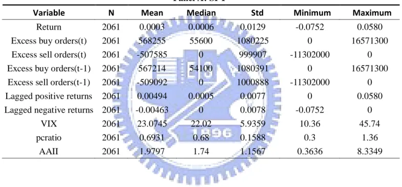
Panel A of Table 1 reports the descriptive statistics for SPY, and Panel B for QQQQ. The descriptive statistics include mean, median, standard deviation, maximum, and minimum. The average returns in SPY model is 0.03%, and in QQQQ model is -0.08%. The standard deviation of returns in SPY model is smaller than that in QQQQ model, and this is because the characteristics of the component stocks in QQQQ are similar to small stocks. The means of VIX, put-call ratio, and AAII in SPY model are 23.0745, 0.6931, and 1.9797, respectively. The means of VXN, put-call ratio, and AAII in QQQQ model are 43.6440, 0.7740, and 1.8613, respectively.
Panel C presents the correlation coefficients for SPY, and Panel D for QQQQ. As we can see in these two panels, the correlation coefficients among the investor sentiment indicators are significant in both SPY and QQQQ model. Except for AAII, the dependent variable almost correlated significantly the independent variables. The lagged positive and negative returns significantly correlate investor sentiment indicators. The correlation coefficients between investor sentiment indicators and order imbalances seem to be less significant, especially in QQQQ model.
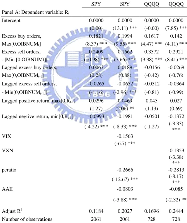
Table 2 shows the empirical results of the Equation 1 which consists of two targeted ETFs and the models with or without sentiment indicators. All the figures in Table 2 have been standardized, but the raw data are used in Table 1. The contemporaneous order imbalances are significantly and positively related to ETF returns in all ETF models. This relationship implies that excess buy (sell) orders drive up (down) market returns. This result is consistent with the empirical consequence of Chordia et al. (2002). However, according to Chordia et al. (2002), it seems unlikely that order imbalances can be a sign of a profit opportunity because only specialists know order imbalances in real time for individual stocks and no specialists know
3
order imbalances for all stocks in aggregate. Furthermore, the one-day lagged order imbalances seem to have no significant influence on ETF returns in our empirical results, and only the lagged excess sell orders are significant in the SPY model with sentiment. The lagged negative returns are significantly and negatively related to the ETF returns. The lagged positive returns are significantly related to the ETF returns in the SPY model with sentiment factor; however, under other conditions, the relationship is insignificant. This implies that only the past negative returns are related to contemporaneous returns, and the predictive power of the past positive returns is unclear.
As can be seen in table 2, the relationship between investor sentiment indicators and ETF returns are negative. This result means when sentiment is high, the ETF returns are relatively low, and vice versa. According to the previous research and theories, both of the influencing directions between sentiment and market returns are supported. The empirical results indicate that the relationship is negative. On one hand, the viewpoint which Brown and Cliff (2004) propose in their paper may be right, namely the ‗bargain shopper‘ effect really exists. On the other hand, the ‗hold-more‘ effect is smaller than the effect of the ‗overreaction of noise traders‘ in the see-saw battle which is mentioned in the papers of De Long et al. (1990) and Lee et al. (2002). As a result, the negative relationship between ETF returns and investor sentiment indicators is consistent with the previous theories.
Moreover, VIX and VXN are the indicators standing for implied volatility of S&P 500 and Nasdaq 100, respectively. The put-call ratio equals total trading volume of put option contracts divided by total trading volume of call option contracts. In this paper, we measure AAII by the ratio of the bearish percentage to the bullish percentage. Although all of these indicators may represent different meanings originally, they can be a symbol of investor sentiment in different aspects to explain
investor sentiments.
The next part of Table 2 demonstrates the adjusted R2 for the models with or without investor sentiment indicators. It is obvious that the adjusted R2 of the models with or without sentiment indicators increase largely. This result means that the three new-coming investor sentiment indicators certainly have explanatory power on market returns, and this is consistent with previous research.
To sum up, we find that investor sentiment indicators really have the marginal explanatory power on market returns beyond the contemporaneous order imbalances and lagged negative returns. This discovery also reveals that investor sentiment indicators can be used as a sign of predicting investment opportunity, and it proves that our first hypothesis is significantly valid. There is something vague, however, about the influencing directions of investor sentiment indicators on market returns. Although some scholars believe that the relationship between investor sentiment and market returns is positive from their empirical studies, there are other theories stating that the changing direction is negative. We think this difference may result from the chosen variables. The confusion about the changing directions and the using timing of sentiment indicators still need more detailed studies in the future to resolve.
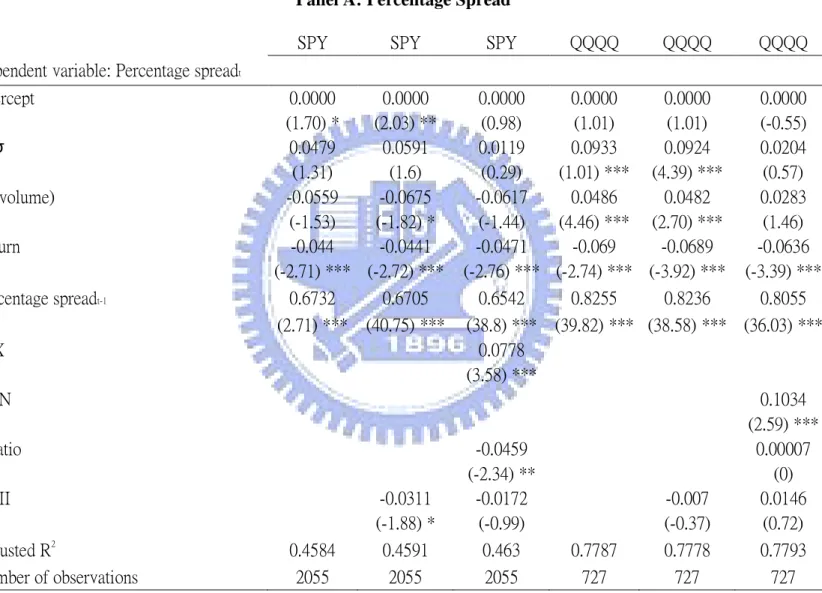
4.2 Liquidity Model with Sentiment
To examine the effect of investor sentiment indicators on market liquidity, we construct a liquidity model with investor sentiment, such as Equation 2 and 3.4 The second hypothesis of this paper hopes to find the relationship between market
liquidity and investor sentiment indicators to provide the references for the authorities and market makers. All the figures in Table 5 have been standardized, but the raw
4
We drop the lagged investor sentiment indicators because VIX series indicators have strong collinearity.
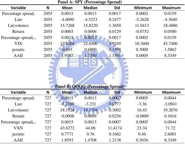
data are used in Table 3 and 4.
As can be seen in Table 3, it shows the descriptive statistics of the four models. The difference of the number of observations is because of the data quantity. The means of the percentage spread models are both 0.0015, while the standard deviations are 0.0017 and 0.0007, respectively. The means of the two OIBNUM models are 60672.4248 and -504960, while the standard deviations are 56860.73 and 3221625, respectively.
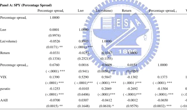
Table 4 provides the Pearson correlation coefficients of the variables of Equations 2 and 3. It shows that the correlations between market liquidity variables and investor sentiment indicators are generally significant, but the directions are not certain. This result suggests that the correlation between investor sentiment indicators and market liquidity variables is still unclear. There is a negative correlation between returns and percentage spread, but a positive correlation between returns and OIBNUM. This correlation implies that when returns increase, percentage spread decreases and thus market liquidity is high. On the other hand, when returns increase, OIBNUM increases and thus net buying pressure is high. Moreover, the correlation between market liquidity variables and one-term lagged market liquidity variables are positive.
Table 5 presents the empirical results of Equation 2 and 3. Panel A is for percentage spread models, and Panel B is for OIBNUM models. Each panel is separated into three parts: without sentiment indicators, only with AAII, and with three sentiment indicators (full model). It can be seen in Panel A that returns, one-term lagged percentage spread, VIX and VXN are significantly related to the contemporaneous percentage spread. From the third column, we can see that AAII in the SPY model is significant. The other two investor sentiment indicators in the full model, put-call ratio and AAII, are found to have no significant relationship with the
contemporaneous percentage spread except for put-call ratio in SPY models. The adjusted R2 for these two models are amazingly high at 46.3% and 77.93%, respectively. Nonetheless, when comparing the models with investor sentiment indicators and the models without investor sentiment indicators, the adjusted R2 do not apparently increase. The adjusted R2 decreases in the QQQQ model only with AAII. The significant variables in the models without sentiment indicators are also significant in the models with sentiment indicators. From Panel B, it can be seen that only returns for both of the SPY and QQQQ models and one-term lagged OIBNUM in the SPY model are significantly related to the contemporaneous OIBNUM. All of the investor sentiment indicators are insignificantly related to the contemporaneous OIBNUM. The adjusted R2 of the two OIBNUM models are dramatically lower than those of the two percentage spread models. The figures are 11.48% and 16.26%, respectively. Again, comparing the models with investor sentiment indicators and the models without investor sentiment indicators, the adjusted R2 just increases only marginally. It is worth paying attention that the adjusted R2 decreases in the QQQQ model only with AAII. The significant variables in the models without sentiment indicators are also significant in the models with sentiment indicators.
Baker and Stein (2004) propose a model to demonstrate that market liquidity can be an investor sentiment indicator under the condition with short-sale constraint. The model features a class of irrational investors who underreact to the information contained in order flow, thereby increasing market liquidity. In the presence of short-sales constraints, high liquidity is a symptom of the fact that the market is dominated by these irrational investors, and hence is overvalued. Thus, high liquidity is a sign that the sentiment of the irrational investors is positive.
The empirical results reveal that investor sentiment seems to be unrelated to market liquidity. As Baker and Stein (2004) mentioned, market liquidity is another
aspect of investor sentiment. That means that market liquidity is just one of the investor sentiment factors. Therefore, it is not appropriate to explain market liquidity by investor sentiment indicators, even by the market-based investor sentiment indicators which can reflect investors‘ perspectives of the future of the contemporaneous capital market.
On the other hand, some investor sentiment indicators are lagging indicators, such as AAII, the survey-based investor sentiment indicator. AAII is produced by surveying investors‘ viewpoints about the future capital market. The information contained in AAII has been thoroughly reflected in the capital market. From the empirical results, we can see that adding AAII into our model will decrease the adjusted R2. The results reveal that AAII is not an appropriate predicting indicator for market liquidity. Consequently, that is why AAII cannot explain the variation of liquidity variables. From the empirical results, AAII is insignificantly related to the dependent variables, percentage spread and OIBNUM. This result also proves the previous inferences.
Furthermore, percentage spread is related to price, and OIBNUM is related to trading volume. The empirical results reveal that the price-related market liquidity variable known as percentage spread can be explained more easily by our liquidity model. The R2 of the volume-related market liquidity variable OIBNUM is much smaller than that of the price-related market liquidity variable, percentage spread.
Nevertheless, the insignificant empirical results may come from the incorrect choice of variables. In Equations 2 and 3, almost only returns are significant in every model, and the one-term lagged percentage spread is significant in percentage spread models. From previous research, it has been proved that these two independent variables are significantly related to market liquidity variables. It is also possible that market liquidity is unrelated to investor sentiment indicators. This problem requires
further empirical tests in the future to resolve.
5. Conclusions
In this paper, the attempt is to find whether investor sentiment indicators can be used to explain market returns and market liquidity. The former has been tested by many other studies. The latter is a new issue which has seldom been mentioned in previous research. The market-based and survey-based investor sentiment indicators are simultaneously used in this study. The study hopes to discover the practical usefulness of investor sentiment indicators not only for forecasting the fluctuation of the market but also for providing a reference to the authorities, market makers and the related practitioners.
In our study, we amend the liquidity model of Chordia et al ―(2002) by adding investor sentiment indicators. The first hypothesis posits that the amended model can increase the explanatory power. Although the empirical result proves this hypothesis, the relationship between investor sentiment indicators and market returns seems to have room for further discussion.
In the second hypothesis, some factors are chosen to catch the variation of the market liquidity variables, particularly investor sentiment indicators. The second hypothesis postulates that market liquidity variables, percentage spread and OIBNUM, can be explained by investor sentiment indicators. The empirical result shows that investor sentiment indicators have little explanatory power in market liquidity variables despite the fact that the other independent variables in equation 2 and 3 seem to have better explanatory power on the market liquidity variables, especially on the percentage spread. These unanswered questions in the second hypothesis still need more thorough research in the future.
Overall, the research covering investor sentiment is relative new. There are unknown dimensions which are waiting to be discovered. This paper provides evidence to prove that investor sentiment can be used to predict market returns but maybe not be useful for predicting market liquidity. So far, the research into the relationship between investor sentiment and market liquidity is still incomplete. The field of investor sentiment requires more research to thoroughly explore the possibility.
References
Amihud, Yakov, 2002, Illiquidity and stock returns: cross-section and time-series effects, Journal of Financial Markets, 5, 31–56
Amihud, Yakov, and Haim Mendelson, 1986, Asset pricing and the bid–ask spread,
Journal of Financial Economics, 17, 223–249
Baker, Malcolm and Jeremy C. Stein, 2004, Market liquidity as a sentiment indicator,
Journal of Financial Markets 7, 271-299
Baker, Malcolm, and Jeffrey Wurgler, 2006, Investor sentiment and the cross-section of stock returns, Journal of Finance, 61, 1645-1680
Baker, Malcolm, and Jeffrey Wurgler, 2007, Investor sentiment in the stock market,
Journal of Economic perspectives 21, 129–151
Benston, George J., Robert L. Hagerman, 1974, Determinants of bid–asked spreads in the over-the-counter market, Journal of Financial Economics 1, 353–364 Blume, Marshall E., A. Craig MacKinlay, and Bruce Terker , 1989, Order imbalances
and stock price movements on October 19 and 20, 1987, Journal of Finance, 44, 827–848.
Brennan, M., and Avanidhar Subrahmanyam, 1996, Market microstructure and asset pricing: on the compensation for illiquidity in stock returns, Journal of
Financial Economics, 41, 441–464
Brown, Gregory and Michael Cliff, 1999, Sentiment and the stock market, Manuscript in preparation, University of North Carolina at Chapel Hill
Brown, Gregory W. and Michael T. Cliff, 2004, Investor sentiment and the near-term stock market, Journal of Empirical Finance 11, 1 –27
Brown, Philip, David Walsh, and Andrea Yuen, 1997, The interaction between order imbalance and stock price, Pacific-Basin Finance Journal 5, 539–557
Chan, Kalok, and Wai-Ming Fong, 2000, Trade size, order imbalance, and the volatility–volume relation, Journal of Financial Economics 57, 247–273
Chordia, Tarun, Richard Roll, and Avanidhar Subrahmanyam, 2000, Commonality in liquidity, Journal of Financial Economics 56, 3–28
Chordia, Tarun, Richard Roll, and Avanidhar Subrahmanyam, 2001, Market liquidity and trading activity, Journal of Finance 56, 501-530
Chordia, Tarun, Richard Roll, and Avanidhar Subrahmanyam, 2002, Order imbalance, liquidity, and market returns, Journal of Financial Economics 65, 111–130 Chung, Huimin, 2006, Investor protection and the liquidity of cross-listed securities:
Evidence from the ADR market, Journal of Banking & Finance 30, 1485–1505
Clarke, R. and M. Statman, 1998, Bullish or bearish? Financial Analysts Journal 4, 63–72
Datar, Vinay T., Narayan Y. Naik, and Robert Radcliffe, 1998, Liquidity and stock returns: an alternative test, Journal of Financial Markets 1, 203-219
D‘Avolio, Gene, 2002, The market for borrowing stock, Journal of Financial
Economics 66, 271-306
De Long, J. Bradford, Andrei Shleifer, Lawrence H. Summers, and Robert J. Waldmann, 1990, Noise trader risk in financial markets, Journal of Political
Economy 98, 703-738
Domowitz, Ian, Jack Glen, and Ananth Madhavan, 2001, Liquidity, volatility and equity trading costs across countries and over time, International Finance 4, 221-255
Fung, Joseph K.W., 2007, Order imbalance and the pricing of index futures, Journal
Fung, Joseph K.W. and Philip L.H. Yu, 2007, Order imbalance and the dynamics of index and futures prices, Journal of Futures Markets 27, 1129–1157
Fisher, Kenneth L. and Meir Statman, 1999, The sentiment of investors, large and small, working paper, Santa Clara University
Glushcov, Denys, 2005, Sentiment betas, working paper, University of Texas
Hasbrouck, Joel, Duane J. Seppi, 2001, Common factors in prices, order flows and liquidity, Journal of Financial Economics 59, 383–411
Huang, Roger D., and Hans R. Stoll, 1996, Dealer versus auction markets: A paired comparison of execution costs on NASDAQ and the NYSE, Journal of
Financial Economics 41, 313–357.
Jones, Charles and Owen Lamont, 2002, Short Sale Constraints and Stock Returns,
Journal of Financial Economics 66, 207-39
Kraus, Alan and Hans R. Stoll, 1972a, Parallel trading by institutional investors,
Journal of Financial and Quantitative Analysis 7, 2107–2138
Kraus, Alan and Hans R. Stoll, 1972b, Price impacts of block trading on the New York Stock Exchange, Journal of Finance 27, 569–588
Lauterbach, Beni, and Uri Ben-Zion, 1993, Stock market crashes and the performance of circuit breakers: empirical evidence, Journal of Finance 48, 1909–1925 Lee, Charles M.C., and Mark J. Ready, 1991, Inferring trade direction from intraday
data, Journal of Finance 46, 733-747
Lee, Wayne Y., Christine X. Jiang, and Daniel C. Intro, 2002, Stock market volatility, excess returns, and the role of investor sentiment, Journal of Banking and
Finance 26, 2277-2299
Rattray, Sandy and Devesh Shah, VIX Whitepaper, CBOE, 2003
Simon, David P., and Roy A. Wiggins III, 2001, S&P futures returns and contrary sentiment indicators, Journal of Futures Markets 21, 447–462
Shleifer, Andrei, and Robert Vishny, 1997, The limits of arbitrage, Journal of Finance 52, 35-55
Stoll, Hans R., 1978a, The supply if dealer services in securities markets, Journal of
Finance 33, 1133-1151
Stoll, Hans R., 1978b, The pricing of security dealer services: an empirical study of NASDAQ stocks, Journal of Finance 33, 1153–1172
Wang, Yaw-Huei, Aneel Keswani, and Stephen J. Taylor, 2006, The relationships between sentiment, returns and volatility, International Journal of
Appendix: Data process flow
1. Deleting the unnecessary and wrong data:
a. If the quote prices and quote volumes retrieved in the same second is identical to another set, then one set is deleted.
b. If the bid or ask price is equal to or less than zero, the datum is deleted. c. If the bid or ask volume is equal to or less than zero, the datum is deleted. d. If the traded price or volume is equal to or less than zero, the datum is deleted. e. The quote datum with bid-ask spread <0 or bid-ask spread>4 is deleted. f. Pt is trade price. If
Pt Pt1
/Pt1 0.1, the datum is deleted.Note: The t and t-1 refer two adjacent trades because the trades are viewed as continuous trades. The following g and h are the same. We only compare these three criteria in the trading time (9:30:00~16:01:00).
g. at is ask price. If
t
t1
/
t1 0.1, the datum is deleted. h. bt is bid price. If
bt bt1
/bt1 0.1, the datum is deleted.i. All trades and quotes which are beyond the trading time are deleted. Here we adopt 9:30:00~16:01:00 as our trading time. We choose 16:01:00 because there are still many large trades occurring after 16:00:00, and we need to cover those trades. j. If there are quoting data in one day but no trading data in the same day, the
additional quoted datum is deleted. 2. Merging data:
a. If there are many trading data in the same second, only the first one is reserved. b. According to the trading data, we merge the quoting data by matching the time of
the quoting data before one second or the older time of the trading data.
which is the largest sum of the bid quantity and ask quantity, is chosen. If that still cannot choose the single quote, the one with the smallest bid-ask spread is selected.
d. If there are no one-second-old quoting data, the first trading datum with the last-one-second or older quoting datum of the trading day before this trading day is merged.
e. Attention. For alleviating the work of the next section of distinguishing the orders, we need to reserve the five-second-old or older quoting data (comparing the time of the trading data). As a result, some quoting data before the time of the trading (before 9:30:00) should be reserved.
f. We only reserve the quoting data which is the largest quantity in every point of time.
3. Distinguishing the buyer-initiated or seller-initiated orders:
In this section, we compare the traded price with the midpoint of the ask and bid prices at least five seconds earlier. It is possible that the two traded price match the same midpoint of the ask and bid prices occurring at least five-second-old.
a. If the traded price is higher than the middle of the quote price occurring at least five seconds earlier, this trade is classified as being buyer-initiated.
b. If the traded price is lower than the middle of quote price occurring at least five seconds earlier, this trade is classified as being seller-initiated.
c. If the traded price is equal to the middle of quote price occurring at least five seconds earlier, we do the tick test. This is used to compare the traded price at time t with the traded price at time t-1.
Tick test 1: Here Pt and Pt-1 are compared. Pt is the current traded price. Pt-1 is the
previous traded price.
If Pt is lower than Pt-1, the trade is classified as seller-initiated.
If Pt is equal to Pt-1, the tick test 2 is done.
Tick Test 2: Here Pt and Pt-2 are compared. Pt-2 is traded price before the previous
traded price.
If Pt is higher than Pt-2, this trade is classified as being buyer-initiated.
If Pt is lower than Pt-2, this trade is classified as being seller-initiated.
If Pt is equal to Pt-2, this trade is deleted.
4. Printing out liquidity variables (daily data):
a. Percentage spread: After deleting the unnecessary and wrong trades and quote from the data, the percentage spread is calculated. The formula is ask price − bid price ask price + bid price /2 . Every percentage spread is summarized in every second and then the average is calculated to be a daily data.
b.OIBNUMt (Net buying pressure): The buyer-initiated orders are assigned +1, and
the seller-initiated orders are assigned -1. Then the trade volumes are multiplied and they are summarized on a daily basis. This is the second liquidity variable.
Table 1 Summary Statistics for Equation 1
This table provides the descriptive statistics and correlation coefficients for the variables in equation 1. The variables include returns, contemporaneous and lagged excess buy and sell orders, lagged positive and negative returns, and investor sentiment indicators. The data range covers from 1995 to 2003 for SPY, and from 2001 to 2003 for QQQQ. Panel A reports the description statistics for SPY, and Panel B for QQQQ. Panel C reports the correlation coefficients for SPY, and Panel D for QQQQ. In Panel C and D, p-values are in parentheses. *, **, and *** indicate that the coefficient estimates are statistically significant at the 0.1 level, 0.05 level, and 0.01 levels, respectively.
Panel A: SPY
Variable N Mean Median Std Minimum Maximum Return 2061 0.0003 0.0006 0.0129 -0.0752 0.0580 Excess buy orders(t) 2061 568255 55600 1080225 0 16571300 Excess sell orders(t) 2061 -507585 0 999907 -11302000 0 Excess buy orders(t-1) 2061 567214 54100 1080391 0 16571300 Excess sell orders(t-1) 2061 -509092 0 1000888 -11302000 0 Lagged positive returns 2061 0.00494 0.0005 0.0077 0 0.0580 Lagged negative returns 2061 -0.00463 0 0.0078 -0.0752 0
VIX 2061 23.0745 22.02 5.9359 10.36 45.74 pcratio 2061 0.6931 0.68 0.1588 0.3 1.36
Panel B: QQQQ
Variable N Mean Median Std Minimum Maximum Return 728 -0.0008 0.0007 0.0255 -0.0889 0.1016 Excess buy orders(t) 728 911882.47 0 1982138 0 21868500 Excess sell orders(t) 728 -1420806.35 -476200 1962749 -13450900 0 Excess buy orders(t-1) 728 909128.77 0 1982556 0 21868500 Excess sell orders(t-1) 728 -1431541.65 -480900 1972096 -13450900 0 Lagged positive returns 728 0.0094 0.0009 0.0149 0 0.1016 Lagged negative returns 728 -0.0102 0 0.0155 -0.0889 0
VXN 728 43.6440 44.07 11.4186 23.34 71.72 pcratio 728 0.7740 0.76 0.1521 0.46 1.36
Panel C: SPY Return Excess buy orders(t)
Excess sell orders(t)
Lagged excess buy orders(t-1) Lagged excess sell orders(t-1) Lagged positive returns Lagged negative
returns VIX pcratio AAII Return 1.0000 Excess buy orders(t) 0.2539 1.0000 (<0.0001)*** Excess sell orders(t) 0.2751 0.2672 1.0000 (<0.0001)*** (<0.0001)***
Lagged excess buy
orders(t-1) 0.0103 0.0665 0.0098 1.0000 (0.6419) (0.0025)*** (0.6573)
Lagged excess sell
orders(t-1) -0.0269 -0.0680 0.1575 0.2672 1.0000 (0.2227) (0.002)*** (<0.0001) (<0.0001)*** Lagged positive returns 0.0081 0.0475 0.0387 0.3000 0.1378 1.0000 (0.7136) (0.0311)** (0.079) (<0.0001)*** (<0.0001)*** Lagged negative eturns -0.0749 -0.0384 0.1156 0.1240 0.3190 0.3795 1.0000 (0.0007)*** (0.081)* (<0.0001)*** (<0.0001)*** (<0.0001)*** (<0.0001)*** VIX -0.1297 0.0951 -0.2520 0.0945 -0.2415 0.1045 -0.3090 1.0000 (<0.0001)*** (<0.0001)*** (<0.0001)*** (<0.0001)*** (<0.0001)*** (<0.0001)*** (<0.0001)*** pcratio -0.2712 -0.0324 -0.1982 -0.0700 -0.1654 -0.1244 -0.2554 0.2099 1.0000 (<0.0001)*** (-0.141) (<0.0001)*** (0.0015)*** (<0.0001)*** (<0.0001)*** (<0.0001)*** (<0.0001)*** AAII -0.0015 -0.0101 0.0677*** -0.0006 0.0552** -0.0870*** 0.0502** -0.2722*** -0.1679*** 1.0000 (0.9475) (-0.6463) (0.0021) (0.7722) (0.0122) (<0.0001) (0.0227) (<0.0001) (<0.0001)