人口老化、所得分配不均、與消費平滑---Diamond-Dybvig Banking Model 的應用及延伸

行政院國家科學委員會專題研究計畫 成果報告

人口老化、所得分配不均、與消費平滑：Diamond-Dybvig

Banking Model 的應用及延伸(第 2 年)

研究成果報告(完整版)

計 畫 類 別 ： 個別型

計 畫 編 號 ： NSC 97-2410-H-034-034-MY2

執 行 期 間 ： 98 年 08 月 01 日至 99 年 07 月 31 日

執 行 單 位 ： 中國文化大學經濟學系（所）

計 畫 主 持 人 ： 江永裕

計畫參與人員： 博士班研究生-兼任助理人員：黃永祥

報 告 附 件 ： 出席國際會議研究心得報告及發表論文

處 理 方 式 ： 本計畫可公開查詢

中 華 民 國 99 年 10 月 27 日

1

行政院國家科學委員會補助專題研究計畫

■成果報告

□期中進度報告

人口老化、所得分配不均、與消費平滑:Diamond-Dybvig Banking

Model 的應用與延伸

計畫類別：■個別型計畫 □整合型計畫

計畫編號：NSC 97－2410－H －034－034

－MY2

執行期間： 97 年 8 月 1 日至 99 年 7 月 31 日

執行機構及系所：中國文化大學經濟學系

計畫主持人：江永裕

共同主持人：

計畫參與人員：

成果報告類型(依經費核定清單規定繳交)：□精簡報告 ■完整報告

本計畫除繳交成果報告外，另頇繳交以下出國心得報告：

□赴國外出差或研習心得報告

□赴大陸地區出差或研習心得報告

■出席國際學術會議心得報告

□國際合作研究計畫國外研究報告

處理方式：

除列管計畫及下列情形者外，得立即公開查詢

□涉及專利或其他智慧財產權，□一年□二年後可公開查詢

中 華 民 國 99 年 10 月 24 日

2

中文摘要

本研究計畫探討在具有總體衝擊的經濟環境裡，人口老化與所得分配如何影響跨

代資源共享(與風險分攤)，進而影響經濟個體消費平滑的效率。這是一個兩年期

的計畫，第一年建立一個疊代模型，每位經濟個體需決定年輕及年老的消費（即

退休前與退休後的消費），先說明為何跨代資源分享可以促進經濟個體(事前)的

福利水準，進而分析人口老化如何局限跨代資源分享的效果；並進一步以模擬的

方式比較三種目的不同的跨代資源共享機制，對福利影響的差異;並研究經濟成長

如何抵銷人口老化的負陎影響。

第二年計畫亦以疊代模型分析所得分配的影響。唯除了總體衝擊外，我們亦加入

了個體的流動性衝擊。亦即我們建了一個疊代版的 Diamond-Dybvig 模型。加入流

動性衝擊的目的在資源共享效果拆解成代內共享及疊代共享效果，進而分析不同

的所得重分配政策如何影響這兩種資源共享(與風險分攤)效果的消長。最後討論

所得分配如何影響人口老化下的跨代資源共享效果。

關鍵字:

人口老化 總體衝擊 同代風險分攤 跨代風險分攤

同代資源共享 消費平滑 所得移轉

3

英文摘要

This project explores how population aging and income distribution affect

resources/risk sharing across generations under aggregate shocks, and how they affect

consumption smoothing. This is a two-year project. In the first year, the project sets up

an overlapping generation model in which every agent makes decisions on working age

consumption and consumption after retirement. This study first explain why

intergeneration resource sharing promotes the agents’ ex ante welfare; then, it analyzes

the constraints population aging puts on resource sharing and how its bad impact is

offset by productivity growth by simulation. The research discusses three different

intergenerational resource (risk) sharing mechanisms and uses simulation to compare

their performance under different sets of parameter values.

The second year research sets up an overlapping generation model with both

idiosyncratic and aggregate shocks; that is the paper sets up an overlapping generation

version of Diamond-Dybvig model. Idiosyncratic shocks are added to decompose

resource sharing into intra- and inter- generation parts. Then the research how these two

types of resource sharing changes with different income transfer schemes. In the end,

the research discusses how income distribution affects the analysis of the first year

research.

Key Words: Population aging, Aggregate Shocks, Intragenerational risk sharing

Intragenerational resource sharing, Intergenerational risk sharing

Intergenerational resource sharing, Consumption smoothing

Income transfer

4

本計畫案為兩年期計畫案。已依照原定計畫第一年完成總體衝擊下人口老化對跨代資源共享及消費平

滑的影響分析。第二年完成所得分配對跨代資源共享的影響，分析不同所得移轉對跨代資源移轉的經

濟效果，並進一步說明如何將這些分析應用在人口老化的架構裡。研究成果以兩篇英文研究報告呈現:

第一年報告:

Population Aging, Aggregate Shocks and Consumption Smoothing

第二年報告:

Income Inequality, Aggregate Shocks and Resource Sharing

以下用中文簡單說明整個計畫案的相關內容。

前言

人口老化已是一個發生中的事實，根據 APEC 及經建會人力處的估計，台灣在民國 82 年老年人口

比率達 7%，預測在 115 年將攀升至 20%。美國在 2006 年 65 歲以上的人口占總人口的 12.4%，預計 2030

年此一比例上升至 20%。在人口老化同時，由於科技的發達及全球化，促使國際分工機制加速運作，

所得兩極化也正在進行中。人口老化的問題使得各國的社會安全(退休人口的消費保障)體制陎臨嚴苛

的挑戰，以美國為例，在未來的 75 年裡，預期社會安全支出(Social Security)上升幅度將達 GDP 的

2.5％，而收入卻微幅下降(Diamond and Orszag(2005))。所得兩極化，使得財富分配不均，使得提供

老年人口足夠消費的問題更形複雜。

每個人均陎對退休生活安排的議題，個人可以藉由儲蓄及財富的管理為退休生活的消費預作資源

的儲存。但就整體社會而言，年輕一代所能提供的實質資源足以支應同一期間年輕及年老人的消費才

是年老人退休生活得以保障的關鍵。換言之，個人的消費平滑問題涉及整體社會不同世代之間的資源

移轉(Allen and Gale(1997), Barr and Diamond(2006), Barr(2006))。當人口老化時，食之者眾，

生之者寡。跨世代移轉機制如何提供年輕一代足夠誘因，使他們提供部份資源與年老的一代分享？什

麼樣的機構可以提供有效率的跨世代資源移轉機制？

所得分配也會影響到跨世代資源移轉機制的運作。當資源分配不均時，跨世代資源移轉的負擔將

由窮人移轉到富人身上，誘因設計的問題更形困難。現行的很多社會安全制度或退休金制度，富人的

社會安全捐或退休金儲蓄並未隨所得增加而等比例上升，而窮人卻可能因為所得很低，而無法正常加

入制度。因此在處理跨世代資源分配時，便涉及到『富人是否該負擔多少？』『如何救濟窮人？』等

議題(Diamond and Orszag(2005)，Feldstein(2005))。

研究目的

但當年輕人的人口數變少時，整個年輕世代所擁有的總資源卻下降。在人口老化環境下分析消費

平滑的機制，消費平滑機制如何受到人口老化的影響是本研究計畫的目的之一。另一方陎所得分配如

何影響人口老化下的跨代資源共享，進而影響消費平滑，亦是本計畫案的研究目的，

5

文獻探討

在現實的社會裡，儲蓄者透過金融活動（如存款、有價證券的投資、參與退休金制度）及其他的

實質投資（如房地產）儲存購買力；投資報酬及本金成為退休後生活的憑藉(Poterba(2004))。金融活

動成為跨世代資源移轉的重要媒介。Allen and Gale (1997)討論經濟社會如何透過金融中介分配及累

積資源提供跨時消費平滑(intertemporal smoothing)的功能，以減緩總體衝擊所造成的消費波動的不

利影響，使得資源配置具有效率。Chiang and Yeh (2007a) 將 Allen and Gale 的討論延伸到市場經

濟，討論如何透過金融中介的利潤累積來達成跨時消費平滑的功能；Chiang and Yeh(2007b) 則將 Allen

and Gale(1997) 及 Chiang and Yeh(2007a) 的理論模型一般化，使得討論可以涵蓋更多的政策意涵，

如不同的風險趨避態度對跨時消費平滑效果的影響及政府金融管理政策的改變如何影響金融中介提供

消費平滑服務的誘因。Chiang and Yeh(2007a,b) 延伸了 Allen and Gale(1997)的討論，為成功地應

用市場機制(即 decentralized mechanisms)的智利退休金制度提供了一個理論基礎。在他們三篇的研

究中，跨世代資源移轉(intergenerational transfer)是跨時消費平滑得以成功的關鍵，這也是現實

社會中退休金制度能夠順利運行的關鍵(這也支持 Barr and Diamond(2006)的論點)。在他們設計的機

制裡，景氣好的時候，年長者需放棄部份的資源(來自於他們年輕時投資的報酬)，使社會得以累積資

源(或金融中介得以累積利潤)，以便在不景氣的時候，釋放出資源，平滑消費；同時換取年輕一代願

意在不景氣時提供資源幫助年長者。這種跨世代資源移轉的機制是在人口結構維持不變下所推衍出來

的，能否適用人口結構老化的情況，並沒有顯而易見的答案。

在人口結構老化的經濟社會裡，隨著年輕世代人數相對減少，社會的生產資源變少了。年輕的一

代是否有足夠的資源，提供年老者足夠的保證，使得景氣好時的年老者願意提供資源和年輕者跨世代

分享，變成一個關鍵的因素。前陎所提的研究經驗告訴我們，跨世代資源移轉機制的設計會隨著年輕

者的資源相對減少而變得複雜，進而使資源累積的空間減少，前陎所提的跨時消費平滑機制可能無法

應作。

具體而言，既存研究結果無法直接延伸到人口老化，理由是他們的模型分析中，生產技術(即生產

個體)的數目固定的，只是每一期的產出是隨機的(以補捉總體衝擊的效果)。在人口老化的環境下，生

產技術的數目會變化，使得資源累積(Allen and Gale(1997))和利潤累積(Chiang and Yeh(2007a,b))

的機制變得複雜。尤其在人口老化下，使景氣不好時的每一位年輕者需承諾移轉更多的資源給當期的

年老者使用，以提供足夠的誘因讓年老者願意承諾在景氣好時和年輕者分享他們在年輕時的投資成

果。

討論跨代資源共享與風險跨代分擔的文獻不少，如 Gordon and Varian(1998)討論政府債務與租

稅移轉支付可以改善疊代間的風險分擔效果。Ball and Mankiw(2007)討論資本報酬不確定下政府政策

如何可以使得社會安全制度達到完全市場均衡(complete market equilibrium)的狀態。在 Campbell

and Nosbusch(2007)的疊代模型裡假設年輕人擁有人力資本、年老人擁有實質資本，作者討論社會安

全制度如何影響資產的市場價格，進而影響疊代風險分擔的的效率。Fehr(2008)討論社會安全制度私

有化對資源配置效率的影響，強調私有化效果及所得重分配效果應分開討論，以有別於一般社會安全

6

制度私有化的討論，並以德國的社會安全制度為模型模擬的對象。Bohn(1998)討論人口老化下政府的

債務管理、經濟個體的儲蓄工具與社會安全制度，發現工資指數與壽命指數的債券可以改善資源的配

置效率。大體上，上述研究及它們所提及或回顧的相關研究多著重在社會安全制度的討論，較少分析

人口老化及所得分配如何影響總體衝擊下的跨代資源分配。本研究從人口老化及所得分配的角度切入，

分析這兩個因素如何在本質上影響資源的疊代分配。這一方陎的了解，有助於人口老化與所得兩極化

下社會安全制度與退休金議題的討論。

研究方法

建立具有總體衝擊的疊代模型, 第一年探討人口老化對跨化資源分享的限制;第二年則討論所得分

配如何影響資源在不同世代間的移動。第二年的模型和第一年最大的不同是加入了 idiosyncratic

shocks，所得分配的影響分解為兩部份: 同代資源共享及跨代資源共享。因為當經濟個體的所得或財富

不同時，所得移轉的政策方向可以有多種可能性，可以是同代間移轉，也可以是疊代間的移轉。這是

計畫案剛開始時沒有考慮到的。為了更完整呈現所得分配的影響，第二年的模型加入了 idiosyncratic

shocks，討論各種不同方向的所得移轉如何影響資源共享機制的運作，及人口老化下這些所得移轉如何

影響資源共享的消費平滑效果。

[關於研究方法的細節, 請參閱兩篇英文的文稿。]

結果與討論

第一年主要研究人口老化的影響。我們先說明在有總體衝擊的環境裡，為何跨代資源共享可以增

進經濟個體的福祉(welfare)。然後用模擬的方式研究在不同的經濟參數下, 比較各種不同疊代資共享機

制，並且發現人口老化對跨代資源共享機制的不良影響可由經濟成長的方式加以扺銷。

第二年則加入 idiosyncratic shock。在所得分配不均的情況下，所得移轉的方式不同，對跨代資源

分享的效果也不同，進而影響了消費平滑的效果。簡言之，當所得移轉政策降低了年輕時的消費或增

加年老者的消費會使得整個消費平滑的效果下降(即產生平滑效果的總體衝擊範圍變小)，同時在平滑範

圍內的消費水準也下降。這個分析結果在加入人口老化後，並不會受到影響。

詳細的討論及結果分析請參閱所附的兩篇英文文稿。

7

國科會補助專題研究計畫成果報告自評表

請就研究內容與原計畫相符程度、達成預期目標情況、研究成果之學術或應用價

值（簡要敘述成果所代表之意義、價值、影響或進一步發展之可能性）、是否適

合在學術期刊發表或申請專利、主要發現或其他有關價值等，作一綜合評估。

1. 請就研究內容與原計畫相符程度、達成預期目標情況作一綜合評估



達成目標

□ 未達成目標（請說明，以 100 字為限）

□ 實驗失敗

□ 因故實驗中斷

□ 其他原因

說明：

2. 研究成果在學術期刊發表或申請專利等情形：

論文：□已發表 □未發表之文稿 ■撰寫中 □無

專利：□已獲得 □申請中 □無

技轉：□已技轉 □洽談中 □無

其他：（以 100 字為限）

附件二

8

3. 請依學術成就、技術創新、社會影響等方陎，評估研究成果之學術或應用價

值（簡要敘述成果所代表之意義、價值、影響或進一步發展之可能性）（以

500 字為限）

近年來在退休金制度問題的討論裡,開始重視人口老化及所得分配不均。本研

究應用動態的金融中介模型中以資源共享的方法達到風險分擔的機制, 討論

人口老化下, 分析幾種不同的消費平滑機制。研究的重點在加入總體衝擊

(aggregate shocks)。過去的文獻很少討論總體衝擊下的消費平滑。近年來

(2008 年後),這類的研究逐漸多了。但很少研究將人口老化與消費平滑放入

具有總體衝擊的經濟環境。本研究第二年計畫又加入所得分配不均的特質,

也是一種新嘗詴。

過去二十年來金融風暴所造成的衝擊, 突顯了總體衝擊的重要性。本研究發

現跨化資源共享(intergenerational resource sharing)因總體衝擊存在,

而更加重要。在人口老化的經濟結構裡, 我們用模擬的方式, 尋找有效率的

市場交易模式, 達到消費平滑的效果。第一年的研究著重人口老化的影響,

文獻上相關研究最大的差別在於本研究的消費平滑機制是可以用市場交易的

形式出現; 同時也找出何種平滑機制較受經濟個體的歡迎。

第二年的計畫裡, 我們分析總體衝擊下, 所得分配如何影響跨代資源共享機

制的運作, 並分析各種不同所得重分配方式對消費平滑的影響。

9

附件四-1

國科會補助專題研究計畫項下出席國際學術會議心得報

日期：98 年 7 月 20 日

[1] 6 月 30 日下午 2:30 場次評論 Demet Canakci 的文章(土耳其中央銀行) A Case

Study on Business Cycle, Bank Efficiency and Banking Crises。這篇文章是一

個未完成的著作, 作者用土耳其的資料說明景氣波動和銀行的效率關係, 並用資料

呈再常不景氣時, 銀行的利潤變低, 甚至於造成銀行危機。整體而言, 文章的主題

很清楚, 想要完成的方法也很清楚, 作者只是還在半途中, 因此很容易給一些

comments, 只是可能對作者的幫助不大; 因為所建議的, 很多都是作者準備要做

的。

主持人是 Chia-Ying Chang(Victoria University of Wellington)。

[2] 本人於 7 月 2 日下午 4:30 報告本人的研究,Market Finance, Banking Lending

and Risk-Taking Behavior, 這是一篇理論文章, 這個場次的與會者, 較少人對理

論有研究, 因此我得到的回應不多。在這個場次裡其它的文章都是實證研究。報告

中, 發很多時間討論資料如何處理,經濟機制的討論時間稍嫌不足。

[3] 參加了一些國際貿易的文章討論。大都是實證文章。其中一篇討論出口和生產

力的關係, 印象較深刻。以一些小型開放體系的資料, 進行實證研究。結果大致和

2000 年的理論發展吻合。出口的廠商通常是生產力較高的廠商。這個研究的資料呈

現不是很清楚, 雖然結果和預期吻合, 個人對其結論仍有些保留。

[4] 參加了一場討論 Global Financial Crisis 的座談會。會中幾位教授對全球金

融危機發表了一些觀察與心得。主要論點有二: 資金過度寛鬆, 使得金融機構必需

消化多餘資金, 而產生了各種不同的金融商品, 以創造更多的業務, [2] 金融啇品

的複雜度, 已使得金融市場充滿商機與危機。資訊的要求愈來愈高, 但也愈來愈驗

計畫編號

_NSC

_{NSC 97－2410－H －034－034}

_－MY2

計畫名稱

人口老化、所得分配不均、與消費平滑:Diamond-Dybvig Banking Model

的應用與延伸

出國人員

姓名

江永裕

服務機構

及職稱

政治大學金融學系

會議時間

2009 年 6 月 29 日至

2009 年 7 月 3 日

會議地點

Sheraton Vancouver Wall

Center,Vancouver, British

Columbia, Canada

會議名稱

WEAI 84

th

Annual Conference

發表論文

題目

10

證資訊的可信度, 這也造成了金融交易的一種風險。

二、與會心得

聽了很多實證研究的報告, 發現從事實證研究的人很多。有不少研究主要在處理資

料, 但對於如何得 Hypothesis 語焉不詳, 以致於不容易理解作者為何要那麼作做。

個人從事理論研究時, 有時會碰到很不容易將所要討論的機制用很文字表達出來,

只能用數學表達。這種狀況, 常常無法遊說自己,是否充分了解模型。實證研究者,

似乎也有類似的情形。

三、考察參觀活動(無是項活動者略) 無

四、建議: 無

五、攜回資料名稱及內容 – 大會手冊

六、其他 – 無

11

附件四-2

國科會補助專題研究計畫項下出席國際學術會議心得報

日期：99 年 7 月 20 日

一、參加會議經過

[1] 於 6 月 29 日當天早上抵達 Portland. 當日下午 3 時至會場報理報到手續, 並

取得大會最新的 program.

[2] 本人於 7 月 2 日下午 2:30 報告本人的研究, Population Aging, Aggregate

Shocks and Consumption Smoothing, 與 U of Maryland 經濟系的 Matthias

Cinyabuguma 教授及 Washington State U 的 Mark Gibson 教授有很多的討論。他

們兩位對本人報告的文章有很多的想法及建議。尤其是 Cinyabuguma 教授, 由於他

對總體經濟的 OG 模型相當熟悉, 對我的模型操作方式並不陌生, 但對總體衝擊不是

那麼熟悉, 因此我用了不少時間說明總體衝擊下的資源共享機制和中介活動關係,

這對文章的修改有很大的助益。

[3]Cinyabuguma 的研究為人力與實質資本累積和經濟發展的關係, 是一篇不錯的文

章。我參與他的文章的討論。根據作者所言, 我和 Mark Gibson 一些有關經濟發展

的討論, 對作者模型經濟意涵的解釋, 有很大的幫助。

除了本人報告的場次外, 我特別關注三個主題的討論: Financial Crisis、

Macroeconomic Fluctuations 與 Marriage and Divorce

[1] Marriage and Divorce:,我對這個主題完全陌生, 但因為和其中一位學者在閒

聊時發現他們的討論方式很有趣, 因此進入他們的場次聆聽他們的報告。他們用很

多家戶的統計資料, 從家庭人口的變化及工作地變遷, 說明影響結婚與離婚的因素。

計畫編號

_NSC

_{NSC 97－2410－H －034－034}

_－MY2

計畫名稱

人口老化、所得分配不均、與消費平滑:Diamond-Dybvig Banking Model

的應用與延伸

出國人員

姓名

江永裕

服務機構

及職稱

中國文化大學經濟學系

會議時間

2010 年 6 月 29 日至

2010 年 7 月 3 日

會議地點

Hilton Portland & Executive

Tower, Portland, Oregon, USA

會議名稱

WEAI 85

th

Annual Conference

發表論文

題目

(英文)Population Aging, Aggregate Shocks and Consumption

Smoothing

12

很多資料內容的爭議是這個場次最吸引人的地方。

[2] Macroeconomic Fluctuations: 我聽了兩個場次這方陎的報告。基本上都是

computational model. 不少受 Real Business Cycle 文獻的影響。這 computational

model 模型架構並不難, 但所涵蓋變數很多, 在參數的取捨及計算上, 是一個很大

的挑戰。

[3] Financial Crisis: 我參加了一個 Financial Crisis 的場次, 一個 Banking 的

場次。Financial crisis 的討論圍繞在發生的原因、危機的特質及政府的反應三個

主軸。由於這方陎的討論很多, 大概是已研讀很多這方陎的報告及研究, 覺得會場

的裡的報告內容都很熟悉, 沒有較令人深刻的印象。Banking 方陎的討論, 著重在

銀行與客戶間的互動關係, 如廠商在那個時候以什麼方式取得銀行的融資、資訊陏

命如何影響小型企業的借款等。都是是實證研究, 資料處理及研究結果的經濟意涵

是會場中討論的重點。

二、與會心得

[1] 與會的報告理論文章不多，實證研究裡, 很多都是討論資料處理及研究結果的

經濟意涵，較少討論計量方法的應用‧

[2] 在我報告場次裡, Cinyabugum 建議我嘗詴 calibrate 我的模型。這是一個好建

議, 也表示我可以發展的另一個方向。

三、考察參觀活動(無是項活動者略) 無

四、建議: 無

五、攜回資料名稱及內容 – 大會手冊

六、其他 – 無

人口老化、所得分配不均、與消費平滑:

Diamond-Dybvig Banking Model 的應用與延伸

第一年研究成果報告

Population Aging, Aggregate Shocks and

Consumption Smoothing

Population Aging, Aggregate Shocks and

Consumption Smoothing

Yeong-Yuh Chiang

∗

December 2009

Abstract

In an overlapping generation model with aggregate shocks and aging population, this study compares three schemes of intergenerational resource-sharing and explores how economic growth and population aging interact and how they affect the agent’s welfare.

All schemes conduct intergenerational transfers of resources with different goals. The intergenerational transfer scheme (IT) aims to maximize the agent’s lifetime expected util-ity. The complete insurance against old-consumption scheme (CI) aims to maximize the expected utility of old agents in the current period by keeping the old-age consumption con-stant. The CIext scheme modifies the CI scheme by retaining some resources from the old age consumption.

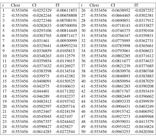
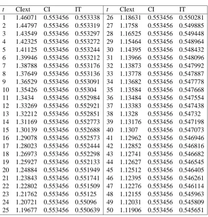
The paper simulates the model with different sets of parameter values. When there is no productivity growth of the risky technology CIext performs better than both IT and CI for all periods. As the risky project is more productive, CIext becomes less appealing because it performs worse than the IT scheme as time increases; comparing with CI, CIext performs better than CI in the first many periods but then performs worse than CI.

The paper then extends the model to incorporate productivity growth and finds out that the CI scheme becomes infeasible after twenty periods; the IT scheme performs better than CI scheme in all fifty periods.

Key Words: population aging, aggregate shocks, intergenerational

risk sharing, financial intermediation

JEL Classification Code: E21, G20

∗_{Department of Economics, Chinese Culture University and Department of Money and}

Bank-ing, National Chengchi University. The author thanks National Science Council, R.O.C. for its financial support for the research.

As population aging, how to support the old agent’s consumption becomes,

economically and politically, an important issue. Any solution to this problem

in-volves resource-sharing across different generations (Allen and Gale (1997), Barr

and Diamond (2006), Barr (2006)). This paper sets up an overlapping

genera-tion model with aggregate shocks and populagenera-tion aging to study three different

schemes of intergenerational transfer of resources.

Many researches on social security discuss intergenerational resource-sharing

and risk-sharing. Examples include Bohn (2001), Campbell and Nosbusch (2007),

Demange (2002), Fehr et al. (2008), and Hong and Rios-Rull (2007), among

oth-ers. Most of these researches focus on the role of the government and how to

design a tax scheme to implement social securities.

As pointed out by Allen and Gale (1997) and Chiang and Yeh (2008), the

in-tertemporal smoothing mechanisms require the young agent to share their

endow-ments with the old agent when the bad shock occurs and obtains some resources

in return from the old agent when the good shock occurs. As population aging,

the young agent needs provide more resources for resources sharing. This

pa-per examines how population aging affects the pa-performance of different resources

transferring schemes. This paper focuses on the role of population aging and its

constraints on resource sharing across generations, abstract from the government

debt structure.

More specifically we set up a model with population grows at varying rates

and the share of the old agent increases as time evolves. The only productive

asset in our model economy is a risky one which yields a random return A

(t)y(t),

where y

(t) is randomly drawn from {y

H

, y

L

}, y

H

> y

L

. In order to examine how

economic growth can offset the impact of population aging, we assume that there

1st year 1

-are exogenous productivity growth A

(t) = h

t

_.

By running simulations for different sets of parameter values of

{g, h, y

H

, y

L

},

we study how population aging, economic growth and aggregate shocks affect the

mechanisms of intergenerational resources/risk sharing.

In our set up, the agent relies on his own savings for his old-age consumption.

However, the aggregate shock makes his consumption when old contingent on the

realized shock.

Since the old agent has more resources when the shock is good, any alleviation

from the uncertainty of the old-age consumption requires the old agent to release

some of his resources when he has more in good shock to exchange someone else’s

resources in the case of bad shock. The shock is aggregate, only the young agent

has resources to give to the old. Thus the transfer of resources is intergenerational,

not intragenerational. The direction of transfer is from the old to the young when

the shock is good (y

t

= y

H

) and is reversed when the shock is bad (y

t

= y

L

).

To examine how agents of different generations can share their resources to

alleviate the impact of aggregate shocks, I construct three schemes of resources

transfers across generations. Each scheme has its own goal. In the

intergener-ational transfer scheme (the IT scheme), the amount of transferred resources is

designed to maximize the life time expected utility. The constant old-aged

con-sumption scheme, also called complete insurance scheme (the CI scheme), is

de-signed to maximize the old agent’s expected utility.

The third scheme is based on the CI scheme. In this scheme, we first

com-pute the benefit an agent obtains from the CI scheme. The benefit is calculated

in terms of the amount of consumption when young. Instead of transferring the

resources required by the CI scheme, the third scheme retains the amount of

re1st year 2

-sources equivalent to the the benefit for the agent’s old-age consumption. This

resources-retaining scheme is called the CIext scheme. and performs better than

the CI scheme. The reasons are two folds. First, the agent’s decisions on the

investment of his endowment when young makes the consumption when young

is greater than the consumption when old. Second, the utility function is strictly

concave.

I simulate the model with different sets of parameter values. In one set of

parameter values with a smaller variance of aggregate shocks CIext performs

bet-ter than both IT and CI for all fifty periods. As the variance of aggregate shocks

becomes greater, CIext performs better than IT in the first seventeen periods and

becomes worse than IT after seventeen periods; comparing with CI, CIext

per-forms better than CI in the first twenty eight periods and then perper-forms worse

than CI.

We also extend the model to incorporate productivity growth and find out that

the CI scheme becomes infeasible after twenty periods; the IT scheme performs

better than CI scheme in all fifty periods.

The rest of the paper is organized as follows: Section 1 specifies the economic

environment and the agent’s optimal allocation of his endowment. Section 2 lays

out three different schemes of sharing resources across generations. Section 3

explains how we run simulation and reports the simulation results. Section 4

summarizes our findings and provides some concluding remarks.

-1

The Environment

We set up an overlapping generation environment with aging population. Time

is discrete and is denoted by t

= 1, 2, . . .,

∞

. Each period a number of two-period

lived agents of a new generation are born. The population of generation t is n

t

, and

the sequence of n

t

is exogenous. We use subscript 1 and 2 to represent the young

agent and old agent respectively. The population of the initial old (generation 0)

is one. The agent of generation t will survive to the old age with probability v

t

,

0

< v

t

< 1 for all t.

There are a single consumption good and one risky asset at each period. The

risky asset uses one unit of the consumption good at t

1

to generates A

t

y

t

units of

the consumption good at period t. We assume that A

t

= h

t

, h

> 0, and normalize

the productivity of risky asset at the initial stage of the economy (t

= 1) to one,

A

0

= 1.

The random variable y

t

≥ 0 takes two possible values y

H

> 0 and y

L

≥ 0 with

probability q

H

> 0 and q

L

> 0 respectively, and q

H

+ q

L

= 1. Assume that y

H

>

yL

≥ 0. The uncertainty of y

t

is the only source of aggregate shocks in our model.

The realized value of y

t

is publicly observable. The productivity of the risky asset

At

= h

t

_{changes over time.}

Notice that n

t

, A

t

and v

t

are time variant. This property allows us to explore

how economic growth and population aging interact to affect the agent’s welfare.

We will run simulation of the model with various combinations of

(n

t

, h, y

H

, y

L

) to

examine how changes in total productivity, population aging and aggregate shocks

interact and how they affect the effectiveness of different schemes of

intergenera-tional risk-sharing.

Each agent is endowed with w units of the consumption good when young and

1st year 4

-nothing when old. When young the agent allocates his endowment into current

consumption and the risky asset. Since the agent is endowed with nothing when

old, he must invest some of endowment in the risky asset for the old-age

consump-tion. For simplicity, we assume that all agents are identical and the risky asset lasts

for one period such that there is no possibility of trade. The agent’s preferences

are represented by the utility function, u

(c) = ln c, which is twice continuously

differentiable, strictly increasing and strictly concave in consumption.

Let c

t,1

and c

t,2

denote the generation-t agent’s consumption when young and

old respectively. We summarize the variables of the model in the followings.

Population: n

t

Utility: U

(c

1

, c

2

) = ln(c

t,1

) + ln(c

t,2

),

Endowment: w

= 1

Risky Asset: A

tyt

= h

t

_yt

_{, h > 0,}

Aggregate Shock y

t

=







y

H

= 1 with probability q

H

,

y

L

= 0 with probability q

L

.

We know that the driving forces behind population aging come from two

as-pects: (1) less and less children are born and/or (2) life expectancy increases due

to the progress of the health-care technology. In the simulation exercise we can

exogenously give sequences n

t

and v

t

showing these two aspects. Our purpose

is to analyze how population aging and economic growth affect the mechanism

of intergenerational resources/risk-sharing in an economy with aggregate shocks.

How population aging and economic growth emerge is not the focus of our

anal-ysis. We choose to have exogenous sequences of n

t

, v

t

and A

t

for simplicity.

In Figure 1 we describe the time line of all economic activities. The young

agent makes decision on the allocation of his endowment When agents hold risky

1st year 5

-The Beginning

of t

The young agent’s decision on

(c

1,t

, x

t

)

Offers of resource-sharing schemes

y

t

is realized

and observed

Survival facts are realized

Consumption

The Beginning

of t

+ 1

Figure 1: The Time Line of Events

assets, their consumption at old age would fluctuate due to the random shock

of y. Intermediaries provide agents with state-contingent contracts which allow

agents of different generations share their resources. Agents accept contracts

be-cause the embedded intergenerational risk-sharing mechanisms enhance the

par-ticipant’s well-being. Then the aggregate shock is realized and agents know if he

survives for the old-age consumption.

The Agent’s Optimal Choice

An agent has endowed consumption goods when young but nothing when old. He

has to save part of his endowment for his old-age consumption. The savings is

kept in the investment in the risky asset.

Let x

t

denote the amount of endowment invested in the risky asset. Then we

-can write the agent’s optimization problem as

max

ct,1,ct,2,xt

ln c

t,1

+ v

t

· E[ln c

t,2

]

s

.t.

c

t,1

= w − x

t

c

t,2

= A

t

· y

t

· x

t

(1)

The agent’s optimal choice is

c

A_t,1

=

1

1

+ v

t

w

,

c

A_t,2H

= A

t

· y

H

·

v

t

1

+ v

t

· w c

A_t,2L

= A

t

· y

L

·

v

t

1

+ v

t

· w,

where the superscript A denotes autarky, and c

A_t,2H

and c

A_t,2L

are consumption when

old with y

H

-shock and y

L

-shock respectively. In this economy, the agent uses the

risky asst as a tool to transform his endowment into the second-period

consump-tion. Subject to aggregate shocks, the consumption when old is contingent on the

realized shocks.

2

Sharing Resources across Generations

In the following we will discuss how intergenerational resources/risk-sharing can

improve upon market equilibrium outcome and how intermediation plays a role in

facilitating risk-sharing across different generations.

The concavity of the utility function implies any scheme to reduce the gap

between c

A_t,2H

and c

A_t,2L

will improve the agent’s welfare from the ex ante point of

view. Note that c

A_t,2H

and c

A_t,2L

are associated with two different states of nature.

Reducing the gap between c

A_t,2H

and c

A_t,2L

involves cutting down the level of c

A_t,2H

at

the y

H

-state and increasing c

A_t,2L

at the y

L

-state. When the realized shock is y

L

, the

old age faces a low level of consumption in market equilibrium, the young agent’s

endowments is the only source of resources which can be used to increase the old

1st year 7

-agent’s consumption. When the state of y

H

occurs, a reduction of c

A_t,2H

releases

resources from the old agent. In order to induce the young agent to share their

resources at bad times (when the realized shock is y

L

), it is necessary to release

resources from the old agent at good times (when the realized shock is y

H

) and

redistribute the released resources to the young agent.

An intermediaries can offer state-contingent contracts to agents of different

generations to pool resources from them and implement intergenerational,

state-contingent, transfers of resources. I compare three resources-sharing schemes,

including intergenerational transfer scheme, constant old-age consumption , and

the CIext scheme.

Intergenerational Transfer Scheme (IT)

The IT scheme, extended from Chiang and Yeh (2008), chooses a transfer

series

{T

_t∗

}

t=1...∞

to maximize the agent’s life-time expected utility. More

specif-ically,

{T

_t∗

}

t=1...∞

is chosen to solve the following problem:

max

T

q

H

ln

(c

A t,1

+ v

t

n

t−1

T

/n

t

) + q

L

ln

(c

At,1

− v

t

n

t−1

T

/n

t

)

+q

H

ln

(c

A_t,2H

− T ) + q

L

ln

(c

A_t,2L

+ T )

s.t. q

H

ln

(c

At,1

+ v

t

n

t−1

T

/n

t

) + q

L

ln

(c

At,1

− v

t

n

t−1

T

/n

t

)

+q

H

ln

(c

A_t,2H

− T ) + q

L

ln

(c

A_t,2L

+ T )

≥ ln(c

A_t,1

) + q

H

ln

(c

tA,2H

) + q

L

ln

(c

At,2L

)

The intermediary offers the following transfer scheme

IT Scheme: c

IT_t,1H

= c

A

t,1

+ v

t

n

t−1

T

t∗−1

/n

t

, c

IT_t,1L

= c

A_t,1

− v

tnt−1

T

t∗−1

/n

t

,

c

IT_t,2H

= c

A

t,2H

− T

t∗

,

c

ITt,2L

= c

At,2H

+ T

t∗

.

If the young agent in period t participates in the IT scheme, he hands in its

in-vestment in the risky project x

t

to the intermediary. He is promised to receive

-v

t

n

t−1

T

_t∗₋₁

/n

t

units of the consumption good when young and y

t

= y

H

; he has to

pay the amount of v

t

n

t−1

T

t∗−1

/n

t

consumption good when y

t

= y

L

. He will have to

pay the intermediary T

_t∗

units of the consumption good in period t

+1 if y

t+1

= y

H

,

and will receive T

_t∗

units of the consumption goods if y

t+1

= y

L

. Notice that T

t∗

is

chosen such that the young agent has incentive to participate in the scheme.

Constant Old-age Consumption Scheme

This scheme keeps the old-age consumption constant, we also call it the

com-plete insurance of old-age consumption scheme (CI).

In this scheme the intermediaries choose the transfer T to maximize the

old-age consumption:

max

T

qH

ln

(c

A t,2H

− T ) + q

L

ln

(c

A_t,2L

+ T )

s.t. q

H

ln

(c

A_t,1

+ v

t

n

t−1

T

/n

t

) + q

L

ln

(c

A_t,1

− v

t

n

t−1

T

/n

t

)

+q

H

ln

(c

A_t,2H

− T ) + q

L

ln

(c

A_t,2L

+ T )

≥ ln(c

A t,1

) + q

H

ln

(c

A_t,2H

) + q

L

ln

(c

A_t,2L

)

Denote the solution to this optimization problem by T

_t∗_,CI

. The consumption

allo-cation under the CI scheme is as follows:

CI Scheme: c

IT_t,1H

= c

A_t,1

+ v

t

n

t−1

T

t∗−1,CI

/n

t

, c

ITt,1L

= c

At,1

− v

t

n

t−1

T

t∗−1,CI

/n

t

,

c

IT_t,2H

= c

A

t,2H

− T

t∗,CI

,

c

ITt,2L

= c

At,2H

+ T

t∗,CI

.

Similarly, if the young agent in period t participates in the CI scheme, he hands in

its investment in the risky project x

t

to the intermediary. He is promised to receive

vtnt

−1

T

t∗−1,CI

/n

t

units of the consumption good when young and y

t

= y

H

; he has

to pay the amount of v

t

n

t−1

T

_t∗_−1,CI

/n

t

consumption good when y

t

= y

L

. He will

have to pay the intermediary T

_t∗_,CI

units of the consumption good in period t

+ 1

if y

t+1

= y

H

, and will receive T

_t∗_,CI

units of the consumption goods if y

t+1

= y

L

.

-Notice that T

_t∗_,CI

is chosen such that the young agent has incentive to participate in

the scheme.

The Extended CI Scheme (CIext

By making the young-age consumption fluctuates across different states, the

CI scheme smooths out the old-age consumption across different states.

Obvi-ously, the CI scheme is interesting only if the gains from old-age consumption

must dominate the loss from the fluctuating young-age consumption. Could the

intermediated transfer scheme do better?

If the CI scheme makes agent better off, we can measure the agent’s benefit

from the CI scheme, B

t

. B

t

can be calculate in the following way:

q

H

ln

(c

A_t,1

+

nt−1Tt∗−1,CI nt

− B

t

) + q

L

ln

(c

A t,1

−

nt−1Tt∗−1,CI nt

− B

t

)

+q

H

ln

(c

At,2H

− T

t∗

) + q

L

ln

(c

At,2L

+ T

t∗

)

= ln(c

A t,1

) + q

H

ln

(c

A_t,2H

) + q

L

ln

(c

A_t,2L

)

(2)

We compute B

t

in terms of the consumption when young in the good state of

y

t

= y

H

.

A financial intermediary that offers the CI transfer scheme T

_t∗_,CI

will break

even due to what it pays to the young (the old) equals what it collects from the old

(the young). If the financial intermediary is able to retain some resources for the

future, one might wonder ”Do retained resources do any good?”

We will propose a program which extended from the CI scheme and enhance

the agent’s wellbeing further. We briefly explain the intuition behind this

added-on program. The intermediary to retain B

t

from the young agent in both states y

H

and y

L

.

An agent, of course, suffers from less consumption when young. However,

the intermediary can release the retained resources to him when he is old. As

1st year 10

-long as the gains from increased old consumption dominates the reduced young

consumption, the extended program increases the agent’s expected utility.

The consumption allocation under the CIext scheme is:

CIext Scheme:

c

IT_t,1H

= c

A_t,1

+

vtnt−1T ∗ t−1,CI nt

− B

t

, c

IT t,1L

= c

At,1

−

vtnt−1Tt∗−1,CI nt

− B

t

,

c

IT_t,2H

= c

A t,2H

− T

t∗,CI

+ B

t

,

c

IT_t,2L

= c

A_t,2H

+ T

_t∗_,CI

+ B

t

.

The direction of resources transfer is similar to the one of the CI scheme. The

CIext scheme is workable when the intermediary can store the consumption good

for at least one period. In the simulation exercise we maintain this assumption.

3

Simulation Results

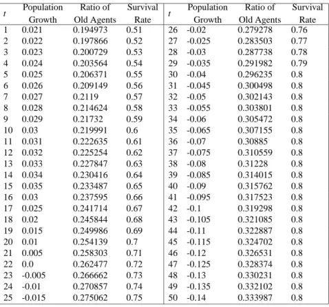
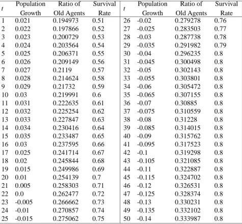
The demographic structure of the economy in our simulation exercises is listed in

Table 1. The population of period t is v

t−1

n

t−1

+ n

t

+ n

t+1

. Although this is an OG

model with two-period lived agents. We treat the generation

t+1

as the children

of generation t when we count population. The justification is that children often

does not have active economic activity, especially the activities of production.

As one can observe that the ratio of old agents in the population increases as t

increases, and the upper bound of the survival rate is 0.8. In our sample economy

the share of old agents in the total population becomes greater and greater as time

increases.

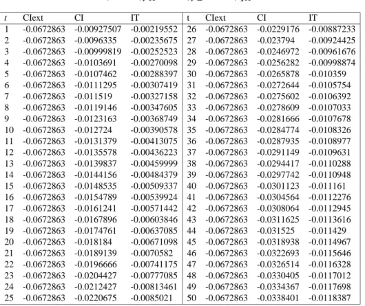
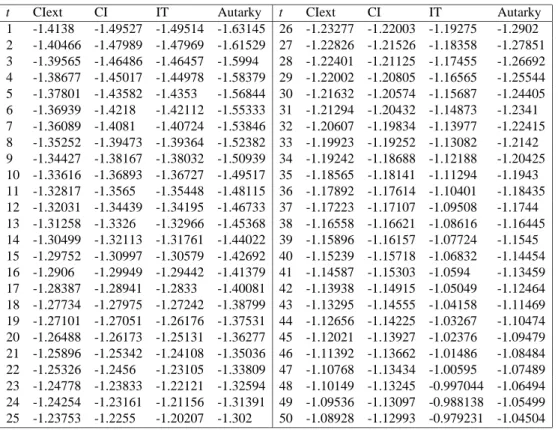
We run simulation for six sets of parameter values

(h, y

H

, y

L

) = (1, 1.5,0.5),

(1, 1, 0.1), (1.01, 1.5, 0.5), (1.01, 1, 0.1), (1.025, 1.5, 0.5), and (1.025, 1, 0.1). The

length of simulation is fifty periods. When a scheme generates greater life time

expected utility, we say it performs better.

-For the case of h

= 1, the CIext scheme performs better than both the CI and

the IT schemes for all simulated periods. The CI scheme performs better than

the IT scheme only for the first three period in the case of

(y

H

, y

L

) = (1.5, 0.5),

while the IT scheme dominates the CI scheme for the rest of periods and for the

all periods in the case of

(y

H

, y

L

) = (1, 0.1).

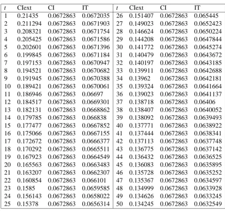
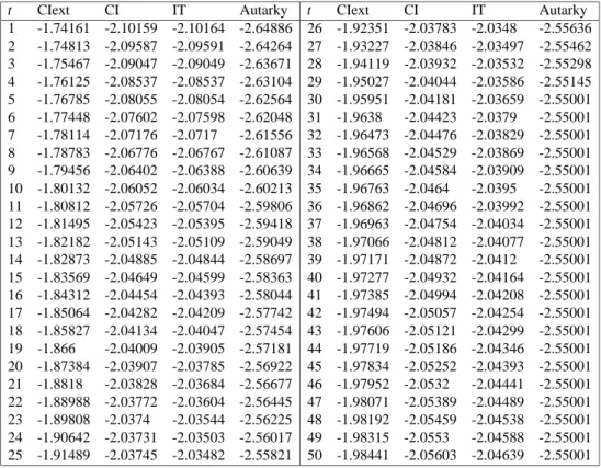
For the case of h

= 1.01 and 1.025, the CIext dominates the CI for the and

the IT schemes for the first many four periods. The IT scheme dominates the CI

scheme almost for all periods.

The following table summarizes some details of the comparison of three schemes.

-The Comparison of Three Schemes

(h, yH, yL) Comparison∗ Periods

(1, 1.5, 0.5) CIext CI for all t CIext IT for all t IT CI for all t (1, 1, 0.1) CIext CI for all t CIext IT for all t CI IT for t= 1, 2, 3

CI= IT for t= 4

(1.01, 1.5, 0.5) CIext CI for t≤ 18

CIext IT for t≤ 16

CIext is incentive incompatible for t≥ 38

CI= IT for all t (1.01, 1, 0.1 ) CIext CI for t≤ 24

CIext IT for t≤ 24

CIext is incentive incompatible for t≥ 75

It CI for t≤ 2

(1.025, 1.5, 0.5) CIext CI for t≤ 12

CIext IT for t≤ 11

CIext is incentive incompatible for t≥ 25

IT CI for t≤ 2

(1.025, 1, 0.1) CIext CI for t≤ 14

CIext IT for t≤ 15

CIext is incentive incompatible for t≥ 40

IT CI for t≤ 3

∗_{: performs better than}

As one can observe from the table, when the economy grows faster, the

num-ber of the periods in which the CIext dominates the IT becomes smallers, that is

as the economy grows, the IT scheme tends to perform betters. The greater y

H

and

y

L

are, the number of periods in which the CIext dominates CI and IT becomes

smaller.

As population aging, the young agent’s burden is heavier and heavier to

main1st year 13

-tain the old age consumption at a constant level. The CIext scheme is designed to

maximize the old agent’s expected utility, while the IT scheme is designed to

max-imize the young agent’s expected utility. As population aging, the CIext scheme

tends to be more costly for the young agents, and thus the young agent will be in

favor of the IT scheme.

Moreover, when the economy grows, the CIext scheme becomes incentive

incompatible for the young agent workable after some certain periods.

4

Concluding Remarks

In an overlapping generation model with aggregate shocks and aging population, I

compare three schemes of intergenerational resource-sharing and study how

eco-nomic growth and population aging interact and how they affect the agent’s

wel-fare.

All schemes conduct intergenerational transfers of resources with different

goals. The intergenerational transfer scheme (IT) aims to maximize the agent’s

lifetime expected utility. The complete insurance against old-consumption scheme

(CI) aims to maximize the expected utility of old agents in the current period by

keeping the old-age consumption constant. The CIext scheme modifies the CI

scheme by retaining some resources from the old age consumption.

I simulate the model with different sets of parameter values. In the set of

parameter values with no productivity growth of the risky technology (h

= 1)

CIext performs better than both IT and CI for all periods. As aggregate shocks

becomes greater (greater y

H

and y

L

), CIext becomes less appealing because it

perform worse than the IT scheme as time increases; comparing with CI, CIext

1st year 14

-performs better than CI in the first many periods and then -performs worse than

CI.

We also extend the model to incorporate productivity growth and find out that

the CI scheme becomes infeasible after twenty periods; the IT scheme performs

better than CI scheme in all fifty periods.

-References

Allen, Franklin and Douglas Gale, “Financial Markets, Intermediaries, and

In-tertemporal Smoothing,” Journal of Political Economy, June 1997, 105 (3),

523–46.

Barr, Nicholas, “Pensions: Overview of the Issues,” Oxford Review of Economic

Policy, Spring 2006, 22 (1), 1–14.

and Peter Diamond, “The Economics of Pensions,” Oxford Review of

Eco-nomic Policy, Spring 2006, 22 (1), 15–39.

Bohn, Henning, “Retirement Savings in an Aging Society: A Case for

Inno-vative Government Debt Management,” University of California at Santa

Bar-bara, Economics Working Paper Series wp3-01, Department of Economics, UC

Santa Barbara April 2001.

Campbell, John Y. and Yves Nosbusch, “Intergenerational risksharing and

equi-librium asset prices,” Journal of Monetary Economics, November 2007, 54 (8),

2251–2268.

Chiang, Yeong-Yuh and You-Ching Yeh, “Aggregate Shocks, Intergenerational

Risk Sharing, and Financial Intermediaries,” Working Paper, Dept. of Money

and Banking, National Chengchi University 2008.

Demange, Gabrielle, “On optimality in intergenerational risk sharing,” Economic

Theory, 2002, 20 (1), 1–27.

-Fehr, Hans, Christian Habermann, and Fabian Kindermann, “Social

Secu-rity with Rational and Hyperbolic Consumers,” Review of Economic Dynamics,

October 2008, 11 (4), 884–903.

Hong, Jay H. and Jose-Victor Rios-Rull, “Social security, life insurance and

annuities for families,” Journal of Monetary Economics, January 2007, 54 (1),

118–140.

- 

 

 

 

Appendix 

 

Tables and Graphs from Simulation 

Table 1: The Demographic Structure

w

= 1, h = 1, y

H

= 1.5, y

L

= 0.5, q

H

= 0.5

t Population Growth Ratio of Old Agents Survival Rate 1 0.021 0.194973 0.51 2 0.022 0.197866 0.52 3 0.023 0.200729 0.53 4 0.024 0.203564 0.54 5 0.025 0.206371 0.55 6 0.026 0.209149 0.56 7 0.027 0.2119 0.57 8 0.028 0.214624 0.58 9 0.029 0.21732 0.59 10 0.03 0.219991 0.6 11 0.031 0.222635 0.61 12 0.032 0.225254 0.62 13 0.033 0.227847 0.63 14 0.034 0.230416 0.64 15 0.035 0.233487 0.65 16 0.03 0.237595 0.66 17 0.025 0.241714 0.67 18 0.02 0.245844 0.68 19 0.015 0.249986 0.69 20 0.01 0.254139 0.7 21 0.005 0.258303 0.71 22 0.0 0.262477 0.72 23 -0.005 0.266662 0.73 24 -0.01 0.270857 0.74 25 -0.015 0.275062 0.75 t Population Growth Ratio of Old Agents Survival Rate 26 -0.02 0.279278 0.76 27 -0.025 0.283503 0.77 28 -0.03 0.287738 0.78 29 -0.035 0.291982 0.79 30 -0.04 0.296235 0.8 31 -0.045 0.300498 0.8 32 -0.05 0.302143 0.8 33 -0.055 0.303801 0.8 34 -0.06 0.305472 0.8 35 -0.065 0.307155 0.8 36 -0.07 0.30885 0.8 37 -0.075 0.310559 0.8 38 -0.08 0.31228 0.8 39 -0.085 0.314015 0.8 40 -0.09 0.315762 0.8 41 -0.095 0.317523 0.8 42 -0.1 0.319298 0.8 43 -0.105 0.321085 0.8 44 -0.11 0.322887 0.8 45 -0.115 0.324702 0.8 46 -0.12 0.326531 0.8 47 -0.125 0.328374 0.8 48 -0.13 0.330231 0.8 49 -0.135 0.332102 0.8 50 -0.14 0.333987 0.8

Table 2: Expected Utility

w

= 1, h = 1, y

H

= 1.5, y

L

= 0.5, q

H

= 0.5

t CIext CI IT Autarky 1 -1.67268 -1.75476 -1.75473 -1.81974 2 -1.66952 -1.74873 -1.74869 -1.81353 3 -1.66656 -1.74299 -1.74294 -1.80759 4 -1.66379 -1.73753 -1.73747 -1.80193 5 -1.66121 -1.73235 -1.73227 -1.79653 6 -1.65881 -1.72742 -1.72732 -1.79137 7 -1.65658 -1.72275 -1.72263 -1.78645 8 -1.65452 -1.71831 -1.71816 -1.78176 9 -1.65262 -1.7141 -1.71393 -1.77728 10 -1.65088 -1.71012 -1.70991 -1.77301 11 -1.64928 -1.70635 -1.7061 -1.76894 12 -1.64784 -1.70278 -1.7025 -1.76507 13 -1.64653 -1.69942 -1.69909 -1.76137 14 -1.64536 -1.69624 -1.69586 -1.75786 15 -1.64432 -1.69326 -1.69282 -1.75451 16 -1.64355 -1.69052 -1.69001 -1.75133 17 -1.64292 -1.68798 -1.68738 -1.7483 18 -1.64242 -1.68561 -1.68492 -1.74543 19 -1.64206 -1.68342 -1.68262 -1.7427 20 -1.64183 -1.6814 -1.68047 -1.74011 21 -1.64173 -1.67955 -1.67848 -1.73766 22 -1.64176 -1.67786 -1.67664 -1.73533 23 -1.64192 -1.67634 -1.67494 -1.73313 24 -1.6422 -1.67498 -1.67339 -1.73105 25 -1.6426 -1.67377 -1.67196 -1.72909 t CIext CI IT Autarky 26 -1.64312 -1.67272 -1.67067 -1.72724 27 -1.64377 -1.67182 -1.6695 -1.7255 28 -1.64453 -1.67108 -1.66846 -1.72387 29 -1.64541 -1.67048 -1.66754 -1.72233 30 -1.64641 -1.67004 -1.66673 -1.7209 31 -1.6477 -1.67089 -1.6671 -1.7209 32 -1.64798 -1.67107 -1.66722 -1.7209 33 -1.64827 -1.67126 -1.66733 -1.7209 34 -1.64856 -1.67145 -1.66745 -1.7209 35 -1.64886 -1.67165 -1.66756 -1.7209 36 -1.64916 -1.67184 -1.66768 -1.7209 37 -1.64946 -1.67205 -1.6678 -1.7209 38 -1.64977 -1.67225 -1.66792 -1.7209 39 -1.65009 -1.67246 -1.66804 -1.7209 40 -1.65041 -1.67267 -1.66816 -1.7209 41 -1.65074 -1.67289 -1.66829 -1.7209 42 -1.65107 -1.67311 -1.66842 -1.7209 43 -1.65141 -1.67333 -1.66854 -1.7209 44 -1.65175 -1.67355 -1.66867 -1.7209 45 -1.6521 -1.67379 -1.6688 -1.7209 46 -1.65245 -1.67402 -1.66893 -1.7209 47 -1.65281 -1.67426 -1.66907 -1.7209 48 -1.65318 -1.6745 -1.6692 -1.7209 49 -1.65356 -1.67475 -1.66934 -1.7209 50 -1.65394 -1.675 -1.66948 -1.7209

Table 3: Young Losses in Welfare

w

= 1, h = 1, y

H

= 1.5, y

L

= 0.5, q

H

= 0.5

t CIext CI IT 1 -0.0672863 -0.00927507 -0.00219552 2 -0.0672863 -0.0096335 -0.00235675 3 -0.0672863 -0.00999819 -0.00252523 4 -0.0672863 -0.0103691 -0.00270098 5 -0.0672863 -0.0107462 -0.00288397 6 -0.0672863 -0.0111295 -0.00307419 7 -0.0672863 -0.011519 -0.00327158 8 -0.0672863 -0.0119146 -0.00347605 9 -0.0672863 -0.0123163 -0.00368749 10 -0.0672863 -0.012724 -0.00390578 11 -0.0672863 -0.0131379 -0.00413075 12 -0.0672863 -0.0135578 -0.00436223 13 -0.0672863 -0.0139837 -0.00459999 14 -0.0672863 -0.0144156 -0.00484379 15 -0.0672863 -0.0148535 -0.00509337 16 -0.0672863 -0.0154789 -0.00539924 17 -0.0672863 -0.0161241 -0.00571442 18 -0.0672863 -0.0167896 -0.00603846 19 -0.0672863 -0.0174761 -0.00637085 20 -0.0672863 -0.018184 -0.00671098 21 -0.0672863 -0.0189139 -0.0070582 22 -0.0672863 -0.0196666 -0.00741175 23 -0.0672863 -0.0204427 -0.00777085 24 -0.0672863 -0.0212427 -0.00813461 25 -0.0672863 -0.0220675 -0.0085021 t CIext CI IT 26 -0.0672863 -0.0229176 -0.00887233 27 -0.0672863 -0.023794 -0.00924425 28 -0.0672863 -0.0246972 -0.00961676 29 -0.0672863 -0.0256282 -0.00998874 30 -0.0672863 -0.0265878 -0.010359 31 -0.0672863 -0.0272644 -0.0105754 32 -0.0672863 -0.0275602 -0.0106392 33 -0.0672863 -0.0278609 -0.0107033 34 -0.0672863 -0.0281666 -0.0107678 35 -0.0672863 -0.0284774 -0.0108326 36 -0.0672863 -0.0287935 -0.0108977 37 -0.0672863 -0.0291149 -0.0109631 38 -0.0672863 -0.0294417 -0.0110288 39 -0.0672863 -0.0297742 -0.0110948 40 -0.0672863 -0.0301123 -0.011161 41 -0.0672863 -0.0304564 -0.0112276 42 -0.0672863 -0.0308064 -0.0112945 43 -0.0672863 -0.0311625 -0.0113616 44 -0.0672863 -0.031525 -0.011429 45 -0.0672863 -0.0318938 -0.0114967 46 -0.0672863 -0.0322693 -0.0115646 47 -0.0672863 -0.0326514 -0.0116328 48 -0.0672863 -0.0330405 -0.0117012 49 -0.0672863 -0.0334367 -0.0117698 50 -0.0672863 -0.0338401 -0.0118387

Table 4: Old Gains in Welfare

w

= 1, h = 1, y

H

= 1.5, y

L

= 0.5, q

H

= 0.5

t CIext CI IT 1 0.21435 0.0672863 0.0672035 2 0.211294 0.0672863 0.0671903 3 0.208321 0.0672863 0.0671754 4 0.205425 0.0672863 0.0671586 5 0.202601 0.0672863 0.0671396 6 0.199845 0.0672863 0.0671184 7 0.197153 0.0672863 0.0670947 8 0.194521 0.0672863 0.0670682 9 0.191945 0.0672863 0.0670388 10 0.189421 0.0672863 0.0670061 11 0.186946 0.0672863 0.06697 12 0.184517 0.0672863 0.0669301 13 0.182131 0.0672863 0.0668862 14 0.179785 0.0672863 0.066838 15 0.177477 0.0672863 0.0667852 16 0.175066 0.0672863 0.0667155 17 0.172672 0.0672863 0.0666377 18 0.170292 0.0672863 0.0665511 19 0.167923 0.0672863 0.0664549 20 0.165563 0.0672863 0.0663483 21 0.163207 0.0672863 0.0662307 22 0.160854 0.0672863 0.066101 23 0.1585 0.0672863 0.0659585 24 0.156143 0.0672863 0.0658022 25 0.15378 0.0672863 0.0656314 t CIext CI IT 26 0.151407 0.0672863 0.065445 27 0.149023 0.0672863 0.0652423 28 0.146624 0.0672863 0.0650224 29 0.144208 0.0672863 0.0647844 30 0.141772 0.0672863 0.0645274 31 0.140479 0.0672863 0.0643672 32 0.140197 0.0672863 0.0643185 33 0.139911 0.0672863 0.0642688 34 0.13962 0.0672863 0.0642181 35 0.139324 0.0672863 0.0641664 36 0.139023 0.0672863 0.0641137 37 0.138718 0.0672863 0.06406 38 0.138407 0.0672863 0.0640052 39 0.138092 0.0672863 0.0639493 40 0.137771 0.0672863 0.0638922 41 0.137444 0.0672863 0.0638341 42 0.137113 0.0672863 0.0637748 43 0.136775 0.0672863 0.0637142 44 0.136432 0.0672863 0.0636525 45 0.136083 0.0672863 0.0635895 46 0.135728 0.0672863 0.0635252 47 0.135367 0.0672863 0.0634597 48 0.134999 0.0672863 0.0633928 49 0.134626 0.0672863 0.0633245 50 0.134245 0.0672863 0.0632549

Table 5: The Demographic Structure

w

= 1, h = 1, y

H

= 1, y

L

= 0.1, q

H

= 0.5

t Population Growth Ratio of Old Agents Survival Rate 1 0.021 0.194973 0.51 2 0.022 0.197866 0.52 3 0.023 0.200729 0.53 4 0.024 0.203564 0.54 5 0.025 0.206371 0.55 6 0.026 0.209149 0.56 7 0.027 0.2119 0.57 8 0.028 0.214624 0.58 9 0.029 0.21732 0.59 10 0.03 0.219991 0.6 11 0.031 0.222635 0.61 12 0.032 0.225254 0.62 13 0.033 0.227847 0.63 14 0.034 0.230416 0.64 15 0.035 0.233487 0.65 16 0.03 0.237595 0.66 17 0.025 0.241714 0.67 18 0.02 0.245844 0.68 19 0.015 0.249986 0.69 20 0.01 0.254139 0.7 21 0.005 0.258303 0.71 22 0.0 0.262477 0.72 23 -0.005 0.266662 0.73 24 -0.01 0.270857 0.74 25 -0.015 0.275062 0.75 t Population Growth Ratio of Old Agents Survival Rate 26 -0.02 0.279278 0.76 27 -0.025 0.283503 0.77 28 -0.03 0.287738 0.78 29 -0.035 0.291982 0.79 30 -0.04 0.296235 0.8 31 -0.045 0.300498 0.8 32 -0.05 0.302143 0.8 33 -0.055 0.303801 0.8 34 -0.06 0.305472 0.8 35 -0.065 0.307155 0.8 36 -0.07 0.30885 0.8 37 -0.075 0.310559 0.8 38 -0.08 0.31228 0.8 39 -0.085 0.314015 0.8 40 -0.09 0.315762 0.8 41 -0.095 0.317523 0.8 42 -0.1 0.319298 0.8 43 -0.105 0.321085 0.8 44 -0.11 0.322887 0.8 45 -0.115 0.324702 0.8 46 -0.12 0.326531 0.8 47 -0.125 0.328374 0.8 48 -0.13 0.330231 0.8 49 -0.135 0.332102 0.8 50 -0.14 0.333987 0.8

Table 6: Expected Utility

w

= 1, h = 1, y

H

= 1, y

L

= 0.1, q

H

= 0.5

t CIext CI IT Autarky 1 -1.74161 -2.10159 -2.10164 -2.64886 2 -1.74813 -2.09587 -2.09591 -2.64264 3 -1.75467 -2.09047 -2.09049 -2.63671 4 -1.76125 -2.08537 -2.08537 -2.63104 5 -1.76785 -2.08055 -2.08054 -2.62564 6 -1.77448 -2.07602 -2.07598 -2.62048 7 -1.78114 -2.07176 -2.0717 -2.61556 8 -1.78783 -2.06776 -2.06767 -2.61087 9 -1.79456 -2.06402 -2.06388 -2.60639 10 -1.80132 -2.06052 -2.06034 -2.60213 11 -1.80812 -2.05726 -2.05704 -2.59806 12 -1.81495 -2.05423 -2.05395 -2.59418 13 -1.82182 -2.05143 -2.05109 -2.59049 14 -1.82873 -2.04885 -2.04844 -2.58697 15 -1.83569 -2.04649 -2.04599 -2.58363 16 -1.84312 -2.04454 -2.04393 -2.58044 17 -1.85064 -2.04282 -2.04209 -2.57742 18 -1.85827 -2.04134 -2.04047 -2.57454 19 -1.866 -2.04009 -2.03905 -2.57181 20 -1.87384 -2.03907 -2.03785 -2.56922 21 -1.8818 -2.03828 -2.03684 -2.56677 22 -1.88988 -2.03772 -2.03604 -2.56445 23 -1.89808 -2.0374 -2.03544 -2.56225 24 -1.90642 -2.03731 -2.03503 -2.56017 25 -1.91489 -2.03745 -2.03482 -2.55821 t CIext CI IT Autarky 26 -1.92351 -2.03783 -2.0348 -2.55636 27 -1.93227 -2.03846 -2.03497 -2.55462 28 -1.94119 -2.03932 -2.03532 -2.55298 29 -1.95027 -2.04044 -2.03586 -2.55145 30 -1.95951 -2.04181 -2.03659 -2.55001 31 -1.9638 -2.04423 -2.0379 -2.55001 32 -1.96473 -2.04476 -2.03829 -2.55001 33 -1.96568 -2.04529 -2.03869 -2.55001 34 -1.96665 -2.04584 -2.03909 -2.55001 35 -1.96763 -2.0464 -2.0395 -2.55001 36 -1.96862 -2.04696 -2.03992 -2.55001 37 -1.96963 -2.04754 -2.04034 -2.55001 38 -1.97066 -2.04812 -2.04077 -2.55001 39 -1.97171 -2.04872 -2.0412 -2.55001 40 -1.97277 -2.04932 -2.04164 -2.55001 41 -1.97385 -2.04994 -2.04208 -2.55001 42 -1.97494 -2.05057 -2.04254 -2.55001 43 -1.97606 -2.05121 -2.04299 -2.55001 44 -1.97719 -2.05186 -2.04346 -2.55001 45 -1.97834 -2.05252 -2.04393 -2.55001 46 -1.97952 -2.0532 -2.04441 -2.55001 47 -1.98071 -2.05389 -2.04489 -2.55001 48 -1.98192 -2.05459 -2.04538 -2.55001 49 -1.98315 -2.0553 -2.04588 -2.55001 50 -1.98441 -2.05603 -2.04639 -2.55001