中國城市不動產價格泡沫之探討 - 政大學術集成

全文

(1)國立政治大學地政學系碩士論文私立中國地政研究所. 政治大中國城市不動產價格泡沫之探討立 ‧. ‧ 國. 學. China’s Housing Bubbles and the Driving Factors. n. er. io. sit. y. Nat. al. 西. 元. Ch. engchi. 研究生：. 黃. 指導教授：. 林左裕. 二. 〇. 一. i n U. v. 斐博士. 四. 年. 七. 月.

(2) 謝誌. 時光匆匆，這段到台灣求學的旅程一眨眼就將近尾聲。兩年的研究所生活，或苦或甜，或哭或笑，都磨練了我獨立作業的研究能力以及不畏艱難的意志。這過程中，太多人給予我鼓勵與幫助，遺憾不能一一當面道謝，就讓我在這裡細細記錄這份對大家的感激。首先要感謝我的指導教授林左裕老師，兩年來在學習與論文上都給予細心教導，在確定論文題目以及收集數據過程中提供方向，當論文寫作遇到困難時老師還會幫助我釐清思路。老師也經常鼓勵我參加研討會以及論文比賽，不僅讓我. 政治大. 收穫不少論文修改意見，還鍛煉了我的膽量以及簡報能力。另外，感謝我的口委彭建文老師和林哲群老師，您們寶貴的建議使我的論文更嚴謹、完備。謝謝張金. 立. 鶚老師、陳奉瑤老師、林森田老師、丁秀吟老師、蔡育新老師、張鈺光老師、孫. ‧ 國. 學. 振義老師、吳家昌老師，您們的課堂增進了我的專業知識，獲益良多。還要感謝江穎慧老師、筱蓉學姐、瑋玲學姐，在期初、期末報告評論我的論文，讓我找到. ‧. 論文改進的方向。. y. Nat. 接著要感謝研究所的同學們這兩年來對我的照顧。可愛活潑的宜均、美麗. sit. 大方的雪芬，感謝你們平時一直聽我傾訴、陪我玩耍，讓我能夠重新恢復活力。. al. er. io. 還有平時對我也照顧有加的葛仲、阿香、Kelly、孟瑄、錚錚、佳萱、俊叡、宗. n. v i n Ch 帶我遊歷台灣、品嘗美食。謝謝左家學弟妹虹荏、佑倫、家寶平日給予的幫助， engchi U 很開心能與你們一起奮鬥。特別感謝我的未婚夫宇均，無論發生什麼事都給予我軒、菜米、浩學、飛利浦、蒂蒂、珍珠、芳儀、豐荃、宇璇、亭均等，謝謝你們. 鼓勵與支持。最後要感謝爸爸媽媽支持我繼續求學的決定，沒有你們默默的付出也就沒有我今天的成績。回首與大家從陌生到熟悉的這兩年時光，心裡湧現很多道別的話語，但似乎說出來就沒有了味道。我們同行過的這段難忘旅程，會永遠生長在我的記憶裡。感謝大家這兩年來陪伴我、幫助我、包容我，希望我也給你們帶來過同樣的快樂！親愛的大家，感謝！再見！黃斐. 謹誌於綜院六樓研究室 2014 年 7 月.

(3) 摘要. 隨著中國大陸經濟的高度成長，不動產市場也隨之發展。在貸款利率及不動產相關稅負長期偏低之下，住宅產品的投資需求不斷上升，使得房價一路高漲。房屋價格的增幅過大、增速過高，已經超出了合理的範圍。截至 2010 年，中國大陸推出一系列以抑制房價為主要目的的宏觀調控政策，許多重點城市也陸續推出以“限購令”為主要內容的地方性政策來調控不動產市場。由於中國大陸地幅遼闊，各地的不動產市場因受各種因素影響而發展各異，因此挑選了北京、上海、廣州三個頗具代表性的重點城市作為研究對象。本文應用年租金與加權平均資本成本（WACC）還原基本價值，以其與市場價格間的差距作為泡沫程度的估計，. 政治大. 計算出這三個城市 2007 年至 2012 年間不動產價格泡沫程度。藉由這三個城市的不動產市場泡沫狀況，運用共整合分析檢視中國城市不動產價格泡沫的影響因素，. 立. 并以 Granger 因果關係檢定探討三地不動產價格泡沫與各因素之領先落後關係。. ‧ 國. 學. 實證結果顯示，人均可支配收入和金融機構各項信貸總額對不動產價格泡. ‧. 沫具有正向影響，不動產價格泡沫則對其本身具有負向影響，而抵押貸款利率與不動產價格泡沫先是正相關而後轉為負相關的關係。而根據 Granger 因果關係檢. y. Nat. 定結果，北京不動產價格泡沫落後於金融機構各項貸款總額，而上海不動產價格. io. 押貸款利率與金融機構各項貸款總額。. n. al. Ch. engchi. er. sit. 泡沫領先於人均可支配收入，廣州不動產價格泡沫則落後於人均可支配收入、抵. i n U. 關鍵詞：不動產價格泡沫、基本價值、資本還原率. v.

(4) Abstract With the rapid economic development in China, the real estate market has been undergoing a great boom. The low interest and tax rates are very favorable for the continuously increasing house demands, and thus resulting in higher housing prices. And the extremely rapidly increasing housing prices are not reasonable. Until 2010, Chinese government had published a series of national housing regulatory decisions to address the over-heating real estate market. And the restrictions on house purchase have been put into practice in some major cities. Given that China has a vast territory with large variety, the impact of these regulations on the local real estate markets of the cities can hardly be determined. Therefore, we study here the real estate market in. 政治大 China. This study evaluates the housing bubbles situations in these cities from 2007 to 立 Beijing, Shanghai and Guangzhou, three of the most representative major cities in. 2012 by comparing fundamental values with market prices. The fundamental value of. ‧ 國. 學. real estate can be calculated by annual rents and WACC. Based on the evaluated housing bubbles situations, this study then applies Cointegration analysis to further. ‧. explore the factors that may contribute to China’s housing bubbles. In addition, Granger causality test is employed to examine the lead/lag relationship between. y. Nat. er. io. al. sit. housing bubbles and the variables.. n. The empirical result shows that per-capita disposable incomes and total loans of. Ch. i n U. v. financial institutions are positively related to China’s housing bubbles. And the. engchi. housing bubbles in these three cities are negatively related to themselves. In addition, the impact of interest rates on housing bubbles is positive and later turns negative with respect to the magnitude of increasing rates. According to the results of Granger causality tests, Beijing’s housing bubbles are Granger caused by total loans while property bubbles in Shanghai lead personal incomes. Furthermore, housing bubbles in Guangzhou are Granger caused by personal disposable incomes, interest rates and total loans.. Key Words: Housing Bubble, Fundamental Value, Capitalization Rate.

(5) China’s Housing Bubbles and the Driving Factors. Context Chapter 1 Introduction................................................................................................ 1 1.1 General Background and Research Motivation ............................................................... 1 1.2 Research Method and Scope ........................................................................................... 5 1.3 Research Overview .......................................................................................................... 7. Chapter 2 Literature Review ...................................................................................... 9 2.1 The Definition of the “Bubble” ....................................................................................... 9 2.2 The Measure of Housing Bubbles ................................................................................. 11 2.3 Review of Housing Bubble Factors ............................................................................... 14. 政治大 3.1 Research Method ........................................................................................................... 17 立 3.2 Data Information ........................................................................................................... 23. Chapter 3 Research Method and Data Information ............................................... 17. ‧ 國. 學. Chapter 4 Measure of Housing Bubbles .................................................................. 26 4.1 Trends of Housing Prices and Rents ............................................................................. 26. ‧. 4.2 Fundamental Value........................................................................................................ 29. sit. y. Nat. 4.3 Status of Housing Bubbles ............................................................................................ 32. io. er. Chapter 5 Empirical Results ..................................................................................... 35 5.1 Structural Change .......................................................................................................... 35. n. al. Ch. i n U. v. 5.2 Unit Root Test ............................................................................................................... 38. engchi. 5.3 Cointegration Test ......................................................................................................... 39 5.4 Vector Error Correction Model ..................................................................................... 41 5.5 Granger Causality Test .................................................................................................. 46. Chapter 6 Conclusions and Discussion .................................................................... 48 6.1 Conclusions ................................................................................................................... 48 6.2 Suggestions.................................................................................................................... 51 6.3 Limitations..................................................................................................................... 53. References ................................................................................................................... 54. I.

(6) China’s Housing Bubbles and the Driving Factors. List of Figures Figure 1- 1 China’s Housing Sales Area and the Real Estate Development .................. 1 Figure 1- 2 The House Price-to-Income Ratios in Beijing, Shanghai and Guangzhou . 2 Figure 1- 3 The Research Process .................................................................................. 8 Figure 3- 1 Process of Research Method ..................................................................... 18 Figure 4- 1 The Housing Prices in Beijing, Shanghai and Guangzhou ....................... 27 Figure 4- 2 The Housing Rents in Beijing, Shanghai and Guangzhou ........................ 27 Figure 4- 3 The Market Capitalization Rates in Beijing, Shanghai and Guangzhou ... 28 Figure 4- 4 The 5-year deposit rates and the 5-year loan rates .................................... 30. 政治大. Figure 4- 5 The Fundamental Values in Beijing, Shanghai and Guangzhou (50% LTV) ...................................................................................................................................... 30. 立. ‧ 國. 學. Figure 4- 6 The Fundamental Values in Beijing, Shanghai and Guangzhou (70% LTV) ...................................................................................................................................... 31 Figure 4- 7 The Housing Bubbles in Beijing, Shanghai and Guangzhou (50% LTV) . 32. ‧. Figure 4- 8 The Housing Bubbles in Beijing, Shanghai and Guangzhou (70% LTV) . 33 Figure 5- 1 Result of CUSUM Test for BJ................................................................... 36. y. Nat. sit. Figure 5- 2 Result of CUSUM Test for SH .................................................................. 36. er. io. Figure 5- 3 Result of CUSUM Test for GZ ................................................................. 37. al. n. v i n C h in Beijing, Shanghai Figure 5- 5 The employed population e n g c h i U and Guangzhou .............. 45 Figure 5- 4 The population in Beijing, Shanghai and Guangzhou............................... 45. II.

(7) China’s Housing Bubbles and the Driving Factors. List of Tables Table 3- 1 The Variable Descriptions ........................................................................... 24 Table 3- 2 Descriptive Statistics of Variables .............................................................. 25 Table 5- 1 Result of Unit Root Test ............................................................................. 38 Table 5- 2 The Optimal Lag Order............................................................................... 39 Table 5- 3 Results of Cointegration Test ...................................................................... 40 Table 5- 4 VECM Analysis on INCOME_BJ, LOAN, INT and BJ ............................ 43 Table 5- 5 VECM Analysis on INCOME_SH, LOAN, INT and SH ........................... 43 Table 5- 6 VECM Analysis on INCOME_GZ, LOAN, INT and GZ .......................... 44. 政治大 Table 5- 8 Granger Causality Test on INCOME_SH, LOAN, INT and SH ................ 47 立 Table 5- 9 Granger Causality Test on INCOME_GZ, LOAN, INT and GZ ................ 47 Table 5- 7 Granger Causality Test on INCOME_BJ, LOAN, INT and BJ .................. 47. ‧. ‧ 國. 學. n. er. io. sit. y. Nat. al. Ch. engchi. III. i n U. v.

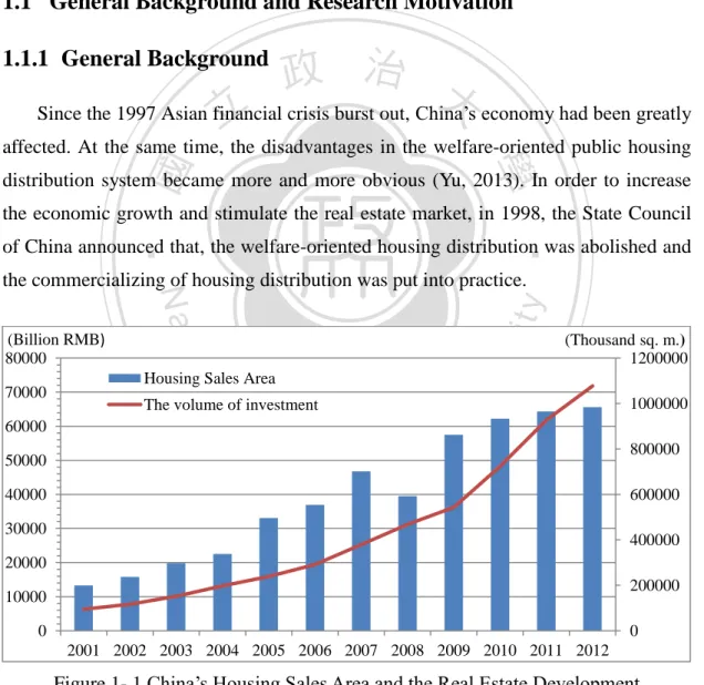
(8) China’s Housing Bubbles and the Driving Factors. Chapter 1 Introduction This chapter is divided into three parts. The first part mainly introduces the general background and research motivation of this study. Then, the research method and scope are described in the second part. The final part presents the research framework and process.. 1.1 General Background and Research Motivation. 政治大 Since the 1997 Asian financial 立 crisis burst out, China’s economy had been greatly. 1.1.1 General Background. affected. At the same time, the disadvantages in the welfare-oriented public housing. ‧ 國. 學. distribution system became more and more obvious (Yu, 2013). In order to increase the economic growth and stimulate the real estate market, in 1998, the State Council. ‧. of China announced that, the welfare-oriented housing distribution was abolished and. y. sit. al. er. io. (Billion RMB) 80000. Nat. the commercializing of housing distribution was put into practice.. n. Housing Sales Area. 70000. Ch. The volume of investment. 60000 50000. engchi. i n U. (Thousand sq. m.) 1200000. v. 40000. 1000000 800000 600000. 30000. 400000. 20000 200000. 10000 0. 0 2001 2002 2003 2004 2005 2006 2007 2008 2009 2010 2011 2012. Figure 1- 1 China’s Housing Sales Area and the Real Estate Development Source: CSMAR From then on, the real estate market in China has been undergoing a great boom. From 2001 to 2012, the housing sales area rose from 199387.5 thousand square 1.

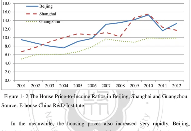
(9) China’s Housing Bubbles and the Driving Factors. meters to 984675.13 thousand square meters, an increase of 393.85 percent. Besides, the real estate development climbed from ￥6344.11 billion to ￥71803.79 billion, increasing 1031.82 percent (as shown in Figure 1-1). The rapid growth of the real estate market stimulated the economic growth. Furthermore, the real estate industry became one of the pillar industries in the domestic economy. 18.0. Beijing. 16.0. Shanghai. 14.0. Guangzhou. 12.0 10.0 8.0 6.0. 立. 4.0. 2001. 2002. 2003. 2004. 2005. 2006. 2007. 2008. 學. 0.0. ‧ 國. 2.0. 政治大 2009. 2010. 2011. 2012. ‧. Figure 1- 2 The House Price-to-Income Ratios in Beijing, Shanghai and Guangzhou Source: E-house China R&D Institute. sit. y. Nat. In the meanwhile, the housing prices also increased very rapidly. Beijing,. io. n. al. er. Shanghai and Guangzhou rank among the priciest housing markets in the world,. i n U. v. based on calculations by the International Monetary Fund (Quartz, 2013). In the study. Ch. engchi. of E-house China R&D Institute, the house price-to-income ratios 1 in Beijing, Shanghai and Guangzhou from 2001 to 2012 showed a marked increase. As reported in Figure 1-2, the house price-to-income ratio in Beijing increased from 9.5 to 13.3 while Shanghai’s price-to-income ratio climbed from 6.7 to 11.7. And the price-to-income in Guangzhou rose from 5.0 to 9.9. High price-to-income ratios reflect that the houses in these three cities might be out of most people’s price ranges. Further, the high housing price would place an intolerable burden on home buyers. If the high housing price is mainly comprised by bubbles, it will threaten the steady development of the domestic economy. Once the housing bubbles burst, the home. 1. The house price-to-income ratio measures housing prices in a given city against disposable incomes, which reflects people’s housing affordability. The formula of price-to-income ratio in this study is written as follows. 𝐻𝑜𝑢𝑠𝑖𝑛𝑔 𝑃𝑟𝑖𝑐𝑒× 𝑃𝑒𝑟−𝑐𝑎𝑝𝑖𝑡𝑎 𝑅𝑒𝑠𝑖𝑑𝑒𝑛𝑡𝑖𝑎𝑙 𝐴𝑟𝑒𝑎 House Price to Income Ratio = 𝑃𝑒𝑟−𝑐𝑎𝑝𝑖𝑡𝑎 𝐷𝑖𝑠𝑝𝑜𝑠𝑎𝑏𝑙𝑒 𝐼𝑛𝑐𝑜𝑚𝑒. 2.

(10) China’s Housing Bubbles and the Driving Factors. buyers’ capital chains are likely to fracture and the financial market liquidity might dry up. By then, it would be very difficult for the entire society to finance. As a result, production and consumption in other industries would slide into stagnation. In the end, it will send China into deep recession. It can be seen from Figure 1-2 that the variations of the house price-to-income ratios in Beijing, Shanghai and Guangzhou have differed from each other since 2007, which were caused by a confluence of factors. Under the impact of the subprime mortgage crisis, the global economy was mired in recession. China's economy was also influenced in 2007. Unemployment rose and the population's willingness to spend money declined. Meanwhile, China’s real estate market was badly hit. Thus the. 治政 moderately easy monetary policies. Credit limits for commercial 大 banks were removed 立 reduced many times. In 2010, the government carried while the mortgage rates were. government unveiled a four trillion yuan stimulus package and decided to adopt. ‧ 國. 學. out a series of stringent regulations which aim to address the over-heating real estate market, including tightening mortgage credit’s standards and blocking migrant buyers. ‧. from owning new houses.. sit. y. Nat. However，the impacts of the economy and housing polices on the local real estate markets of these three cities might be immensely different. Beijing is the capital of. io. er. China and the national political center. Many headquarters of China’s largest. al. n. v i n C h is a global U introduced earliest in Beijing. Shanghai e n g c h i financial center. It has attracted. state-owned companies are based in Beijing. And a number of housing policies were. lots of foreign investments in various industries. Moreover, Shanghai leads the nation. in the development of real estate market. Guangzhou is the largest city in southern China. It is also one of China’s leading commercial and manufacturing regions. Besides, Guangzhou is the first city to develop real estate industry in China. Therefore, this study will focus on the housing bubbles in Beijing, Shanghai and Guangzhou from 2007 to 2012.. 1.1.2 Research Motivation Due to the aftermath of housing bubbles that mentioned above, many scholars were concerned about the problem of housing bubbles in recent years. According to the past researches, there are various methods to judge the housing bubbles, such as 3.

(11) China’s Housing Bubbles and the Driving Factors. using some indicators and building econometric models (Garino and Sarno, 2004; Krainer and Wei, 2004; Hott and Monnin, 2008). But these kinds of methods just judge whether the housing bubbles exist or not. And only few methods can calculate the degree of housing bubbles exactly. Hence it is necessary to create a method that can measure the status of housing bubbles. In order to curb the over-heating investment and stable the housing prices, the Chinese government has put forward on national housing regulations since 2003. The main contents of these housing regulations are curbing speculative investment, increasing housing supply and accelerating the construction of affordable housing projects. Nevertheless the effects are not as significant as expected. So there is a. 治政 can provide suggestions for housing policies. 大立. pressing need for the research on the driving forces of China’s housing bubbles which. ‧ 國. 學. 1.1.3 Research Purpose. Based on the motivation above, the purposes of this research are as follows:. ‧ y. Nat. (1) To measure the status of China’s housing bubbles. This research will define. sit. the concept of the bubble and find out a method which can calculate the degree of. er. io. housing bubbles exactly.. al. n. v i n To explore the factorsCwhich China’s housing bubbles. This study h e naffect gchi U. (2). intends to investigate the equilibrium relationship between China’s housing bubbles and the variables by employing cointegration analysis and Granger Causality test. In addition, this study attempts to provide some suggestions for promoting sustainable and healthy development of China’s real estate market.. 4.

(12) China’s Housing Bubbles and the Driving Factors. 1.2 Research Method and Scope 1.2.1 Research Method (1) Theory and Literature Review First of all, we select the appropriate definition of the bubble from the relevant theories and literatures. Then we sort out the measure of housing bubbles and the driving forces which affect the housing bubbles, according to the past researches. These methods and factors will provide reference for the empirical analysis in this study.. 政治大. (2) Modeling and Empirical Analysis. 立. The empirical modeling analysis is applied to examine the relationship between. ‧ 國. 學. China’s housing bubbles and the factors that are chosen. Through the use of Eviews statistical software, we employ the cointegration test to explore the long-run. ‧. equilibrium relationship. In terms of the short-run dynamics, we use Vector Error Correction Model (VECM) or Vector Autoregressive (VAR) model. Finally, we apply. y. Nat. sit. Granger Causality test to clarify the lead/lag relationship between China’s housing. n. al. er. io. bubbles and the variables.. 1.2.2 Research Scope. Ch. engchi. i n U. v. (1) Research Objects This study tries to explore the relationship between China’s housing bubbles and some variables. However, considering the availability of the data, this study focuses on residential real estate market. So the housing prices and rents in this study mean the ones of residential real estate. (2) Time and Spatial Scope Although the China’s real estate market has developed for more than 10 years, the related data are limited and hard to obtain. Due to the background information above 5.

(13) China’s Housing Bubbles and the Driving Factors. and the limitation of data, the study period ranges from January 2007 to November 2012. Since China has a vast territory, the real estate markets which are influenced by all kinds of factors vary from place to place. With the support of the real economy, real estate in Beijing, Shanghai and Guangzhou has been especially welcomed by investors. And the house markets in these three cities are quite lively. In light of this concern, this study selects Beijing, Shanghai and Guangzhou to discuss.. 立. 政治大. ‧. ‧ 國. 學. n. er. io. sit. y. Nat. al. Ch. engchi. 6. i n U. v.

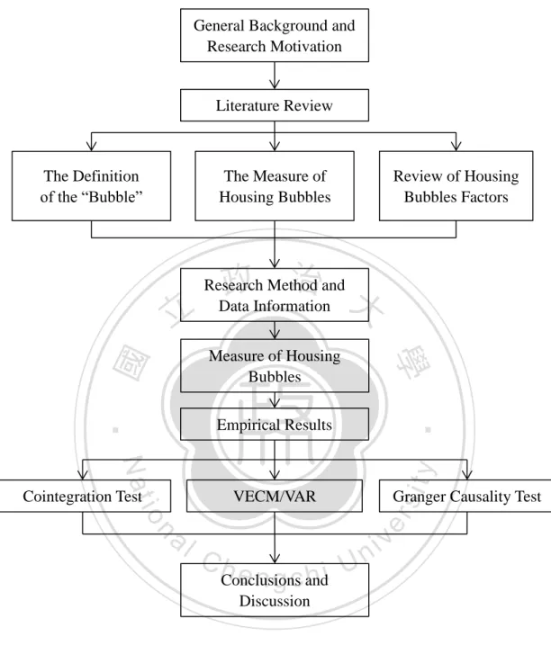
(14) China’s Housing Bubbles and the Driving Factors. 1.3 Research Overview 1.3.1 Research Framework This study consists of six chapters as follows. Chapter 1 is “Introduction”, which mainly contains the general background, research motivation and research purpose. Besides, this part gives a brief introduction to the research scope and research overview of this study. Chapter 2 is “Literature Review”, discussing the definitions of the bubble, the measures of housing bubbles and the factors which influence the housing bubbles. Chapter 3 is “Research Method and Data Information”, presenting the methodology and the data used in this study. Chapter 4 is “Measure of Housing Bubbles”, explaining the status of the housing bubbles in Beijing, Shanghai and. 政治大 and analyses the practical 立 meanings of these results. Chapter 6 is “Conclusions and Guangzhou. Chapter 5 is “Empirical Results”, which illustrates the empirical results. Discussion”, which summarizes the implications of this study and provides. ‧ 國. 學. suggestions for housing policies.. ‧. n. er. io. sit. y. Nat. al. Ch. engchi. 7. i n U. v.

(15) China’s Housing Bubbles and the Driving Factors. 1.3.2 Research Process General Background and Research Motivation. Literature Review. The Definition of the “Bubble”. The Measure of Housing Bubbles. 立. Review of Housing Bubbles Factors. 政治大. Research Method and Data Information. ‧. ‧ 國. 學. Measure of Housing Bubbles Empirical Results. sit. y. Nat. VECM/VAR. io. n. al. Granger Causality Test. er. Cointegration Test. Ch. engchi. Conclusions and Discussion. i n U. Figure 1- 3 The Research Process. 8. v.

(16) China’s Housing Bubbles and the Driving Factors. Chapter 2 Literature Review This chapter mainly reviews the relevant literatures about housing bubbles and is divided into three sections. The first section explores the definition of housing bubbles. The second section discusses the method to measure housing bubbles. At last, the third section explores the relationship between housing bubbles and other factors, as the foundation for the empirical analysis.. 2.1 The Definition of the “Bubble”. 政治大. The researches on asset bubbles are long-standing. And the scholars never stop. 立. investigating the definition of “Bubble”. Stiglitz (1990) indicated that the prices of. ‧ 國. 學. asset would not stop increasing if the investors believed the asset could be sold for a higher price in the future than they had been expecting. In other words, an asset bubble exists when the price is not justified by fundamental factors. Besides, Diba and. ‧. Grossman (1988) pointed out that a rational bubble reflected a self-confirming belief. y. Nat. that an asset’s price depended on a combination of variables that were not part of. io. sit. market fundamentals. In short, an asset bubble could be defined as the difference. er. between the market price and the market fundamental (Tirole, 1985).. al. n. v i n C happlies to real estate. The definition of bubble also e n g c h i U A housing bubble can be described as a deviation of the market price from the fundamental value of the house (Krainer, 2003; Smith et al., 2006). According to this definition, it is possible to quantify the value of housing bubbles. As for the causes of housing bubbles, Levin and Wright (1997a, 1997b) indicated that a house price bubble that could differ between actual and mix-adjusted properties would arise when households could take positions in the market by buying larger or higher quality houses in anticipation of expected price rises. In the theory of housing price proposed by Muellbauer and Murphy (1997), the section that housing prices exceed fundamental values is caused by speculation, which can be defined as speculative prices-i.e. housing bubbles. Briefly speaking, the house purchase for investment makes the price depart from the equilibrium level and then results in housing bubbles.. 9.

(17) China’s Housing Bubbles and the Driving Factors. In summary, it is widely considered that a housing bubble can be defined as the deviation of the market price from the fundamental value of the house. And the later analyses on housing bubbles in this study would employ this definition.. 立. 政治大. ‧. ‧ 國. 學. n. er. io. sit. y. Nat. al. Ch. engchi. 10. i n U. v.

(18) China’s Housing Bubbles and the Driving Factors. 2.2 The Measure of Housing Bubbles According to the definition of housing bubbles above, it is necessary to confirm market prices and fundamental values before gauging the situation of housing bubbles. The housing prices can be obtained directly. But it is complicated to get the fundamental values. In the past literature, there are lots of methods to calculate the house fundamental value. We divide these methods into three types: rental incomes, personal incomes and macroeconomic variables. (1) Rental Incomes. 政治大. According to the principle of finance, the fundamental value of an asset equals the total discount of the cash flow in the future. This method is based on the theory above.. 立. Smith et al. (2006) pointed out that rental incomes are the central factor to determine. ‧ 國. 學. the fundamental value of a house and houses could be valued by discounting the estimated cash flow by the prospective buyer’s required rate of return. The difference between the market price and the fundamental value could measure whether the house. ‧. is overpriced or underpriced. Chan et al. (2001) defined the fundamental price as the. y. Nat. sum of the expected present value of rental income, discounted at a constant rate of. sit. return. This study applied the generalized method of moments (GMM) to detect price. er. io. bubbles with the housing prices of Hong Kong. The result showed that the bubbles in. al. n. v i n 1997. Hott and Monnin (2008) C also the fundamental house price could hindicated e n g cthat hi U Hong Kong exploded most sharply between 1990 and 1992 and between 1995 and. be calculated by present and expected future imputed rents and interest rates. Accordingly, this study proposes rent model to examine the deviation of observed prices from the estimated fundamental values. Besides, the long-term forecasts of the house price became more accurate because of the fundamental value. Regarding a house as an investment vehicle, Mikhed and Zemcik (2009b) applied a present-value formula to derive implications for the relationship between house prices and market tenants’ rents, and illustrate the consequences of bubbles in the metropolitan areas of USA. In the Chinese literates, Chang et al. (2009) discounted the future rental incomes to capture the market fundamentals and regarded the investors’ required discount rate as the reasonable growth rate of housing bubbles. Based on this, Chang et al. 11.

(19) China’s Housing Bubbles and the Driving Factors. employed the State-Space model to explore the house price bubbles in Taipei from 1973 to 2008 and the results showed that the bubbles existed from 1988 to 1990. Space-State model is a good choice for estimating unobservable variables. Nevertheless, many assumed conditions need to be established before applying Space-state model, which might make the empirical results idealistic. Moreover, Lin (2012) used the Weighted Average Cost of Capital (WACC) to calculate the reasonable capitalization rates and then employed the rental incomes and reasonable capitalization rates to appraise the fundamental value. The bubbles level was measured by comparing the market prices with the fundamental values. This method, which is quite straightforward, directly addresses the problem of discounted rates and averts the problem of duration. And the desired parameters are comparatively easy to obtain.. 立. 政治大. Briefly speaking, the fundamental house price is widely comprehended as the sum. ‧ 國. 學. of discounted value of the estimated rental incomes at the required rate of return. It might be noted that the rental incomes must be market-oriented and exclude bubble.. ‧. (2) Personal Incomes. sit. y. Nat. It is believed that the cash flow of house basically depends on real disposable. io. er. incomes. In other words, the reasonable market fundamentals should be determined. al. n. v i n C h be modeled as U value of residential property could e n g c h i the anticipated value of future. by the home buyers’ income. Black et al. (2006) pointed out that the fundamental disposable income discounted at the real discount rate. Using the time-varying present value model, this research explored the existence of house bubbles in the UK market. Based on the model built up by Black et al. (2006), Chang et al. (2009) also established State-Space model with real income and interest rates to obtain the bubble level. Furthermore, Levin and Wright (1997a, 1997b) built up regression models with real incomes and real mortgage interest rates to capture the housing bubbles in the regions of UK. In order to investigate whether a bubble exists in the U.S. housing market, Mikhed and Zemcik (2009a) conducted the unit root tests and the cointegration tests with a set of aggregate data on housing prices, personal income,. 12.

(20) China’s Housing Bubbles and the Driving Factors. building cost, stock market wealth, real house rent and population. In conclusion, the approach using personal incomes is similar to the one of rental incomes. The market fundamentals can be estimated by real incomes based on some mathematical models. (3) Macroeconomic Variables There is a strong view that the fundamental value of a house has a high correlation with macro-economy. After all, the demand and supply in the housing market depend on the macroeconomic environment. Thus the fundamental values can be obtained. 治政 real income, real construction costs and changes in the 大real after-tax interest rate to 立 explain changes in the equilibrium price, and then accounts for the changing with the macroeconomic factors. Abraham and Hendershott (1996) used the growth in. ‧ 國. 學. deviations from the equilibrium price. According to the research above, Bourassa et al (2001) applied primary regression model and error correction model with. ‧. macroeconomic variables to explore the existence of housing market bubbles in United States, Swedish, Australia and New Zealand. Case and Shiller (2003). sit. y. Nat. performed linear and log-linear reduced-form regressions with macroeconomic variables to explore the relationship between home prices and fundamentals. For. io. er. examining the existence of a bubble, Hui and Yue (2006) investigated the interactions. al. n. v i n C h form of housing impulse response analysis and the reduced e n g c h i U price determinants.. between housing prices and macroeconomic factors through Granger causality tests,. To sum up, it is a widespread method to establish econometric models with macroeconomic variables to capture the house fundamental values. This method which does not require complex assumptions is very simple and direct.. 13.

(21) China’s Housing Bubbles and the Driving Factors. 2.3 Review of Housing Bubble Factors According to the past literatures, there are plenty of studies exploring the relationship between housing bubbles and other variables. These researches showed that many factors contributed to housing bubbles. This section mainly reviews three kinds of these factors: investment, supply/demand and policies. (1) Investment The factors of investment refer to the relevant indexes in the financial market. The changes of these factors not only influence the cost of real estate investment, but. 政治大. also adjust the investors’ anticipation of the house market. Roche (2001) employed regime-switching models to explore housing bubbles in Dublin. The results found that. 立. the economic boom, low interest rates and more returning emigrants would push up. ‧ 國. 學. the demand for houses in Irish. They also pointed out that once the supply of houses was not adequate to the demand, house prices would inevitably increase. So the Irish government should design policies to raise the supply of houses. Li and He (2011). ‧. built two non-linear smooth transition regressions with the money supply M2 and. y. Nat. weighted inter-bank rate (IBOR) to examine the non-linear dynamic relation between. sit. the house price and the monetary policy in China. The empirical results found that the. er. io. asymmetric non-linear impact of money supply M2 on house prices was notable but. al. n. v i n weighted inter-bank rate had aC substantially with housing prices. U h e n g cweak i relationship h Evidently, the housing policies only depending on M2 and IBOR would not be massive money supply could only make house prices change a little. Besides, the. effective. Tsai and Peng (2011) applied the panel cointegration test to discuss the relationship of the bubble with mortgage rate, money supply, inflation rate, homeownership rate and user cost of housing. This study found that expansionary monetary policy lead to speculations and also resulted in bubbles in Taiwan housing market. Liang and Gao (2007) used error correction model and panel data model to explore the factors which determined real estate price fluctuation. The conclusion indicated that the effect of credit policy on house prices were stronger in the east and west of China. And the impact of interest rate policy is significant but small. Furthermore, GDP was positively related to house prices, which meant that the 14.

(22) China’s Housing Bubbles and the Driving Factors. development of real estate market depended on the economic conditions. Agnello and Schuknecht (2011) employed Multinomial Probit model to detect booms in housing prices in eighteen industrialized countries from 1980 to 2007. The estimates suggested that domestic credit and interest rates had a significant impact on the probability of booms and bust occurring. (2) Supply/Demand As mentioned above, the supply and demand of houses are determined by macroeconomic environment. By the factors of supply/demand we mean population, unemployment and so on. The mismatch in supply and demand influenced house. 治政 housing prices or housing bubbles. For example, Quigley 大(1999) studied the linkages between house prices and 立 general economic conditions by basic regression models. price directly. Thus lots of researches explore how the macroeconomic factors affect. ‧ 國. 學. The results suggested that the housing prices would become higher when household income, construction permits and the number of household increased. However, if the. ‧. owner-occupied vacancy rates were higher, the housing prices decreased. Malpezzi (1999) establish a simple error correction model to investigate housing price changes.. sit. y. Nat. This study found that price changes depended on the measured disequilibria in previous periods. Moreover, the rapid-growing population and income resulted in. io. er. higher conditional price changes while higher mortgage rates lowered price changes.. al. n. v i n C h And then they short-run variability in housing prices. e n g c h i U indicated that the household. Chen and Patel (2002) attempted to explain the strong investment demand and income, construction cost and house supply were important house price determinants in the long-run equilibrium as well as the money supply and stock prices affected the house prices effectively in the short-run dynamic. Besides, the non-linear model that they used helped to estimate the short-run fluctuations in house prices but the forward-looking expectations mechanism could not help. (3) Polices The exorbitant housing price is unfavorable for steady economic development. Therefore the government will try to control real estate market through housing polices, which also affects housing bubbles. But it is difficult to quantize the housing. 15.

(23) China’s Housing Bubbles and the Driving Factors. policies. Few researches employ econometric model to investigate the relationship between price bubbles and housing policies. Wang and Huang (2013) attempted to explore the long-run impacts of the house purchase restrictions and property tax on housing prices. The theoretical prediction showed that the house purchase restrictions might curb housing prices but the effect was limited. Also, it was indicated that property tax might reduce the short-run housing prices but increase the long-run house prices possibly. At last, they employed 70 cities’ panel data to examine the impact of the house purchase restrictions on house prices and the empirical result was consistent with the theoretical one. From the literatures above, the researches that investigate the factors affecting the. 治政 According to the results of these studies, the relations 大 of housing bubbles to 立 investment variables and supply/demand variables are easy to see. This is explained housing bubbles usually focus on the perspectives of investment and supply/demand.. ‧ 國. 學. by the fact that the housing bubbles are pushed up mainly by speculation which has a high correlation with these factors.. ‧. n. er. io. sit. y. Nat. al. Ch. engchi. 16. i n U. v.

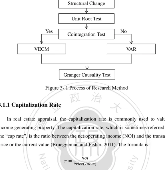
(24) China’s Housing Bubbles and the Driving Factors. Chapter 3 Research Method and Data Information This chapter is divided into two parts. The first part shows the methods for the housing bubbles measurement and the empirical analysis. And the second part describes the variables selected in the empirical analysis.. 3.1 Research Method The purpose of this study is to measure the status of the housing bubbles in the. 政治大. three selected cities and to explore the equilibrium relationship between the housing bubbles and other variables. Based on the literature review，this study defines housing. 立. bubbles as the comparison between fundamental values and market prices. According. ‧ 國. 學. to Lin (2012), the fundamental value of real estate can be calculated by annual rents and reasonable capitalization rate. And the funds which are used to purchase houses usually consist of equity and mortgage. Thus, weighted average cost of capital can be. ‧. regarded as the reasonable capitalization rate which is adopted by most market. y. Nat. participants. In the empirical analysis section, we employ Johansen cointegration. io. sit. method to analyze the housing bubbles of these three cities and other variables. er. respectively. If they have the cointegration relationship, Vector Error Correction. al. n. v i n C h model. Finally, U through Vector Autoregressive (VAR) e n g c h i we use Granger Causality test to find out the lead/lag relationship between the housing bubbles and the variables. In Model (VECM) is applied for further study. Otherwise, they should be interpreted. short, the general process of empirical analysis is as follows:. 17.

(25) China’s Housing Bubbles and the Driving Factors. Structural Change Unit Root Test Yes. No. Cointegration Test. VECM. VAR. Granger Causality Test Figure 3- 1 Process of Research Method. 政治大. 3.1.1 Capitalization Rate. 立. ‧ 國. 學. In real estate appraisal, the capitalization rate is commonly used to value an income generating property. The capitalization rate, which is sometimes referred to as the “cap rate”, is the ratio between the net operating income (NOI) and the transaction. ‧. (3.1). er. io. sit. Nat. 𝑁𝑂𝐼. 𝑟 = 𝑃𝑟𝑖𝑐𝑒(𝑉𝑎𝑙𝑢𝑒). y. price or the current value (Brueggeman and Fisher, 2011). The formula is:. al. n. v i n C h the value of realUestate by determining the NOI the equation above, we can estimate engchi. Generally, NOI is calculated by rental income from operating expenses. According to and dividing by an appropriate 𝑟.. 3.1.2 Weighted Average Cost of Capital In general, the investors use both equity and loan to finance their investments. They must take into account the loan interest they need to pay and the opportunity cost of keeping the money. Accordingly, they expect that their total earnings are more than the costs of capital. To evaluate an investment project, the investors usually discount the future cash flows at the weighted average cost of capital (WACC). The WACC is the minimum return that a project must satisfy its investors (Ross et al., 2009). The formula of WACC works out to be:. 18.

(26) China’s Housing Bubbles and the Driving Factors 𝐸. 𝐷. 𝑅0 = 𝑉 × 𝑟𝐸 + 𝑉 × 𝑟𝑀. (3.2). In this expression, the cost of equity is 𝑟𝐸 and the cost of loan is 𝑟𝑀 ; 𝐸/𝑉 represents the proportion of equity and 𝐷/𝑉 represents the loan-to-value ratio. The income tax base is calculated by NOI from the expenses of interest and depreciation. In other words, interest is tax deductible which can cut the average cost of capital. So the formula of after-tax WACC is as follow： 𝐸. 𝐷. 𝑅0 = 𝑉 × 𝑟𝐸 + 𝑉 × 𝑟𝑀 × (1 − t). (3.3). 政治大. where t is the income tax rate. Since the WACC is the minimum acceptable return, NOI divides by WACC is the reasonable price accepted by most investors.. 立. ‧ 國. 學. 3.1.3 Cointegration Test. In 1987, Engle and Granger proposed the theory of cointegration, which provides. ‧. a new way to build up models for non-stationary series. Although the non-stationary. y. Nat. time series can be rendered stationary through differencing the series, the differencing. sit. series does not have direct economic meanings. However, cointegration which refers. er. io. to linear combinations of non-stationary time series is an alternative method of. al. n. v i n C h implies that there cointegration e n g c h i U exist. achieving stationary. It is noticeable that the series must be integrated of the same order. Furthermore,. long-run equilibrium. relationships between the variables.. Engle and Granger also proposed a testing procedure to confirm whether the non-stationary series are cointegrated. The Engle-Granger test employs the residuals of regression to perform the unit root test. Suppose {yt} and {xt} are I(1), we build up a regression model as follow: 𝑦𝑡 = 𝛽0 + 𝛽1 𝑥𝑡 + 𝑒𝑡. (3.4). In this equation, yt is the dependent variable; xt is the independent variable and et is the error term. Then, we use the {et} sequence which is the estimated residuals from the regression equation above to perform the unit root test. The regression of the 19.

(27) China’s Housing Bubbles and the Driving Factors. residuals can be expressed as: ∆𝑒̂𝑡 = 𝑎1 𝑒̂𝑡−1 + 𝜀𝑡. (3.5). If the estimated result can reject the null hypothesis |𝑎1 | = 0, then we can make a conclusion that the variables are cointegrated. However, the Engle-Granger procedure cannot make the separate estimation of multiple cointegrating vectors. In this two-step method, since the coefficient 𝑎1 is obtained by the residuals of another regression, the errors produced in step1 are carried into step 2. Fortunately, Johansen cointegration test which is proposed in 1991 can avoid the defects above.. 立. 政治大. Johansen cointegration test, which is based on VAR approach, uses the maximum to. ‧ 國. estimation. examine. cointegration. relationships. 學. likelihood. between. the. non-stationary time series. This approach can interpret the multiple long-run equilibrium relationship more robustly. Assuming a VAR model of order p and n. ‧. variables can be expressed as follow:. y. Nat. (3.6). er. io. sit. 𝑦𝑡 = 𝛼1 𝑦𝑡−1 + 𝛼2 𝑦𝑡−2 + ⋯ + 𝛼𝑝 𝑦𝑡−𝑝 + β𝑥𝑡 + 𝜀𝑡. where 𝑦𝑡 is a vector of non-stationary I(1) series; 𝑥𝑡 is a d-vector of exogenous. n. al. Ch. i n U. v. variables; 𝜀𝑡 is disturbance vector. Through subtracting 𝑦𝑡−1 on both sides of the. engchi. equation (3.6), we can obtain a new equation as:. ∆𝑦𝑡 = 𝜋𝑦𝑡−1 + ∑𝑝−1 𝑖=1 𝜋𝑖 ∆𝑦𝑡−𝑖 + β𝑥𝑡 + 𝑢𝑡. (3.7). 𝑝 where π = ∑𝑝𝑖=1 𝛼𝑖 − 𝐼 and π𝑖 = − ∑𝑗=𝑖+1 𝛼𝑗 . In the equation (3.7), we need to pay. attention to the rank of the long-run impact matrix π which equals to the number of cointegrating vectors. Then we can obtain the number of cointegration relationships by examining the non-zero characteristic roots of π. Therefore, Johansen proposed the Trace and Maximum Eigenvalue test to determine the number of cointegration. 𝜆𝑡𝑟𝑎𝑐𝑒 (𝑟) = −𝑇 ∑𝑘𝑖=𝑟+1 ln(1 − 𝜆𝑖 ). 20. (3.8).

(28) China’s Housing Bubbles and the Driving Factors. 𝜆𝑚𝑎𝑥 (𝑟) = −𝑇 ln(1 − 𝜆𝑟+1 ). (3.9). where T is the number of observations and λr is the value of characteristic roots. The null hypothesis of the Trace test is H0: rank≤r. On the other hand, the null hypothesis of the Maximum Eigenvalue test is H0: rank=r.. 3.1.4 Vector Error Correction Model Engle and Granger proposed Vector Error Correction Model (VECM) that is the combination of cointegration and error correction model. VECM provides robust interpretations of both long-run and short-run dynamics. Hence, VECM is an appropriate model for a system of cointegrated variables. The system of cointegrated. 政治大. series can be expressed by VECM as follow:. 立. ‧ 國. 學. ∆𝑦𝑡 = 𝛼𝑒𝑐𝑚𝑡−1 + ∑𝑝−1 𝑖=1 𝜋𝑖 ∆𝑦𝑡−1 + 𝜀𝑡. (3.10). ‧. 𝛼𝑒𝑐𝑚𝑡−1 is the vector of error correction terms, which equals to 𝛽 ′ 𝑦𝑡−1 . It can show the long-run equilibrium relationships between the variables. And the coefficient 𝛼. Nat. sit. y. represents the rate of adjusting deviations. For a more brief explanation, we assume a. io. er. VECM with two series (y1 and y2) which have no lagged differences. Then the set of equations can be written as:. n. al. Ch. ∆𝑦1𝑡 = 𝛼1 (𝑦2𝑡−1 − 𝑏𝑦1𝑡−1. engchi. i n )U+ 𝜀. v. 1𝑡. (3.11a). ∆𝑦2𝑡 = 𝛼2 (𝑦2𝑡−1 − 𝑏𝑦1𝑡−1 ) + 𝜀2𝑡. (3.11b). In the equations, 𝛼1 and 𝛼2 represent the adjustment rate. The variable on the right side of the equations is the error correction term. In the long-run equilibrium relationship, this term should be zero. Hence, once the series (y1 and y2) deviate the equilibrium, the error correction term changes. The coefficients 𝛼1 and 𝛼2 make the deviating series return to the long-run equilibrium.. 3.1.5 Vector Autoregressive Model If there is no cointegration between the time series, Vector Autoregressive (VAR) 21.

(29) China’s Housing Bubbles and the Driving Factors. model is appropriate to explore the dynamic interrelationships between the series. According to the theory of VAR, it requires all the series are stationary. Therefore, the non-stationary series need to be differenced firstly. In the VAR model, every endogenous variable is expressed by the lag values of all the variables. Hence, VAR can predict the relationships between the interrelated series and analysis the impulse of random disturbances on variables. The mathematical expression of VAR can be expressed as: 𝑦𝑡 = 𝛼1 𝑦𝑡−1 + ⋯ + 𝛼𝑝 𝑦𝑡−𝑝 + 𝛽𝑥𝑡 + 𝜀𝑡. (3.12). In this equation, 𝑦𝑡 represents the vector of endogenous variable; 𝑥𝑡 represents the vector of exogenous variable; p is the selected lag order and 𝜀𝑡 is the vector of. 政治大. disturbances. Especially, different 𝜀𝑡 at the same period can be interrelated but would. 立. not related to its own lag value and the variables on the right side of the equation. ‧ 國. 學. (3.12).. ‧. 3.1.6 Granger Causality Test. y. Nat. In the econometric analysis, some variables may be significantly related with no. sit. economic meaning. This is a common problem in the field of econometric. Thus, in. er. io. 1969, Granger proposed the Granger causality test to judge the causal relationship of. al. v i n can be interpreted by the lagged C value U coefficient of x and y is h e nofgx.cIfhthei related significant, we can say that y is caused by x. Based on the theory of Granger causality n. variables. In the Granger causality test, the key to note is that how much the current y. test, if x is the reason of y, x should precede y. The Granger causality equation is defined as: ∆𝑦𝑡 = 𝛼0 + ∑𝑝𝑖=1 𝛼𝑖 ∆𝑥𝑡−𝑖 + ∑𝑝𝑗=1 𝛽𝑗 ∆𝑦𝑡−𝑗 + 𝜀𝑡. (3.13). where 𝑦𝑡 is the dependent variable; 𝑥𝑡 is the independent variable and p is lag terms. The null hypothesis of Granger causality test is H0: 𝛼1 = 𝛼2 = ⋯ = 𝛼𝑝 = 0. If the result of the test accepts the null hypothesis, the variable x cannot cause the variable y which means x is an exogenous variable for y.. 22.

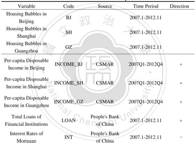
(30) China’s Housing Bubbles and the Driving Factors. 3.2 Data Information 3.2.1 Variable Selection In this study, the selected variables contain total loans of financial institutions, interest rates of mortgage and per-capita disposable income in the three cities. First of all, the real estate industry is capital-intensive. Both the developers and investors are deeply dependent on financing. When the central bank expands the credit scale, the home buyers can get more money from financial institutions easily. Then the demand for houses increases significantly and the housing prices rise accordingly. As long as the easy credit policies continue, the housing bubbles would. 政治大 institutions are positively correlated 立 with the housing bubbles.. constantly accumulate. Thus, this study expects that total loans of financial. ‧ 國. 學. Secondly, interest rate is one of the indispensable macro-control means in China. And in the real estate investment, interest rates of mortgage affect the capital costs. ‧. which cannot be ignored. If interest rates rise, the carrying costs of houses will rise proportionately. Then the speculators change their minds to sell houses at the. y. Nat. sit. appropriate price, instead of hoarding properties. It is likely to reduce housing bubbles.. er. al. n. housing bubbles.. io. Hence, it is considered that the increase of mortgage rates might lead to declines in. Ch. engchi. i n U. v. Lastly, personal income is one of the indicators of economic development. When the economy develops, people's income should increase, which in turn promotes economic development. Furthermore, the domestic economy and real estate industry should also be complementary to each other. Therefore, this study anticipates that personal incomes have a positive relationship with housing bubbles. However, there are obvious income disparities in different cities. Consequently, we select per-capita disposable incomes in Beijing, Shanghai and Guangzhou respectively.. 3.2.2 Data Source The data employed in this study range from January 2007 to November 2012, 71 samples in total. Because the status of housing bubbles is not published data, we 23.

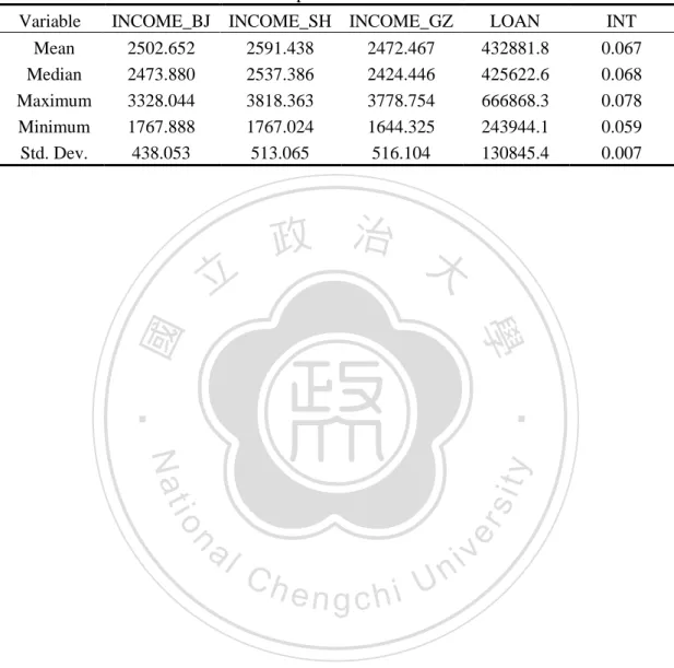
(31) China’s Housing Bubbles and the Driving Factors. would measure it by a specified method in this study. According to the long repayment term of home loan, the lending rate of over 5 years is usually employed as the mortgage rate. The per-capita disposable incomes in the three cities are provided by GTA CSMAR database. Total loans of financial institutions and interest rates of mortgage are reported by People’s Bank of China monthly. However, the original data of disposable incomes is quarterly. Thus, we need to convert the quarterly data into monthly data by Eviews statistical software. Table 3-1 shows the brief information of the variables used in this study. Table 3- 1 The Variable Descriptions Variable Housing Bubbles in Beijing Housing Bubbles in Shanghai Housing Bubbles in Guangzhou. Code BJ. 立SH. Source. Direction. 2007.1-2012.11 政治大 2007.1-2012.11 2007.1-2012.11. 學. GZ. ‧ 國. Time Period. CSMAR. 2007Q1-2012Q4. +. Per-capita Disposable Income in Shanghai. INCOME_SH. CSMAR. 2007Q1-2012Q4. +. CSMAR. 2007Q1-2012Q4. Interest Rates of Mortgage. al. v i n C People's Bank U 2007.1-2012.11 LOAN h e nofgChina chi. n. Total Loans of Financial Institutions. y. sit. INCOME_GZ. er. io. Per-capita Disposable Income in Guangzhou. ‧. INCOME_BJ. Nat. Per-capita Disposable Income in Beijing. INT. People's Bank of China. 2007.1-2012.11. +. + −. 3.2.3 Data Analysis It is helpful for further study to understand the characteristics of the data. The descriptive statistics of variables are shown in Table 3-2, including the mean, median, maximum, minimum and standard deviation. However, the characteristics of the housing bubbles in the three cities will be discussed later because the status of the housing bubbles is going to be calculated in the next chapter. From Table 3-2, INCOME_BJ, INCOME_SH, INCOME_GZ and LOAN have increased a lot during. 24.

(32) China’s Housing Bubbles and the Driving Factors. the research period, which accords with China’s economic growth situation. In addition, since interest rates are controlled by the central bank strictly, interest rates of mortgage do not change much certainly. Table 3- 2 Descriptive Statistics of Variables INCOME_BJ INCOME_SH INCOME_GZ 2502.652 2591.438 2472.467 2473.880 2537.386 2424.446 3328.044 3818.363 3778.754 1767.888 1767.024 1644.325 438.053 513.065 516.104. 立. LOAN 432881.8 425622.6 666868.3 243944.1 130845.4. 政治大. 學 ‧. ‧ 國 io. sit. y. Nat. n. al. er. Variable Mean Median Maximum Minimum Std. Dev.. Ch. engchi. 25. i n U. v. INT 0.067 0.068 0.078 0.059 0.007.

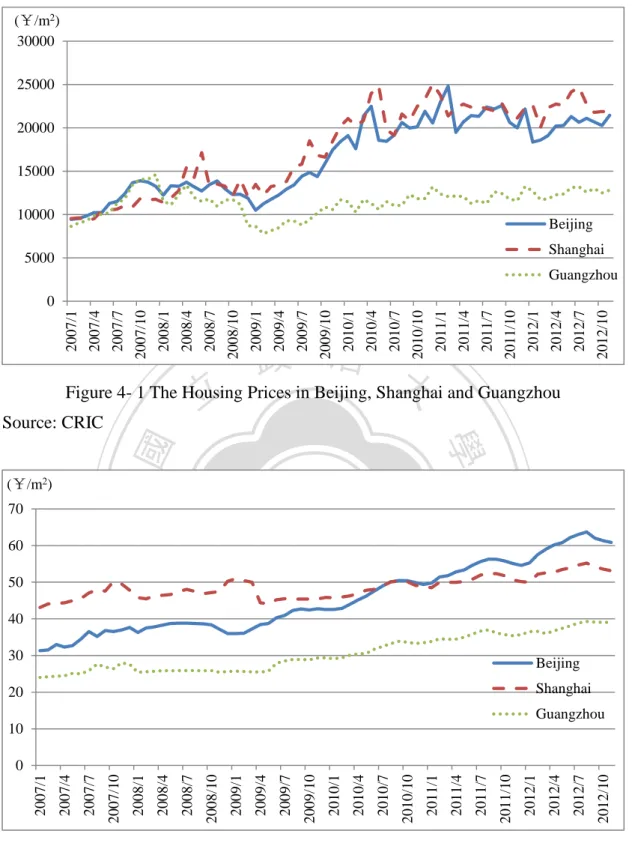
(33) China’s Housing Bubbles and the Driving Factors. Chapter 4 Measure of Housing Bubbles This chapter consists of three parts. The housing prices and rents in Beijing, Shanghai and Guangzhou from 2007 to 2012 are presented in the first part. The second part introduces the parameters used for calculating fundamental values. And the last part describes the situation of housing bubbles in three cities and analyzes the causes of changes.. 4.1 Trends of Housing Prices and Rents. 政治大. The data of housing prices in three selected cities comes from the monthly market. 立. report of China Real Estate Information Corporation (CRIC), as reported in Figure. ‧ 國. 學. 4-1. As we all see, from January 2007 to November 2012, the housing prices had kept increasing in Beijing, Shanghai and Guangzhou. Beijing’s housing price rose from ￥9446/m2 to ￥21447/m2 while the housing price in Shanghai increased from. ‧. ￥9548/m2 to ￥21863/m2. Also Guangzhou’s housing price rose from ￥8622/m2 to. y. Nat. ￥12821/m2. In 2008, China’s real estate market was influenced by the subprime. io. sit. mortgage crisis and the housing prices fell a little bit. However, after several months,. al. n. out of the depression.. er. the housing prices perked up again, which meant that the real estate market had got. Ch. engchi. i n U. v. The housing rents in China’s real estate market are not transparent. So it is quite difficult to obtain the data of housing rents as long as we need. Under this circumstance, we decide to convert the housing rental index into the actual rents. Firstly, we get the housing rents in November 2012 by CityRE Data. Secondly, the trend of the housing rental index is acquired in the China Real Estate Index System. At last, according to the data above, we figure out the housing rents in three selected cities which range from January 2007 to November 2012 (as shown in Figure 4-2). Compared with the housing prices, the rents grew at a slow rate.. 26.

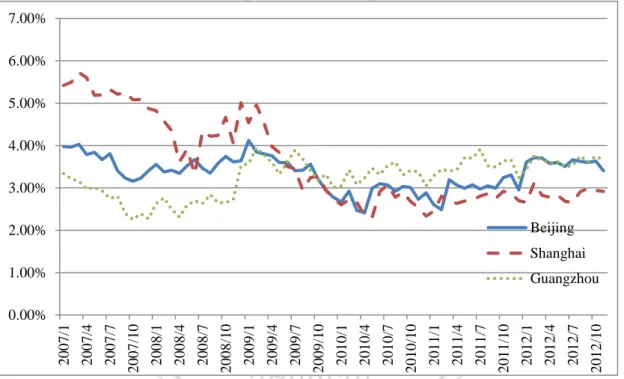
(34) China’s Housing Bubbles and the Driving Factors. (￥/m2) 30000 25000 20000 15000 10000. Beijing Shanghai. 5000. Guangzhou. 70 60. ‧. ‧ 國. 學. (￥/m2). sit. n. al. er. io. 40. y. Nat. 50. 2012/10. 政治大 Figure 4- 1 The Housing Prices in Beijing, Shanghai and Guangzhou 立 Source: CRIC. 2012/7. 2012/4. 2012/1. 2011/10. 2011/7. 2011/4. 2011/1. 2010/10. 2010/7. 2010/4. 2010/1. 2009/10. 2009/7. 2009/4. 2009/1. 2008/10. 2008/7. 2008/4. 2008/1. 2007/10. 2007/7. 2007/4. 2007/1. 0. 30 20. Ch. engchi. i n U. v. Beijing Shanghai Guangzhou. 10. 2012/10. 2012/7. 2012/4. 2012/1. 2011/10. 2011/7. 2011/4. 2011/1. 2010/10. 2010/7. 2010/4. 2010/1. 2009/10. 2009/7. 2009/4. 2009/1. 2008/10. 2008/7. 2008/4. 2008/1. 2007/10. 2007/7. 2007/4. 2007/1. 0. Figure 4- 2 The Housing Rents in Beijing, Shanghai and Guangzhou Source: CityRE and CREIS According to the direct capitalization method, the market capitalization rates in three selected cities are calculated by the housing prices and rents, as reported in Figure 4-3. However, the net operating incomes that we use in this study are the. 27.

(35) China’s Housing Bubbles and the Driving Factors. annual rents and do not take off the operating expenses. In other words, these capitalization rates are higher than the actual values. Even so, in the research period, the capitalization rates are rather low in Beijing, Shanghai and Guangzhou. The capitalization rate in Beijing decreased from 3.98% to 3.40% while the one in Guangzhou increased from 3.34% to 3.66%. They didn’t change much. In contrast, the capitalization rate in Shanghai underwent a big change, which dropped from 5.42% to 2.91%. In light of this, there was a chasm between the housing prices and rents in Beijing, Shanghai and Guangzhou. It implies the housing bubbles might exist in real estate market of these selected cities.. 7.00%. 政治大. 6.00%. 立. 5.00%. y. 2012/10. 2012/7. 2012/4. 2012/1. i n U. Guangzhou. 2011/10. er. v. 2011/1. 2010/10. engchi. 2010/7. 2010/4. 2010/1. 2009/10. 2009/7. Ch. 2009/4. 2009/1. 2008/10. 2008/7. 2008/4. 2007/10. 2007/7. 2007/4. 2007/1. al. n. 2008/1. io. 0.00%. Shanghai. sit. Nat. 1.00%. Beijing. 2011/7. 2.00%. 2011/4. 3.00%. ‧. ‧ 國. 學. 4.00%. Figure 4- 3 The Market Capitalization Rates in Beijing, Shanghai and Guangzhou. 28.

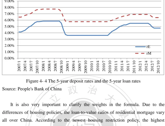
(36) China’s Housing Bubbles and the Driving Factors. 4.2 Fundamental Value In order to obtain the fundamental values, the reasonable capitalization rates should be estimated through the use of the WACC approach first. Based on the formula of WACC, we need to make a decision about the costs of equity and loan. Generally speaking, the interest rate for time deposit is regarded as the cost of equity for property investors. At the moment, time deposits in China offer 6 kinds of investment maturity terms: 3 months, 6 months, 1 year, 2 years, 3 years and 5 years. The owners of houses usually hold the properties for a relatively long period. Therefore, this study chooses the interest rate of the 5-year deposit as the cost of equity. In China, the residential mortgage includes housing fund loan and commercial. 政治大. loan. But the application of housing fund loan is constrained by many regulations and not all citizens have housing fund. The interest rate for commercial loan meets the. 立. actual circs better. The items of commercial loans consist of 6 months, 1 year, 3years,. ‧ 國. 學. 5 years and over 5 years. Since the mortgages usually have long repayment terms, the loan rate of over 5years is employed in home loan2. Although the loan rates are specified by the central bank, the merchant banks could float the rates within a certain. ‧. range. Because the houses are used as the collaterals for the mortgages, the banks. y. Nat. would offer the prime lending rate. This study selects the interest rate of the 5-year. sit. loan as the cost of debt, which is close to the fact. The data of interest rate are shown. n. al. er. io. in Figure 4-4, which is collected from People’s Bank of China.. Ch. engchi. 2. i n U. v. There is no specific mortgage rate in China. In practice, the interest rate of commercial loan is regarded as the mortgage rate directly. 29.

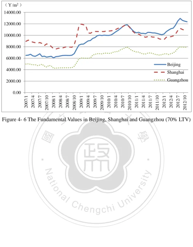
(37) China’s Housing Bubbles and the Driving Factors. 9.00% 8.00% 7.00% 6.00% 5.00% 4.00% 3.00% 2.00%. rE. 1.00%. rM 2012/10. 2012/7. 2012/4. 2012/1. 2011/10. 2011/7. 2011/4. 2011/1. 2010/10. 2010/7. 2010/4. 2010/1. 2009/10. 2009/7. 2009/4. 2009/1. 2008/10. 2008/7. 2008/4. 2008/1. 2007/10. 2007/7. 2007/4. 2007/1. 0.00%. Figure 4- 4 The 5-year deposit rates and the 5-year loan rates. 政治大. Source: People's Bank of China. 立. It is also very important to clarify the weights in the formula. Due to the. ‧ 國. 學. differences of housing policies, the loan-to-value ratios of residential mortgage vary all over China. According to the newest housing restriction policy, the highest. ‧. loan-to-value ratio of the first suite loan is 70% and the highest one of the second suite loan is 50%. For convenience, we calculate the fundamental values in three. Nat. sit. y. chosen cities under the circumstances of 50% and 70% loan-to-value ratio, as reported. io. n. al. er. in Figure 4-5 and Figure 4-6. （￥/m2 ） 16000.00. Ch. 14000.00. engchi. i n U. v. 12000.00 10000.00 8000.00 6000.00 Beijing 4000.00. Shanghai. 2000.00. Guangzhou 2012/10. 2012/7. 2012/4. 2012/1. 2011/10. 2011/7. 2011/4. 2011/1. 2010/10. 2010/7. 2010/4. 2010/1. 2009/10. 2009/7. 2009/4. 2009/1. 2008/10. 2008/7. 2008/4. 2008/1. 2007/10. 2007/7. 2007/4. 2007/1. 0.00. Figure 4- 5 The Fundamental Values in Beijing, Shanghai and Guangzhou (50% LTV). 30.

(38) China’s Housing Bubbles and the Driving Factors. （￥/m2 ） 14000.00 12000.00 10000.00 8000.00 6000.00 Beijing 4000.00. Shanghai Guangzhou. 2000.00. 2012/10. 2012/7. 2012/4. 2012/1. 2011/10. 2011/7. 2011/4. 2011/1. 2010/10. 2010/7. 2010/4. 2010/1. 2009/10. 2009/7. 2009/4. 2009/1. 2008/10. 2008/7. 2008/4. 2008/1. 2007/10. 2007/7. 2007/4. 2007/1. 0.00. 政治大 Figure 4- 6 The Fundamental Values in Beijing, Shanghai and Guangzhou (70% LTV) 立 ‧. ‧ 國. 學. n. er. io. sit. y. Nat. al. Ch. engchi. 31. i n U. v.

(39) China’s Housing Bubbles and the Driving Factors. 4.3 Status of Housing Bubbles As the literature review implies, the definition of housing bubbles can be in a number of ways. From the point of fundamental value, this study defines housing bubbles as the discrepancy between housing fundamental values and market prices. The formula of housing bubbles is as follows: 𝑀𝑃. Bubble = ( 𝐹𝑉 − 1) × 100%. (4.1). In this equation, MP represents the market price of property and FV represents the housing fundamental value. The results are reported in Figure 4-7 and Figure 4-8.. 政治大 make the calculated housing bubbles become bigger than the actuals but do not affect 立 the trends. However, the fundamental values in this study do not consider the tax shield. It would. ‧ 國. 學. 250.00%. ‧. 200.00%. Beijing. sit. n. al. er. io. 100.00%. Guangzhou. y. Nat. 150.00%. Shanghai. Ch. 50.00%. engchi. i n U. v. 2012/10. 2012/7. 2012/4. 2012/1. 2011/10. 2011/7. 2011/4. 2011/1. 2010/10. 2010/7. 2010/4. 2010/1. 2009/10. 2009/7. 2009/4. 2009/1. 2008/10. 2008/7. 2008/4. 2008/1. 2007/10. 2007/7. 2007/4. -50.00%. 2007/1. 0.00%. Figure 4- 7 The Housing Bubbles in Beijing, Shanghai and Guangzhou (50% LTV). 32.

(40) China’s Housing Bubbles and the Driving Factors. 250.00% Beijing Shanghai 200.00%. Guangzhou. 150.00%. 100.00%. 50.00%. 立. 2012/10. 2012/7. 2012/4. 2012/1. 2011/10. 2011/7. 2011/4. 政治大. 2011/1. 2010/10. 2010/7. 2010/4. 2010/1. 2009/10. 2009/7. 2009/4. 2009/1. 2008/10. 2008/7. 2008/4. 2008/1. 2007/10. 2007/7. 2007/4. 2007/1. 0.00%. Figure 4- 8 The Housing Bubbles in Beijing, Shanghai and Guangzhou (70% LTV). ‧ 國. 學. As shown in Figure 4-7, from 2007 to 2009, the housing bubbles in Guangzhou. ‧. were in the first place and the ones in Beijing come second, while the bubbles in Shanghai were smallest. In this period, although the housing prices in Beijing and. Nat. sit. y. Shanghai were higher than the ones in Guangzhou, the housing bubbles in Guangzhou. io. er. were most serious. It might relate to the seriously low housing rents in Guangzhou. In 2008, the subprime mortgage crisis burst out. The housing bubbles in three cities all. n. al. i n U. v. reduced. By early 2009, the housing bubbles in three cities reached their lowest levels. Ch. engchi. and even the ones in Shanghai were negative briefly. After that, the real estate markets in three cities shook off the influence of the subprime mortgage crisis and began to recover gradually. The housing bubbles were going up again. However, in April 2010, a series of house purchase restrictions were announced. At that time, the housing bubbles in Beijing and Shanghai suddenly dropped and then ballooned. When the restrictions were officially implemented, the trends of the bubbles in Beijing and Shanghai merely changed a little. It is thus clear that the house purchase restrictions can curb over-heating property markets in a short time. At the same time, the restrictions also gave confidence to the people who would buy houses to live in. They purchased a large number of properties and made the real estate markets take a good turn. On the other hand, the housing bubbles in Guangzhou edged up after 2009. It is possible that the home buyers in Guangzhou took a wait-and-see attitude towards the 33.

(41) China’s Housing Bubbles and the Driving Factors. real estate market. In Figure 4-8, we can see that the housing bubbles which are calculated under the circumstances of 70% loan-to-value ratio are higher than the ones under the circumstances of 50% loan-to-value ratio. It is more consistent with the practice. From January 2007 to November 2012, there are 21 months in which the housing bubbles in Beijing were more than 100%. And the highest point (135.8%) arose in February 2011. In Shanghai, the housing bubbles exceeded 100% for 27 times and their peak (144.44%) appeared in January 2012. When it comes to Guangzhou, there are 21 months that the housing bubbles were higher than 100%. And the bubbles in Guangzhou peaked at 214.40% in October 2007. Thus it can be seen that the housing. 治政 and Guangzhou. The problem of high housing bubbles 大 cannot be ignored any more. 立. market prices deviated from the fundamental values seriously in Beijing, Shanghai. ‧. ‧ 國. 學. n. er. io. sit. y. Nat. al. Ch. engchi. 34. i n U. v.

(42) China’s Housing Bubbles and the Driving Factors. Chapter 5 Empirical Results This chapter mainly presents the relationship between housing bubbles and the selected variables. First, the existence of structural change and the unit root are checked. Then the results of cointegration test are interpreted. Finally, the results of Granger causality tests provide suggestions for housing polices. Monthly data or quarterly data usually exhibits some form of seasonality (Enders, 1995). The seasonal variation of time series may cover up the actual trends of. 治政 econometric analysis. The variables used in this study, 大 except interest rates, have obvious seasonal patterns. 立 Accordingly, they are seasonally adjusted by using Census. economic processes. So we should deseasonalize the time series before the. ‧ 國. 學. X-12 method3.. ‧. 5.1 Structural Change. y. Nat. Before performing unit root test, it is necessary to confirm that there are no. io. sit. structural changes during the research period. If there are structural breaks, the results. er. of the following econometric analysis would be biased. In order to avoid the deviated. al. n. v i n structural changes or not. In thisCstudy, the Cumulative Sum of the recursive h ewe n gapply chi U. estimation, we would identify whether the time series of housing bubbles has residuals test (CUSUM test).. The results of CUSUM test are shown respectively in Figure 5-1, Figure 5-2 and Figure 5-3. Apparently, from Figure 5-1 to Figure 5-3, the housing bubbles in three cities do not exceed the critical value at the 5% significance level (dashed line). In other words, there are no structural changes in these series of housing bubbles during the research period. Therefore, these time series are appropriate for the following tests, and the results would be authentic.. 3. Census X-12 method is a seasonal adjusted procedure established by Bureau of Census. This procedure is revised for many times and becomes one of the most usual seasonal adjusted methods. Much statistical software can perform the Census X-12 procedure. 35.

(43) China’s Housing Bubbles and the Driving Factors. 30. 20. 10. 0. -10. -20. -30 II. III IV. I. II. 2007. III IV. I. 2008. II. III IV. I. 2009. II. III IV. I. II. 2010. III IV. I. 2011. II. III IV. 2012. 政治大. CUSUM. 立. 5% Significance. Figure 5- 1 Result of CUSUM Test for BJ. 20. ‧. ‧ 國. 學. 30. sit. n. al. er. io. 0. y. Nat. 10. -10. Ch. -20. engchi. i n U. v. -30 II. III IV. 2007. I. II. III IV. 2008. I. II. III IV. 2009. I. II. III IV. 2010. CUSUM. I. II. III IV. 2011. 5% Significance. Figure 5- 2 Result of CUSUM Test for SH. 36. I. II. III IV. 2012.

(44) China’s Housing Bubbles and the Driving Factors. 30. 20. 10. 0. -10. -20. -30 III IV. I. II. 2007. III IV. 2008. I. II. III IV. 2009. II. III IV. I. II. 2010. III IV. 2011. 政治大. CUSUM. 立. I. 5% Significance. Figure 5- 3 Result of CUSUM Test for GZ. ‧. ‧ 國. 學. io. sit. y. Nat. n. al. er. II. Ch. engchi. 37. i n U. v. I. II. III IV. 2012.

(45) China’s Housing Bubbles and the Driving Factors. 5.2 Unit Root Test In the time series data analysis, it is essential to confirm whether the series are stationary or not. With the non-stationary variables, the estimates of the classic regression model might be spurious regression4 results. Thus, we employ Augmented Dickey-Fuller (ADF) test and Phillips-Perron (PP) test to examine all the variables used in this study. The result of unit root tests is reported in Table 5-1. We can learn that housing bubbles in the three cities (BJ, SH and GZ), per-capita disposable incomes in these cities (INCOME_BJ, INCOME_SH and INCOME_GZ), total loans of financial. 政治大. institutions (LOAN), and interest rates of mortgage (INT) accept the null hypothesis at the level order, i.e., these time series are non-stationary. However, they reject the. 立. null hypothesis at the first difference order, becoming stationary series. Hence, all the. ‧ 國. 學. variables used in this study are I(1) series.. ‧. n. al. er. io. sit. y. Nat. BJ SH GZ INCOME_BJ INCOME_SH INCOME_GZ LOAN INT. Table 5- 1 Result of Unit Root Test ADF test PP test Level 1st difference Level 1st difference -2.544 -8.952 *** -2.593 * -8.970 *** -1.796 -9.567 *** -1.813 -9.472 *** -1.080 -7.028 *** -1.546 -7.236 *** 0.966 -6.284 *** 1.707 -6.652 *** 1.546 -4.160 *** 1.719 -11.027 *** 0.189 -9.427 *** 1.646 -11.985 *** 3.043 -6.207 *** 2.228 -6.529 *** -2.086 -2.875 * -1.448 -3.018 **. Ch. engchi. i n U. v. Note: 1. Null hypothesis: The series has a unit root. 2. *, ** and *** denote significance at the 10%, 5% and 1% level respectively.. 4. A spurious regression has high R2 values and high t-ratios yielding results with no economic meaning. 38.