1
行政院國家科學委員會專題研究計畫成果報告
膠結不良沈積岩層之非破壞性探勘與監測(III)
Non-destructive Site Characterization and Performance Monitoring
in Poorly Cemented Sedimentary Rock(3)
計畫編號:
NSC 93-2211-E-009-013-
執行期限:93 年 8 月 1 日至 94 年 7 月 31 日
主持人:林志平 國立交通大學土木工程系
一、中文摘要 膠結不良沈積岩層具有孔隙大、透水性 高、岩體強度遇水容易軟化等特性,構築於 此類地層之地工結構物常因軟岩之弱化而 產生滑動破壞。有鑑於此等地層之取樣不 易,工程性質不容易掌握,本計畫之主要目 的在研究以非破壞性之方法探勘軟弱沈積 岩之力學性質及以電磁波之方法監測地工 結構物於膠結不良沈積岩之表現,並配合其 他子計畫之物理模型及現地承載試驗進行 試 驗 材 料 之 調 查 及 破 壞 機 制 之 監 測 與 研 究。雖然以軟弱層積岩為主題與其他子計畫 整合,但為解決研究期間所發掘之問題,主 要研究成果在於非破壞性探勘與監測之方 法論。其中非破壞性探勘主要針對多頻道表 面波震測法進行研究改良,本年度主要工作 在於探討地層側向變化對於表面波震測之 影 響 , 並 發 展 新 式 的 施 測 方 法 Pseusdo-section Survey。監測方面主要應用 電 磁 波 域 反 射 技 術 ( Time Domain Reflectometry, TDR)研發變形、孔隙水壓、 與含水量等監測技術,本年度以波傳理論為 基礎研究改良監測資料之分析方法,成功推 導考慮傳輸線電阻之波傳模式,可完整模擬 各種監測訊號之波形,並據以改善各式監測 項目資料之分析程序。 本研究計畫為三年期整合型研究計畫 『膠結不良沉積岩層大地工程行為』其中子 計畫之一,本報告簡述本計畫之執行成果。 關鍵詞:軟弱岩盤、時域反射法、表面波譜 法 AbstractPoorly cemented sedimentary rock (soft rock) has high porosity and hydraulic conductivity. Geotechnical failure often occurs in this kind of material as a consequence of the decrease of shear strength upon leaching. Considering the difficulty in obtaining undisturbed samples and determining engineering properties in soft rock, the main objectives of this project are to study non-destructive seismic methods to investigate the mechanical properties of the material and electromagnetic techniques to monitor the performance of geotechnical structures in soft rock. These investigation and monitoring techniques will facilitate laboratory model and field loading tests in other sub projects to study the behavior and failure mechanisms of geotechnical structures in soft rock. To resolve the problems found during this research project, this year’s study focused on improving the methodology of surface wave testing and TDR monitoring. In surface wave testing, the effect of lateral heterogeneity was investigated and a new survey method, called Pseudo-section survey, was proposed. This new survey method in combination with analysis methods proposed in last two years will lead to standardization of surface wave testing. In TDR monitoring, a complete wave propagation model was developed to simulate various geotechnical monitoring scenarios. Methods of data reduction based on the wave propagation model were proposed for various applications. This report briefly describes the study result of this year.
Keywords: Soft Rock, Time Domain
Reflectometry, Spectral Analysis of Surface Wave
2 二、計畫緣由與目的 膠結不良沈積岩之地層甚年輕,砂岩孔 隙大、透水性高,材料性質介乎土壤及岩石 間。由於取樣不易,早期對其力學性質及行 為甚難加以掌握。86 至 88 年間由潘以文教 授擔任總計畫主持人,結合不同專長之研究 人員,共同完成『極軟弱年輕砂、頁岩層之 力學行為』整合型研究計畫。其探討之問題 以軟弱(膠結不良)砂岩的力性質及行為決 定為主,包括:如何取得完整不擾動的試 體?如何獲得足具代表性之岩石性質(包含 自然及岩石之岩相組成,單軸、三軸強度, 剪力強度,應力-應變行為,透水性,依時 行為,砂頁岩界面的力學特性)?其弱化機 制如何?力學行為如何?等。參與之人員研 發出改良式之軟弱岩石取樣與保存技術、適 合 軟 弱 岩 石 使 用 之 高 壓 傍 壓 儀 試 驗 (pressuremeter)儀器、多功能軟弱岩石 孔內試驗裝置、改良式之現地透水試驗方 法、適合軟弱岩石使用之高壓三軸試驗系 統 、 軟 岩 用 微 流 量 控 制 滲 透 儀 、 以 及 suspension P-S Logging 現地波速量測技 術之引進。該研究主要成果為使用這些新開 發或引進的試驗技術,進行了一系列之現地 取樣、試驗與室內之試驗,提出了決定極軟 弱岩石材料力學參數之程序與數值模擬之 方法,成果已在國內外相關之學術期刊、研 討會中發表,『多功能軟弱岩石孔內試驗裝 置』並已獲得中華民國專利(發明第一三零 四五八號)。 軟岩的基本力學性質及其量化之實驗 工具已於前期研究得到相當大之進展,但地 工結構物構築於此類地層之分析與設計,在 國內外相關文獻報導都很有限,仍需進一步 研究,為進一部落實並延續上述學術研究成 果,廖志中及黃安斌教授所主持的『極軟弱 岩石的大地工程行為』整合性研究計劃於 89 年開始執行,由筆者延續前期調查方法 之研究,研發使用時域反射(time domain reflectometry,TDR)與表面波頻譜分析 (spectral analysis of surface wave, SASW)之現地試驗技術來決定軟弱岩石之層 次、力學特性、以及地層位移之監測,其他 子計畫則針對地工結構物中之深基礎、淺基 礎、邊坡、隧道等進行破壞機制之研究,最 終的目標為建議合理可用的調查方法、工程 分析方法與模式(承載力、邊坡穩定、隧道 分析等等)、施工之品管與監測方法等,目 前主要研究成果包括:人造軟岩製作及測 試、基礎模型試驗設備架設、實驗站初步調 查、現地實驗場址規劃、TDR 及表面波頻譜 分析設備建立及測試。本研究群希望再以三 年時間繼續朝最終目標邁進,以詳細、準確 的工址調查,光纖及 TDR 監測系統研發及量 測,結合模型及現地試驗深入探討膠結不良 沈積地層大地工程行為。目前規劃進行之子 計畫除本子計畫外,亦包括膠結不良沈積岩 層的深基礎行為、膠結不良沈積岩層的淺基 礎行為、膠結不良沈積岩坡之行為、膠結不 良沈積岩隧道開挖之物理模型及數值分析 研究、膠結不良沉積岩邊坡受地下水之穩定 影響等。 有鑑於現地試驗的耗時、耗費、困難 性,水對膠結不良沈積岩層工程行為的重要 影響,及工程地球物理與高科技產品(例 如,光纖監測器)於土木工程探勘與監測的 未來必然與需要性,本子計畫之主要研究目 的,在於以非破壞性之方法探勘膠結不良沈 積岩層之力學性質,及以電磁波之方法監測 地工結構物於膠結不良沈積岩之表現,並配 合其他子計畫之物理模型及現地承載試驗 進行試驗材料之調查及破壞機制之監測與 研究。 三、結果與討論 本研究相關之詳細研究成果,列舉於參 考文獻。本年度主要研究成果摘述如下: 非破壞性震波探勘 非破壞性探勘主要針對多頻道表面波 震測法進行研究改良,前期研究首先探討包 括受波器間距所造成之頻率混擾、震測線之 有限長度所造成之頻譜分析洩漏、多重模態 之影響、近場與遠場效應、空間解析度之限 制 等 ( 林 志 平 等 人 , 2002 ; 林 志 平 等 人 , 2003a;Lin and Chang, 2004),並推導出新 的通用性波場轉換法(Lin et al. 2004),可 提高頻散曲線分析的解析度與正確地資料 取 樣 以 利 反 算 分 析 ( Lin and Chang, in preparation),本年度主要工作在於探討地 層側向變化對於表面波震測之影響,並發展 新式的施測方法 Pseusdo-section Survey (林 俊宏 2005;Lin and Lin, in preparation)。本 研究採用四級速度-應力有限差分法及錯置
3 網格(staggered grid)模擬表面波在地層具 側向變化情況下之波傳特性,如圖一所示, 當地層具側向變化時,表面波在空間上不在 是 stationary signal 。 圖 二 顯 示 此 non-stationary property 會造成頻散分析的假 頻散現象,而使得表面波反算產生錯誤的地 層波速剖面。 雖然目前有許多 non-stationary 的訊號 分析方法,如小波轉換,但前期研究顯示頻 散分析所能得到之最大波長(即探測深度) 取決於測線展距,non-stationary 的訊號分 析 方 法 可 能 可 以 解 決 波 長 的 側 向 變 化 問 題,但將影響頻散分析所能得到之波長範 圍。因此本研究,持續發展前期所提出之 Pseudo-section 施 測 方 法 ( 圖 三 ) , 配 合 seaming 的相位處理技術處理 pseudo-section 施測法所產生之靜態誤差(圖四),可有效 縮短實際施測展距而不影響頻散分析所需 之展距,且可降低側向變化之影響。綜合上 述成果及前期所提之表面波頻散分析方法 將於近期正式提出表面波震測之標準化程 序(林志平等人 2004a;林志平等人 2005; Lin et al. 2005a)。
圖一 側向地質變化對於表面波之影響 圖二 地層側向變化造成假頻散現象 圖三 Pseudo-section 施測法 圖四 Seaming 相位處理技術消除靜態誤差 電磁波監測 膠結不良沈積岩層之重要監測項目包 括變形、孔隙水壓、含水量等,傳統電子主 動式監測技術之耐久性與可靠度不佳,本研 究強調被動式電磁波監測技術之開發。電磁 波監測主要利用導波管(Wave guide)之設 計及時域反射(TDR)之原理,使其可感應錯 動變形、伸縮變形、孔隙水壓、及含水量等。 TDR 所 發 送 之 電 磁 波 為 引 導 波 (Guided Wave),以同軸電纜將電磁波引導至需要監 測之地點。利用不同機制,時域反射法可用 於監測地層錯動、變位、孔隙水壓等物理 量。前期研究已開發新式導波感測器(林志 平等人 2003b;Lin and Tang, 2005;Lin et al., accepted;Lin et al., revised),並獲得兩項專 利(林志平、湯士弘 2004;林志平等人 2004b),使得 TDR 監測系統具備多種地層 監測功能,可使用同一電子儀器及多工器同 時進行多點,多功能之監測。 本年度持續以波傳理論為基礎研究改 良監測資料之分析方法,成功推導考慮傳輸 線電阻之波傳模式(圖五),可完整模擬各 種監測訊號之波形,並據以改善各式監測項 目資料之分析程序(Lin et al. 2005b;湯士 弘等人 2005;Lin and Tang, submitted;Tang and Lin, in preparation)。其中變形監測之量 化分析最具挑戰性,以波傳模式模擬埋設纜 線受直剪之反射訊號(如圖六),進行參數
4 研究,配合現地安裝方法,提出可行的量化 分析方法,將於近期提出專利申請(Tang and Lin, in preparation)。 圖五 TDR 監測系統之傳輸線波傳模型 圖六 TDR 變形監測量化分析 四、參考文獻
Lin, C.-P., Chang, T.-S. (2004), "Multi-station analysis of surface wave dispersion," Soil Dynamics and
Earthquake Engineering, Vol 24/11, pp. 877-886.
Lin, C.-P., Chang, C.-C., and Chang, T.-S. (2004), "The Use of MASW Method in the Assessment of Soil Liquefaction Potential," Soil Dynamics and
Earthquake Engineering, Vol 24/9-10, pp 689-698. Lin, C.-P. and Tang, S.-H. (2005), " Development and
calibration of a TDR extensometer for geotechnical monitoring," Geotechnical Testing Journal, Vol. 28, No. 5, Paper ID: GTJ12188.
Lin, C.-P., Chang, T.-S., and Lin, C.-H. (2005a), “Towards the Standardization of Multi-station Surface Wave Method for Site Investigation,” Symposium on the Application of Geophysics to Engineering and Environmental Problems, 18th Annual Meeting SAGEEP 2005, Atlanta, USA, pp. 199-214. Lin, C.-P., Chung, C.-C, Tang, S.-H.. (2005b),
“Frequency Domain Analyses of TDR Waveforms for Soil Moisture Measurements,” Symposium on the Application of Geophysics to Engineering and Environmental Problems, 18th Annual Meeting SAGEEP 2005, Atlanta, USA, pp. 1061-1074. Lin, C-P, Chung, C.-C., and Tang, S.-H., "Development
of TDR Penetrometer through Laboratory
Investigations: 1. Measurement of Soil Dielectric Constant" Geotechnical Testing Journal (Accepted). Lin, C-P, Chung, C.-C., and Tang, S.-H., "Development
of TDR Penetrometer through Laboratory Investigations: 2. Measurement of Soil Electrical Conductivity" Geotechnical Testing Journal, (Revised).
Lin, C.-P. and Tang, S.-H., “Accurate Wave
Propagation Model to Improve TDR Interpretations for Geotechnical Applications,” Journal of
Geotechnical and Geoenvironmental Engineering, (submitted).
Lin, C.-P. and Lin, C.-H., “Effect of Lateral
Heterogeneity on Surface Wave Testing: Numerical Simulation and Countermeasure,” Journal of Environmental and Engineering Geophysics, (In preparation).
Tang, S.-H. and Lin, C.-P., “Quantification of Cable Deformation with Time Domain Reflectometry: Implication to Slope Monitoring,” Journal of
Geotechnical and Geoenvironmental Engineering, (in preparation)
Lin, C.-P and Chang, T.-S., “Resolution and Data Sampling of Wavefield Transformation for Surface Wave Analysis,” Journal of Environmental and Engineering Geophysics, (in preparation).
林志平、張正宙、鄭孟雄(2002),"以多頻道表面 波量測地層之剪力波速",2002 岩盤工程研討會論 文集,民國 91 年。 林志平、張宗盛、林智勇、鄭孟雄(2003a),"多頻 道表面波頻散分析",中華民國第十屆大地工程學 術研討會,中華民國 92 年。 林志平、湯士弘、葉志翔、楊培熙、盧吉勇(2003b), "TDR 山坡地監測系統之研發",中華民國第十屆大 地工程學術研討會,中華民國 92 年。 林志平、湯士弘(2004),「時域反射伸縮計」,中華 民國專利證書,發明第 202709 號,專利權期間自 中華民國 93 年 5 月 11 日至 112 年 5 月 14 日止。 林志平、張宗盛、陳逸龍(2004a),”Towards the
standardization of Multi-station Surface Wave Method for Site Investigation,” 第十二屆非破壞性 檢測技術研討會,中華民國非破壞性檢測協會年度 會議,p. 213-221,中華民國 93 年。 林志平、周家榮、湯士弘(2004b),「時域反射圓錐 貫入器」,中華民國專利證書,發明第 202710 號, 專利權期間自中華民國 93 年 5 月 11 日至 112 年 5 月 14 日止。 林志平,張宗盛,林俊宏(2005),"多頻道表面波 試驗標準化之研究",中華民國第十一屆大地工程 學術研討會。 湯士弘,林志平,鐘志忠(2005),"時域反射技術 應用於邊坡監測—成效與問題",中華民國第十一 屆大地工程學術研討會。 林俊宏(2005),”Pseudo-section 概念於表面波震測 應用之研究”,國立交通大學碩士論文。
表 Y04
行政院國家科學委員會補助國內專家學者出席國際學術會議報告
93 年 10 月 13 日 報告人姓名 林志平 服務機構及職稱 國立交通大學,副教授 時間 會議 地點 9/19/2004 ~ 9/22/2004 葡萄牙,Porto 本會核定 補助文號 NSC 93-2211-E-009-013 預核 會議 名稱 (中文)第二屆國際工址調查研討會 (英文)2ndInternational Conference on Site Characterization
發表 論文 題目
(中文)軟研隧道崩塌後之工址調查 TDR 介電貫入器之研發
(英文)Site Characterization for the Investigation of Tunnel 8 Collapse Development of a TDR Dielectric Penetrometer
報告內容應包括下列各項: (見下頁) 一、參加會議經過
第二屆國際工址調查研討會於 2003 年 9 月 19~22 日,在葡萄牙波多市召開。該項會議 由國際土壤力學及大地工程學會(ISSMGE)TC16 策劃。研討會論文集共收錄近 200 篇 論文,與會人士約 500 人。本人與研究同僚共發表兩篇論文「Site Characterization for the Investigation of Tunnel 8 Collapse」、「Site Characterization for the Investigation of Tunnel 8 Collapse」。黃安斌教授還受邀發表 Keynote Lecture 「Advanced Calibration Chambers for Cone Penetration Testing in Cohesionless Soils」。參與團對並積極爭取在台灣主辦下一屆 之國際工址調查研討會,並獲得支持。
二、與會心得
每個 Session 一開始為 Keynote Lecture,共有 11 場精彩的 Keynote Lecture,此外由 Pfof. Hai-Sui Yu 發表 J.K.Mitchell Lecture。由於擔任報告的學者專家對於地工調 查皆有多年的專研,因此大部分場次都十分精彩。本次研討會除傳統地工調查方法,這 次會議的特色是包含許多地球物理方法相關論文的發表,顯現傳統現地試驗與工程地物 探測的結合,是一項重要的趨勢。除了聆聽這些內容充實的專題演講外,又可與諸多學 家面對面交換意見,可說是受益良多、不虛此行。 三、建議 本次爭取在台灣主辦下一屆的會議,已獲得 TC16 的支持。國內有許多相關研究成果, 未來應該多組成團隊參與國際學術交流,以發揮較大的影響力,並爭取在國內舉辦國際 學術研討會,提升國內研究水準。 四、攜回資料名稱及內容 論文集(Vol.1 and Vol.2)
Development of a TDR Dielectric Penetrometer
C.-P. Lin, C.-C. Chung & S.-H. Tang
Dept. of Civil Engineering, National Chiao Tung University, Hsinchu, Taiwan
Keywords: dielectric permittivity, conductivity, time domain reflectometry (TDR), CPT
ABSTRACT: Electrical properties of a soil include the electrical conductivity and dielectric permittivity. Conventional electrical probes measure only the resistivity (the reciprocal of the electric conductivity) of the soil. Interpretation of the resistivity alone for soil physical properties is difficult because it is sensitive to many factors, such as water content, soil types and ground water characteristics. The Time Domain Reflec-tometry (TDR) is a geophysical test method based on electromagnetic waves. It can be used to make simulta-neous measurements of electrical conductivity, apparent dielectric constant, and dielectric constant at differ-ent frequencies of a soil. The dielectric properties provide extra information related to soil physical properties. Current TDR probes can only apply to soils at surface. The paper describes the development of a TDR cone penetrometer that is capable of providing continuous TDR measurements during the cone penetra-tion. Various probe configurations were experimentally studied. The data reduction method for the determi-nation of apparent dielectric constant and electrical conductivity has been formulated and calibrated. The re-gion of influence around the probe and the effect of penetration on TDR measurements are also studied.
1 INTRODUCTION
Conventional in situ testing methods, such as SPT, CPT, and DMT, focus on mechanical response of the soil under test. The physical properties of a soil, such as water content, void ratio, and physical chem-istry of pore water, are of greater concern in geo-environmental concerns. Soil-water interaction and soil microstructure are also important to the renewed focus on the fundamentals of soil behavior.
Physical properties of soils are estimated using laboratory techniques on samples retrieved from a borehole or test pit. While measurements can be made in the field, in general, these measurements are made after the field investigation and on a limited number of samples. Hence, questions arise as to how representative laboratory samples are of the ac-tual field conditions. In particular, it is relatively difficult to obtain undisturbed sample in a sand de-posit. It is also costly and time consuming to obtain physical properties using traditional drilling and laboratory techniques.
Field tests for characterizing soil physical proper-ties are likely to be implemented using electrical methods. Electrical properties of a soil include the electrical conductivity and dielectric permittivity. Most electrical probes measure only the resistivity
(the reciprocal of the electric conductivity) of the soil. Interpretation of the resistivity alone for soil physical properties is difficult because it is sensitive to many factors, such as water content, soil types and ground water characteristics. The Time Domain Reflectometry (TDR) is a geophysical test method based on electromagnetic waves. It can be used to make simultaneous measurement of electrical con-ductivity, apparent dielectric constant, and dielectric constant at different frequencies of a soil. The di-electric properties provide extra information related to soil physical properties.
Current TDR probes can only apply to soils near ground surface. A research to develop an efficient field method to estimate various physical properties of soils using time domain reflectometry was under-taken by the National Chiao Tung University in Taiwan. An initial objective of the research project was to better utilize the electrical properties for characterizing microscopic properties of soils. The main steps of the research are:
1. development of field probes suitable for TDR measurements of soils at various depths,
2. construction of homogenization models for soil electrical properties as a function of soil compo-sition.
3. development of dielectric spectroscopy of soils using the field probe, and
4. development of theoretical or semi-empirical re-lations to extract soil physical properties from electrical properties.
As part of phase one, a TDR probe was developed to be used in conjunction with the Cone Penetration Test or deployed as a permanent sensor with the CPT. The probe was specifically designed to be di-rectly inserted into soil without the need for digging, drilling, or other types of soil preparation. This pa-per describes details of the probe design and meas-urements that can be done.
2 BACKGROUND AND THEORY 2.1 Time Domain Reflectometry
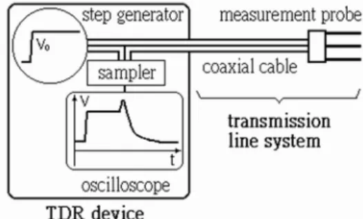
The basic principle of time domain reflectometry (TDR) is the same as radar. But instead of transmit-ting a 3-D wave front, the electromagnetic wave in a TDR system is confined in a waveguide. Figure 1
shows a typical TDR measurement setup composed of a TDR device and a transmission line system. A TDR device generally consists of a pulse generator, a sampler, and an oscilloscope; the transmission line system consists of a leading coaxial cable and a measurement waveguide. The pulse generator sends an electromagnetic pulse along a transmission line and the oscilloscope is used to observe the returning reflections from the measurement waveguide due to impedance mismatches. Such instruments have been used since 1930's for cable testing prior to Fellner-Feldegg (1969) using them for measuring dielectric properties of liquids. The concept has been ex-tended to measurements of electrical properties of soils in which TDR probes are embedded (Topp et al. 1980; Dalton et al. 1984; Heimovaara 1994; Lin 2003).
2.2 Measurements of electromagnetic properties The electrical properties of a soil include dielec-tric permittivity (ε) and electrical conductivity (σ). The dielectric permittivity is in general a complex number and a function of frequency. The equivalent dielectric permittivity (ε*), representing the total ef-fect of the frequency-dependent complex dielectric permittivity (ε) and the conductivity (σ) of a soil, can be written as, (Ramo et al., 1994)
⎟⎟ ⎠ ⎞ ⎜⎜ ⎝ ⎛ + − = + = 0 2 ) ( " ) ( ' ) ( ) ( ' ) ( * ε π σ ε ε ε ε ε f f j f f j f f ii (1)
where f is the frequency; j is (-1)1/2; ε’ and ε” are the real and imaginary parts of dielectric permittivity, respectively; εii is the imaginary part of the
equiva-lent dielectric permittivity, and ε0 is the dielectric permittivity of free space.
Figure 1. A typical configuration of a TDR measurement sys-tem.
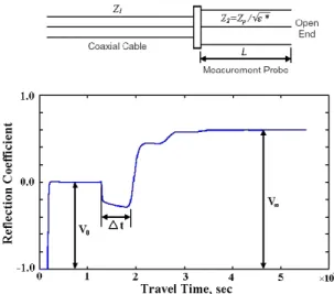
The transmission line wave equation derived from Maxwell's equations governs the electromagnetic wave propagation in a transmission line. Propaga-tion constant and characteristic impedance are two intrinsic parameters that can be defined in the gen-eral solution of the wave equation. The propagation constant, a function of the dielectric permittivity of the insulating material between conductors, deter-mines the phase velocity and attenuation of the wave propagation. The characteristic impedance is a func-tion of the cross-secfunc-tional geometry of the conduc-tors as well as the dielectric permittivity of the insu-lating material between the conductors. Some electromagnetic wave is reflected and recorded by the TDR device if the impedance changes along the transmission line.
Since the dielectric permittivity of the insulating material depends on frequency, the propagation ve-locity is also a function of frequency. The TDR waveform recorded by the sampling oscilloscope is a result of multiple reflections and dispersion. A typi-cal TDR output waveform is shown in Fig. 2. The experimental time-domain information may be treated in the frequency domain to obtain the dielec-tric permittivity as a function of frequency (Giese & Tiemann 1975; Heimovaara 1994; Lin 2003). This involves deriving the system function as a function of the impedance, propagation constant, and bound-ary conditions and it has different form depending on the configuration of the probe. The system func-tion for the field probe to be developed involves much work in electromagnetics and is the main scope of phase three of the multiphase research pro-ject. However, simple methods are available for de-termining apparent dielectric constant and electrical conductivity.
The propagation velocity (v) of an electromag-netic wave that travels in a material with equivalent dielectric permittivity (ε*) is a function of frequency since the dielectric permittivity depends on fre-quency. It can be written as, (Ramo et al., 1994)
⎟⎟ ⎟ ⎠ ⎞ ⎜⎜ ⎜ ⎝ ⎛ ⎟⎟ ⎠ ⎞ ⎜⎜ ⎝ ⎛ + + = 2 ) ( ' ) ( 1 1 2 ) ( ' ) ( f f f c f v ii ε ε ε (2)
where c is the speed of light. The denominator in Eq 2 can be considered as the apparent dielectric per-mittivity of each frequency component. Topp et al. (1980) ignored the dielectric relaxation and loss and assumed the denominator to be a constant. Accord-ingly, the denominator in Eq 2 was replaced by the apparent dielectric constant (Ka) and the correspond-ing propagation velocity was called apparent veloc-ity (va). Ka can be determined from the measured va to be, L t c v c K a a 2 ∆ = = (3)
va is determined from the time difference between
the arrivals of the two reflections (as shown in Fig. 2) and the round-trip length of the probe in the soil.
Figure 2. Interpretation of the TDR waveform to estimate ap-parent dielectric constant and electrical conductivity.
The electrical conductivity (σ) can be measured using the zero-frequency response, which is readily obtained from the reflected signal at long time, once all multiple reflections have taken place and equilib-rium is reached (i.e. V∞ in Fig. 2). According to the derivation of Giese & Tiemann (1975), the electrical conductivity can be written as
∞ ∞ + = ⎟⎟ ⎠ ⎞ ⎜⎜ ⎝ ⎛ − ⎟⎟ ⎠ ⎞ ⎜⎜ ⎝ ⎛ ⎟ ⎠ ⎞ ⎜ ⎝ ⎛ = V c c V V Z Z L c s p 2 1 0 0 1 2 ε σ (4)
where L is the length of the probe, Zp is the imped-ance of the probe filled with air, Zs is the output im-pedance of the TDR device (typically 50 ohm), V0 is the amplitude of the signal coming from the TDR system, and V∞ is the asymptotic value of the re-flected signal. For probes of known characteristics, Zp may be calculated from probe dimensions (Ramo
et al., 1994). Alternatively, the lumped parameters (or called probe constants) c1 and c2 can be inferred from TDR measurements in media of known electri-cal conductivities.
3 PROBE DESIGN AND CALIBRATION 3.1 Probe design
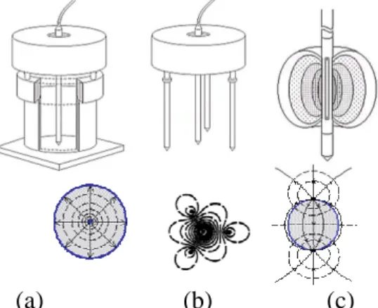
Waveguides or probes for TDR measurements are primarily of two types: coaxial type and multi-conductor type, as shown in Fig. 3(a) and 3(b). The coaxial type of probe is composed of a cylindrical cylinder (CC) acting as the outer conductor and a rod along the centerline of the cylinder acting as a central conductor. The multi-conductor type of probe is composed of one or more rods acting as the outer conductors and a center rod as the inner con-ductor. The coaxial type of probe is adopted for laboratory measurements such as in the compaction mold or in a Shelby tube, using the cylindrical cyl-inder as the outer conductor with the inner conductor being a rod inserted along the centerline of the soil in the mold. The multi-conductor probes can be used for in-place measurements. Conventional multi-conductor probes are 30 cm long and therefore difficult to insert at depths below a few feet. In or-der to adapt the TDR technique to a cone penetrome-ter application a new design is required for the probe. The multiple conductors are placed around a non-conducting shaft to form a TDR probe as shown in
Fig 3(c).
Also shown in Fig. 3 are the electrical potential distributions corresponding to the cross-sections of different probe types. The electrical field is con-tained in the CC for a coaxial probe while it is open in multi-conductor probe. The material near the cen-ter conductor contributes more to the TDR response, and hence has higher spatial weighting to the dielec-tric properties measured from the TDR response.
Baker & Lascano (1989) and Knight (1992) have studied the spatial sensitivity of the measured dielec-tric permittivity. It should be noted that the material inside the shaft of the TDR cone penetrometer is dif-ferent from the surrounding material to be measured by design. Therefore, calibration procedures need to be developed for measurements of the apparent di-electric constant and di-electrical conductivity. In ad-dition, probe should be designed to minimize the ef-fect of the material inside the shaft and maximize the influence zone in the surrounding medium. A series of prototype probes were constructed in the lab to obtain the optimal configuration for the waveguide. The variables considered include the number of con-ductors and conductor width (or spacing). The PVC tubes were used as the shaft and copper strips as the waveguide conductors. The configurations of the prototypes were summarized in Table 1.
(a) (b) (c)
Figure 3. Configurations of types of transmission lines and il-lustrations of their associated electrical potential distribution. TABLE 1. Probe types with different conductor configurations.
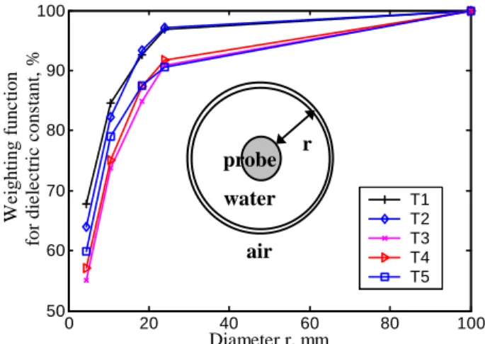
Type No. Copper width (mm) Copper length (mm) No. of copper Probe type T1 20 200 4 T2 30 146 3 T3 20 200 2 T4 10 200 2 T5 3 200 2
3.2 Calibration for dielectric constant and electrical conductivity
The dielectric constant measured by the penetrome-ter probe is a weighted average dielectric constant of the soil and the probe material between the conduc-tors. A convenient homogenization model is based on Birchak's exponential model (Birchak et al. 1974), in which the effective (or measured) apparent dielec-tric constant (Ka,eff) is related to the soil dielecdielec-tric constant (Ka,soil) and probe dielectric constant
(Ka,probe) as
(
)
(
)
(
)
n probe a n soil a n eff a a K a K K , = , +(1− ) , (5)in which n is an empirical constant that summarizes the geometry of the medium with respect to the ap-plied electric field and a is a weighting factor of the surrounding soil. According to Birchak et al. (1974), the theoretical value for n is 1.0. The last term in Eq 5 can be lumped as an empirical parameter b, since the probe dielectric constant is a constant. The soil
dielectric constant can be determined from the TDR penetrometer measurement as
(
)
(
)
a b L t c a b K K n n eff a n soil a − ⎟ ⎠ ⎞ ⎜ ⎝ ⎛ ∆ = − = 2 , , 2 (6) where n, a and b are calibration parameters fordi-electric constant.
Similarly, the probe material between the conduc-tors affects the effective electrical conductivity. Fol-lowing the same reasoning for dielectric constant and assuming n =1, the soil electrical conductivity can be determined from the TDR penetrometer measurement as ∞ + = V β α σ (7)
where α and β are calibration constants for electrical conductivity.
4 EVALUATION OF PROBE PEFORMANCE The multi-conductor penetrometer waveguides may have different features in the TDR response depend-ing on the number of conductors and conductor width. The optimum probe configuration should re-sult in TDR waveforms in which travel time analysis can be easily performed. In addition, the effective dielectric constant should be as close to the soil di-electric constant as possible, and the probe have an influence zone around it as far as possible. These features associated with various probe types listed in Table 1 were evaluated.
4.1 TDR waveforms and effective dielectric
constant
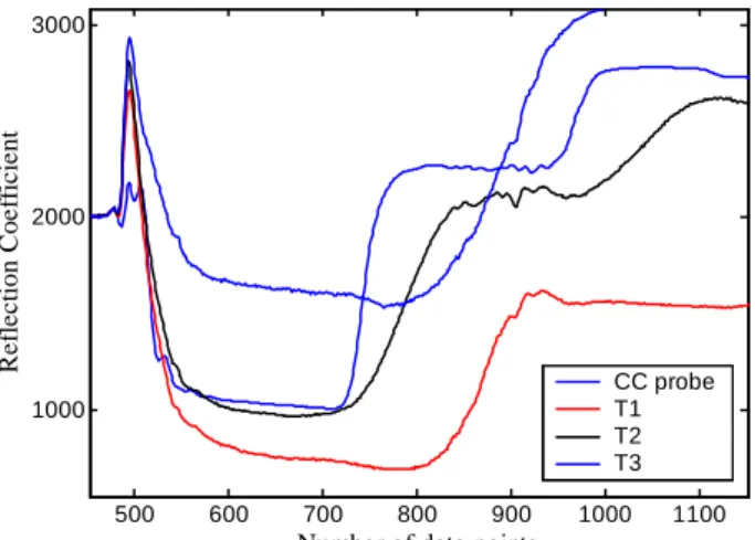
Time domain reflectometry measurements were made by attaching the TDR probe to a Tektronix 1502C (Tektronix, Beaverton, Or) via 2 m of 50-ohm coaxial cable fitted with 50-50-ohm BNC connec-tors at each end. The multi-conductor penetrometer waveguides were submerged in a big tank filled with tap water. Figure 4 shows the TDR waveforms in water for waveguides with different number of con-ductors. Similarly, the waveforms in water for 2-conductor waveguides with different 2-conductor width are shown in Fig. 5. The waveform of a coax-ial probe is also shown in Fig. 4 and Fig. 5 for com-parison. The length of the coaxial probe is 116 mm. The length of the penetrometer waveguide is 200 mm except for probe T2. The TDR sends a step pulse down the cable and some of the wave energy is reflected from both the beginning and end of the probe as shown in Fig. 4 and Fig. 5. The first posi-tive reflection is due to the connector between the cable and the probe. The sudden drop of the
wave-form resulting from the negative reflection occurs when the pulse enters the probe section. And the second positive reflection occurs at the end of the probe. As the number of conductors and conductor width increases, the impedance of the probe de-creases and the negative reflection at the beginning of the probe increases, causing the waveform drops down to a lower level. In terms of waveform shape, the reflections in probe T1 is more apparent and can be easily identified. 500 600 700 800 900 1000 1100 1000 2000 3000 Ref lect io n Co ef fi ci en t
Number of data points
CC probe T1 T2 T3
Figure 4. The TDR waveforms of probes with different number of conductors. 400 500 600 700 800 900 1000 1100 1000 2000 3000 Ref lec ti o n C o ef fi ci en t
Number of data points
CC probe T3 T4 T5
Figure 5. The TDR waveforms of probes with different con-ductor spacing (width).
Waveforms of the penetrometer probes are more dispersive (i.e. rise time of the step pulse is longer) than that of the coaxial probe. This is due to the connector between the BNC connector and the pro-totype probes. The traveltime ∆t of the penetrometer probe is about 75% of that of the coaxial probe of the same length. All penetrometer probes perform similarly in this regard. The effective dielectric con-stants measured by the probes listed in Table 1 are all near 42, which is approximately equal to
(Ka,water+Ka,probe)/2, in which Ka,water = 80 and Ka,probe
≈ 4. Considering the theoretical value n=1.0, Eq 5 can be simplified as 2 , , , probe a soil a eff a K K K = + (8)
for TDR dielectric penetrometers shown in Table1.
4.2 Radial sampling in TDR measurements
The radial sampling in TDR measurements may be investigated using electromagnetic field theory. Al-ternatively, an experimental approach was taken since the theoretical derivation is too complicated and need to be experimentally verified. In order to investigate the radial sampling in TDR measure-ments using the dielectric penetrometers, the proto-type probes were submerged in water-filled PVC tubes of different diameters. Since the dielectric constant of water and air are in two opposite extreme,
Ka,wate =80 and Ka,air = 1.0. The spatial weighting
function may be defined experimentally as % 100 ) ( , , × = eff a r a K K r F (9)
where Ka,r is the effective dielectric constant meas-ured in an water-filled PVC tube with inner diameter
r and Ka,eff is the effective dielectric constant
meas-ured in a big water-filled tank.
For different probe configurations, the spatial weighting function (F) can be plotted as shown in
Fig. 6. The effective dielectric constant becomes asymptotic at a distance of 100 mm and greater. The majority of the electromagnetic response occurs within the first several centimeters in the radial di-rection. The spatial bias for the two-conductor probes (T3, T4, and T5) is slightly less than the three-conductor probe (T2) and four-conductor probe (T1); while Probe T1 and T2 have similar spa-tial weighting function. For the two-conductor figuration, the spatial bias is independent of the con-ductor width. Similarly, the weighting function for electrical conductivity is shown in Fig. 7. The mate-rial near the probe weights even more in conductiv-ity than dielectric constant.
While probes T1 and T2 are more sensitive to near material in terms of dielectric constant; they are less sensitive in conductivity relative to 2-conductor probes (T3, T4, and T5). Observations from Fig. 6
and Fig. 7 raise the concern for the penetration (dis-turbance) effect on Ka and σ measurements in soils. The soil displaced by the penetrometer is likely to change the density of soil adjacent to the penetrome-ter. The nature of variation in density around the penetrometer due to cone penetration will influence the dielectric constant and electrical conductivity. This should be a common problem to all electrical probes that has been overlooked in the past.
0 20 40 60 80 100 50 60 70 80 90 100 W e ig htin g f u nc tion fo r d iel ect ri c co n st a n t, % Diameter r, mm T1 T2 T3 T4 T5
Figure 6. Spatial weighting function for dielectric constant.
0 20 40 60 80 100 50 60 70 80 90 100 W e ight in g f unct ion fo r conduct ivt iy , % Diameter r, mm T1 T2 T3 T4 T5
Figure 7. Spatial weighting function for electrical conductivity.
5 SIMULATED PENETRATION TEST
A TDR dielectric penetrometer was actually fabri-cated using the design similar to type T1. Type 1 may not be the optimum configuration as shown in
Fig. 6. However it was selected at the time when the major concern was to have TDR reflection that can be identified most easily for all cases (i.e. from dry to wet soils). Figure 8 illustrates the design and pic-ture of the probe. The probe consists of four arc-shape stainless steel plates and a delrin shaft. The thickness of the stainless steel was maximized to in-crease the axial strength of the probe. The stainless steel plates were fit into four grooves in the delrin shaft and fastened with screws. This probe was used to perform simulated penetration test in a calibration chamber.
5.1 Results of calibration
The TDR penetrometer shown in Fig. 8 differs from Type 1 probe in that thick conductors are embedded in a dielectric shaft instead of thin conductors bonded to the surface of the dielectric shaft. Cali-bration tests need to be carried out before it can be put into used for measurements of dielectric constant and electrical conductivity. Several liquids of
known dielectric constants and electrical conductivi-ties were used for calibrating the probe using Eqs 6 and 7. The materials used for calibrating dielectric constant were air, butanol, ethanol, and water; while water with different amount of added NaCl was used for calibrating electrical conductivity. Assuming theoretical value n =1.0, the calibrated parameters a = 0.34 and b = 1.91, respectively. If n remained un-known during calibration, the calibrated parameters a = 0.35, b = 1.78, and n = 0.96. Note that the a value is smaller than 0.5, as suggested by Eq 8, be-cause the thick conductor plates are embedded in the delrin grooves instead of stick to the surface. Using the calibrated parameters, the apparent dielectric constants of the calibrating liquids are plotted against their known values in Fig. 8. Both calibrated results provide fairly good fit. The theoretical value
n = 1.0 is also verified in Fig. 9. For simplicity, n
=1.0, a=0.34, and b=1.91 are used. Similarly, the calibration constants for electrical conductivity were obtained as α = -0.04 and β =145.71. The estimated electrical conductivity using the calibrated parame-ters fits the known values extremely well, as shown in Fig. 10.
Figure 8. Prototype of the TDR penetrometer.
0 10 20 30 40 50 60 70 80 0 10 20 30 40 50 60 70 80 Ka from TDR penetrometer K a , tru e n=1 n=optimum 1:1 line
Figure 9. The dielectric constants of the calibrating materials vs. that estimated after calibration.
r water
air probe
0 0.01 0.02 0.03 0.04 0.05 0.06 0 0.01 0.02 0.03 0.04 0.05 0.06 σ from TDR penetrometer, S/m σ , tru e , S /m Data point 1:1 line
Figure 10. The electrical conductivities of the calibrating mate-rials vs. that estimated after calibration.
5.2 Applications
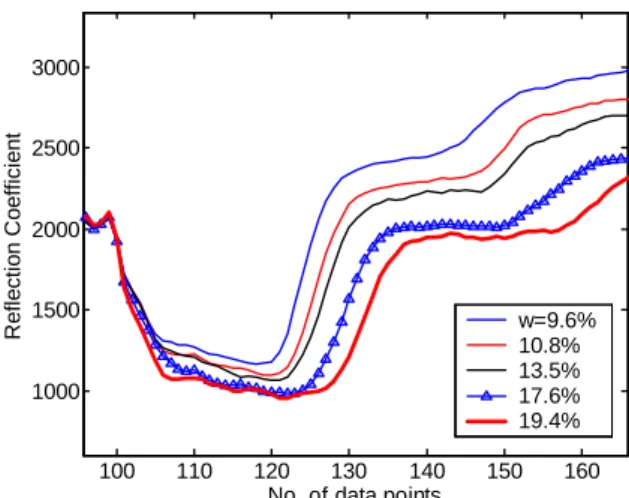
A silty sand (SM) was used for the simulated pene-tration tests. Seven different gravimetric water con-tents were used to prepare samples in a calibration chamber. The soil and water were mixed thoroughly to obtain the desired water content. The mixed soil was sealed with plastic wrap and allowed to equili-brate for more than 24 h, to yield a uniform soil specimen. The soil was then compacted in the cali-bration chamber in layers and the total mass of the soil and chamber was measured. Two TDR meas-urements were taken, one with the TDR penetrome-ter and the other with a multi-rod probe (MRP) simi-lar to Fig. 3(b). Then samples of the soil were oven-dried to determine the gravimetric water content. Tests were performed twice for each water contents to evaluate the repeatability.
The variation of TDR waveforms as the soil water content increases is shown in Fig. 11. The dielectric constant and electrical conductivity increases with water content, as can be inferred from Fig. 11. A good correlation between Kaand volumetric water
content (θ) exists as shown in Fig. 12. The correla-tion between σ and θ shown in Fig. 13 also shows great linearity. The Ka-θ relationship is relatively
independent of soil type and electrical conductivity of pore water (reference). But the σ -θ relation-ship greatly affected by pore water electrical con-ductivity. Therefore, apparent dielectric constant can be used for measuring volumetric water content (or void ratio when the soil is saturated). The volu-metric water content and electrical conductivity can then provide extra information for determining the characteristic of the pore water. Further research in-volves the dielectric spectroscopy of soils using the TDR penetrometer. The dielectric spectrum may add another dimension of information to the appar-ent dielectric constant and electrical conductivity. Detailed discussion of the use of electrical properties is beyond the scope of this paper.
100 110 120 130 140 150 160 1000 1500 2000 2500 3000
No. of data points
R e fl ec ti on C oeff ic ient w=9.6% 10.8% 13.5% 17.6% 19.4%
Figure 11. TDR waveforms for soils of different water contents.
15 20 25 30 35 2.6 2.8 3 3.2 3.4 3.6 3.8 4 4.2 θ % s qrt (K a ) R2=0.9453 data point linear regression
Figure 12. Correlation between Ka and θ .
15 20 25 30 35 0.04 0.05 0.06 0.07 0.08 0.09 0.1 0.11 0.12 θ % sq rt ( σ) R2=0.9721 data point linear regression
Figure 13. Correlation between σ and θ .
5.3 Effect of penetration
In addition to the measurements using the TDR penetrometers, TDR measurements were also per-formed using a MRP probe. The diameter of the multiple rods is 9.5 mm and the spacing between the center conductor and outer conductors is 65 mm. The effect of penetration on TDR measurements us-ing the MRP is considered negligible (Siddiqui et al. 2000). Comparing the measurements of TDR
pene-trometer with that of MRP can reveal the effect of penetration. The comparison is shown in Fig. 14
and Fig. 15 for Ka and σ , respectively. No sur-charge was added on top of the calibration chamber. Considering the low confining pressure, the soil in the simulated penetration test should be dilative. Hence, the void ratio increases due to probe inser-tion. The increase in void ratio results in a decrease in apparent dielectric constant and electrical conduc-tivity, as verified in Fig. 14 and Fig. 15. The effect of penetration is much more pronounced for electri-cal conductivity than for dielectric constant. This can be explained by comparing the spatial weighting function for electrical conductivity to that for dielec-tric constant. The change in dielecdielec-tric constant due to probe insertion is less than or comparable to the uncertainty associated with the K -a θ correlation in this case. This adds one more reason to why di-electric constant rather than di-electrical conductivity should be used for water content (or void ratio) measurements. The simulated penetration used a hammer to penetrate the TDR cone penetrometer. This may cause air gap between the penetrometer and soil. More comprehensive study and refined penetration test may be necessary to quantify the ef-fect of penetration in various cases.
0 5 10 15 20 25 0 5 10 15 20 25 K a fr om T D R pe ne tr eo m e te r K a from MRP R2=0.9880 data point linear regression 1:1 line
Figure 14. The apparent dielectric constant obtained from TDR penetrometer vs. that from MRP.
0 0.005 0.01 0.015 0.02 0 0.005 0.01 0.015 0.02 σ from MRP σ fr om T D R pen etr o m e ter R2=0.9919 data point linear regression 1:1 line
Figure 15. The electrical conductivity obtained from TDR penetrometer vs. that from MRP.
6 CONCLUSION
Time domain reflectometry is a promising tech-nique for simultaneously measuring the dielectric constant and electrical conductivity of a soil in situ. Current TDR probes can only apply to soils near ground surface. The paper describes the develop-ment of a TDR cone penetrometer that is capable of providing continuous TDR measurements during the cone penetration. Various probe configurations were experimentally studied. The data reduction method for the determination of apparent dielectric constant and electrical conductivity has been formu-lated and calibrated. The region of influence around the probe and the effect of penetration on TDR measurements are also studied. Research is under way to develop dielectric spectroscopy using the TDR penetrometer and new applications of this new technique. More work must also be undertaken to quantify and minimize the effect of probe insertion. ACKNOWLEGEMENTS
The research was sponsored by the National Science Council of ROC under contract numbers 89-2218-009-100 and 90-2611-E-009-004.
REFERENCES
Birchak, J.R., Gardner, C.G., Hipp, J.E. & Victor, J.M., 1974. High dielectric constant microwave probes for sensing soil moisture. Proceedings IEEE 62:93-98.
Baker, J. M. & Lascano, R. J. 1989. The spatial sensitivity of time-domain reflectometry. Soil Science 147:378-384. Dalton, F. N., Herkelrath, W. N., Rawlins, D. S. & Rhoades, J.
D. 1984. Time-domain reflectometry: simultaneous meas-urement of soil water content and electrical conductivity with a single probe. Science 224:989-990.
Fellner-Felldegg, J. 1969. The measurement of dielectrics in the time domain, Journal of Physical Chemistry 73:616-623. Giese, K. & Tiemann, R. 1975. Determination of the complex
permittivity from thin-sample time domain reflectometry: improved analysis of the step response wave form. Adv.
Mol. Relax. Processes 7:45-59.
Heimovaara, T. J. 1994. Frequency domain analysis of time domain reflectormetry waveforms: 1 measurement of the complex dielectric permittivity of soils. Water Resources
Research 30:189-199.
Knight, J. H. 1992. Sensitivity of time domain reflectometry measurements to lateral variations in soil water content.
Water Resource Research 28: 2345-2352.
Lin, C.-P. 2003. Analysis of a non-uniform and dispersive tdr measurement system with application to dielectric spectros-copy of soils. Water Resources Research 39(1): art. no. 1012.
Ramo, S., Whinnery, J. R. & Van Duzer, T. 1994. Fields and
Waves in Communication Electronics. 3rd ed., John Wiley, New York.
Topp, G.C., Davis, J.L. & Annan, A.P. 1980. Electromagnetic determination of soil water content and electrical conduc-tivity measurement using time domain reflectometry.
Site Characterization for the Investigation of Tunnel 8 Collapse
A.B. Huang, C.P. Lin, J.J.Liao, and Y.W. Pan
Department of Civil Engineering, National Chiao Tung University, Hsin Chu, TAIWAN
J. Tinkler
Hyundai Engineering & Construction Co., Ltd., Taiwan High Speed Rail Contract 230, Miaoli, Taiwan
Keywords: PMT, SPT, P-S logging, seismic refraction, resistivity, tunnel collapse
ABSTRACT: A section of the high speed rail tunnel collapsed before the installation of permanent lining. The section designated as Tunnel 8 was located in Miaoli County in Northern Taiwan. The resulting spoil blocked approximately 50 m of the tunnel. A crater of 28 m in diameter, with a maximum depth of 12.1 m was formed at the ground surface, at approximately 60 m above the crown level of the tunnel. A site charac-terization program was carried out to define the boundaries of the collapsed zone, provide ground water in-formation and stress and stiffness parameters for the outer and final concrete lining design. Six 100 m deep, rotary cored holes were drilled vertically from the ground surface, within the collapsed zone and penetrated through the tunnel level. SPT, pressuremeter and suspension P-S logging tests were performed in these bore-holes. Seven open boreholes, approximately 60 m deep, were drilled laterally from the concrete barricade at north and south end of the collapse zone within the tunnel at various angles. Geophysical tests which in-cluded seismic refraction tomography and resistivity tests were conducted from the ground surface. The data collected from the site characterization coupled with the geological background were analyzed and an image of the possible disturbance zone was created. The paper describes details of the site characterization, their in-terpretation and results of the analysis.
1 INTRODUCTION
The referenced tunnel was located near the pro-posed Miaoli Station in Northern Taiwan (see Figure 1) and part of Contract C230 of the high speed rail construction project that started in 2001. Sandstone with occasional layers of shale and mudstone of Pleistocene epoch, 4 – 5 million years of age, were the major rock formations in this region. The forma-tions intersected during the excavation of Tunnel 8 exhibit little to no structural complexity. Detailed tunnel geology prior to the collapse, interpreted from the regular face mapping showed that:
The weakest ground conditions encountered in Tunnel 8 occurred in the area of collapse. Loose sand, 4 to 6m thick, with pocket pene-trometer derived unconfined compressive strength was as low as 0.1 MPa, formed layers in the bench area, crown and above.
Perched water in mudstone layers, which caused falls of ground during the top-heading advance. This resulted from washing out of sand into the tunnel and subsequent
undermin-ing of the overlyundermin-ing mudstone and sandstone layers.
Perched water also caused migration of sand and silt from the bench to the invert during in-vert excavation. This caused self-mining of the bench and silting problems in the invert.
Observations have indicated that the mudstone exhibited a strength decrease from 1.5 to 0.5MPa when saturated. The sandstone showed a similar significant reduction in strength in the presence of water.
Minor jointing and reverse faulting has been mapped in the area.
Several falls of ground were recorded during the advance of the top heading through the area. The advancing North and South top headings
holed through inside the collapse zone, close to the Southern limit of the collapse at crown level. The induced loading as the two faces closed would have had some weakening effect on the inherently low strength rock mass.
The crown of Tunnel 8 was at 75m below ground surface (elevation 120m) and invert 85m. A col-lapse occurred in Tunnel 8 before the installation of
permanent lining, in the early hours of the morning on September 6, 2002. The resulting spoil blocked the tunnel at crown elevation from Chainage 107+560.70 to 107+613.40 representing 52.7m in extent from North to South. The collapse caused a crater to form at surface above the tunnel, centered 3.0m to the West of the tunnel centerline, approxi-mately 28m in diameter and a maximum depth of 12.1m. Concrete barricade was placed at the south and north ends of the collapsed zone soon after the event to prevent further expansion of the collapse. A site characterization program was carried out to define and determine the following:
The boundaries and geometry of the collapse zone above and surrounding the tunnel.
The elastic properties and densities of the for-mations within and outside the collapse zone, and an estimate of the coefficient of lateral earth pressure (Ko) of the disturbed ground around the tunnel.
Groundwater levels for the assessment of the post collapse water pressure around the tunnel, during and after rehabilitation.
Figure 1 The Taiwan High Speed Rail system.
This paper describes details of the site characteri-zation program, their interpretation and results of the analysis. Emphases will be placed on the first two items as information of groundwater levels mainly relied on readings from the observation wells.
2 SITE CHARACTERIZATION
The site characterization program consisted of seven rotary-cored holes from within and around the back-filled crater at surface. Standard Penetration Tests (SPT), P-S logging, and pressuremeter tests (PMT)
were performed in these boreholes and groundwater observation wells were installed upon field tests. A borehole location diagram and its relation with the crater resulting from the collapse are shown in Fig-ure 2. The topographic curves in FigFig-ure 2 are sepa-rated by 1m in elevation. Refraction Tomography was used in the early stage of exploration as a sur-face seismic method of investigation, with hydro-phones installed in boreholes to maximize data ac-quisition at depth. Due to poor signal retrieval during the Seismic Survey, it was decided to carry out a Resistivity Survey to complement the Seismic Refraction Tomography. A phase of inclined rotary coring and horizontal open-hole drilling was con-ducted from the concrete bulkhead in Tunnel 8 South.
Figure 2 Borehole locations
2.1 Drilling operation
Observation wells were installed in boreholes D2 and D3, and a single piezometer in boreholes D4 and D5. Borehole D6 was drilled to 100m deep from the “eye” of the collapsed zone. Borehole D7 was cored to a depth of 84m. The borehole orientation was surveyed with a down-the-hole camera and a 0 - 5° angle unit. The borehole (BH) top and bottom loca-tions according to these trajectories are presented on Figure 2. Pressuremeter tests were performed in D1 to D3 at depths from 60 to 100m. The air pressure inflated pressuremeter was equipped with strain gauged membrane expansion sensing arms to moni-tor the probe expansion. The PMT unload reload shear modulus values (Gur) are plotted in Figure 3. These Gur values correspond to a maximum strain difference of 0.5% during the unload reload tests. The Gur values above 90m were generally at 1 to 2 orders of magnitude smaller than those below 90m, indicating a clear boundary of the collapse zone.
Additional seven boreholes U01 to U07 were drilled with coring from the concrete barricade at the North end of the tunnel. U01 to U03 were oriented along the centerline of the tunnel, inclined at +10o to
0 10m Settlement Pin Inferred Fault BH Bottom Cracks Tunnel 8 BH Top N
+35° from the horizontal and drilled to depths of 57m to 65m. U04 to U07 were drilled to depths of 60m without coring, horizontally in a fan arrange-ment from the barricade face into the collapsed zone. These holes were drilled in an attempt to determine the boundary between the disturbed collapsed zone and the surrounding intact rock in the longitudinal axis of the tunnel. Figure 4 describes the orientation of boreholes U03 to U07 on a horizontal plan. Posi-tions of U01 to U03 on a vertical plan will be pre-sented later along with the estimated collapsed zone.
0 100 200 300 400 500 Gur, MPa 100 90 80 70 60 De pt h , m D1 D2 D3
Figure 3 Pressuremeter test results
Figure 4 Orientation of boreholes U03 to U07
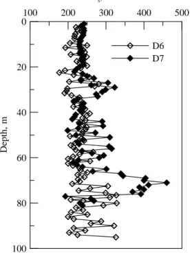
2.2 Geophysical Investigation
P-S Logging was carried out in boreholes D6 and D7, progressively at 1.0m intervals. The shear wave ve-locity (Vs) profiles from of P-S logging tests are shown in Figure 5. The plots indicate that the mate-rials throughout the measurement depth in D6 are
most likely disturbed to a point that they behave like sand. In D7 similar results were obtained except for certain depth ranges the Vs achieved higher values but were still lower than what would be expected from intact soft rock. The results indicate that D7 is slightly less disturbed than D6, which is to be ex-pected since D6 was drilled down the “eye” of the collapse. 100 200 300 400 500 Vs, m/s 100 80 60 40 20 0 Dep th, m D6 D7
Figure 5 Profiles of Vs in D6 and D7
Seismic refraction tests were carried out along three 115m long lines, two parallel to a line through D6 and D7 (A line), and one line (C line) normal to A line, through the collapsed zone at surface. The investigation was carried out in an attempt to deter-mine the extent and geometry of the collapsed zone in 3D using the tomography techniques. The results of these seismic investigation were inconclusive due to poor signal retrieval. It was suspected that loose surface material and ongoing surface drilling activity were the main cause of the poor test results.
Because of the undesirable seismic refraction test results, an electrical resistivity survey was carried out to map sub-surface changes. The material within the collapsed zone was expected to be highly dis-turbed and hence exhibit high porosity and perme-ability. The greater the degree of ground mass dis-turbance, the higher the permeability, lower degree of saturation, and hence higher resistivity. Thus there should be good resistivity contrast between in-tact (undisturbed) and the disturbed zone. The resis-tivity survey was carried out along lines A and C. The results are depicted in Figure 6.
3 DETERMINATION OF THE BOUNDARY AND SHAPE OF THE COLLAPSE
The initial tunnel collapse was interpreted as a “chimney cave” type of discontinuous subsidence
South portal Tunnel 8 U07 U06 U05 U03 U04
(Brady and Brown, 1993) which was characterized by large surface displacements over a limited surface area with very steep near vertical boundaries, with the formation of steps or discontinuities in the sur-face profile. Typically the sursur-face subsidence area of a “chimney cave” may be of a similar plan shape and area to the original excavation.
(a) Resistivity image for Line A
(b) Resistivity image for Line C Figure 6 Results of resistivity tests
The initial collapse on September 6, 2002 devel-oped through to surface very rapidly, around which circumferential subsidence tension cracks have sub-sequently developed up to 20m from the boundary of the initial crater.
Whilst the subsequent development of tension cracks can be partly interpreted as progressive sur-face failure into the original crater, their develop-ment was more likely a reflection of the progressive lateral extension of the disturbed zone around the ‘eye’ of the collapse. Accordingly a conservative in-terpretation was adopted with regard to the geometry and extent of the collapsed zone, and subsequent length of tunnel affected. The North and South boundaries were represented by a projection from the crown limits of the tunnel muck piles and the outermost tension crack at surface. These bounda-ries were vertical. The lateral limits, normal to the axis of the tunnel were similarly defined with angles from horizontal on the East and West of 80° and 85° respectively.
Significantly, it must be assumed that if there was progressive increase in the area affected by surface tension cracking, there would be an increase in the volume of disturbed material above the tunnel, and a corresponding increase in load. This increase can be monitored and accounted for through regular map-ping of the tension cracks, surface subsidence, incli-nometer and extensometer monitoring.
There was no observable damage to the crown support on the North side. There was therefore a possibility that the actual limit of tunnel crown break is some distance to the South, and hence a reduced length of tunnel affected by the collapse was as-sumed.
3.1 Core Logging Interpretation Problems
Problems encountered in logging the site investiga-tion core and the subsequent interpretainvestiga-tion of the geology, ground conditions and boundaries included: The inherently low rock mass strengths of the
material being cored even in a relatively undis-turbed state.
The core quality and recovery was undoubtedly affected by the disturbance due to SPT testing, which could also disturb formations at the bot-tom of the borehole
The usual methods of rock mass quality as-sessment such as RQD, Fracture Frequency and the Condition of Discontinuities could not be applied to these cores from inherently very weak and subsequently disturbed formations. Poor core recoveries and core losses have made
geological interpretations difficult, particularly from tunnel crown to below the invert level. Consequently information from a combination of borehole logging, previous tunnel mapping and recent invert mapping was used to refine the profile normal to the tunnel axis at lower elevations.
A visual qualitative assessment of rock quality was attempted,
The collapsed zone was still settling and under-going compaction. This process compounded the day-to-day drilling operational problems, which subsequently affected: core quality and recovery, casing installation and removal, in addition to affecting overall drilling progress. The data from the PMT, P–S Logging and
Re-sistivity Tomography above invert level; indi-cated that essentially all holes were drilled in disturbed ground.
Borehole deviation affected the accurate projec-tion of data on to the relevant profiles.
3.2 Geometry of the Collapsed Zone
The geometry of the collapse and length of tunnel affected were interpreted from the following infor-mation:
The limits of the muck piles at crown eleva-tions on the North and South sides of the tunnel. The mapped location of the surface tension
cracking.
The projection of the limits of the muck piles to the plan locations of the cracks at surface.
The Resistivity Tomograms from which a qualitative assessment of the boundaries and shape of the disturbed zone was derived.
D6
D6 D7
The results of the borehole geological and geo-technical logging, and the fact that the PMT, P– S Logging and to a lesser extent resistivity to-mography, indicated that essentially all bore-holes were drilled within disturbed ground above invert level.
3.3 Cross Section Normal to the Tunnel Axis
The information used to determine the boundaries of the collapsed zone in cross section normal to the tunnel axis is as follows:
The center of the collapsed zone at surface was used to define the center of the collapse in cross section. This provided the focus around which the geometry of the collapsed zone could be de-fined in 3 dimensions, and corresponds to the location of the excavation activity in Tunnel 8 South at the time of the collapse.
The geological interpretation of the logging of boreholes D4 and D5, together with the pro-jected information from D1. In particular the mudstone layer that acted as a “marker” be-tween 18 and 21m below ground surface, and the boundary between sandstone and mudstone at 37 – 39m which showed a displacement of +/- 12m at the ‘eye’ of the collapse, which co-incidentally was equivalent to the depth of the collapsed zone at surface.
Geotechnical and down-the-hole testing results from boreholes D4, D5 and D1, including SPT test results, core recoveries and a qualitative as-sessment of disturbed zones.
The plan limits of the surface subsidence ten-sion cracks.
The SPT ‘N’ values in D4 between 42m and 67m depths show a significant reduction compared with those values over the same interval in D5. In addi-tion the core recoveries are correspondingly lower and there was a greater frequency of interpreted dis-turbed zones in D4 than D5 over the same interval. This reflects the fact that D4 was closer to the “eye’ of the collapse zone
High SPT ‘N” values and core recoveries, favor-able bedding intersection angles in the mudstone core together with favorable PMT results in D1 at 93m indicated that there was little to no extension of the disturbed zone below the invert level. Local high ‘N’ values, in D1 in the ‘eye’ of the collapse, were interpreted as local isolated denser / stiffer lay-ers or blocks within the collapsed column. The SPT ‘N’ values, together with the interpreted boundaries of the collapsed zone are presented on Figure 7. 3.4 Longitudinal Section Along the Tunnel
Centerline
The information used to define the boundaries of the collapsed zone in longitudinal section along the tun-nel centerline is as follows:
Recognition of the mudstone ‘marker’ in bore-holes D1, D2, D3 and D7 and its displacement associated with the ‘eye’ of the collapse
The location of bent roof pipes was taken as the Southern limit at crown level.
Bent and damaged pipes were not evident at crown level in T08 North. The contact of the muck pile with the crown was interpreted as the Northern limit at crown level.
Plan limits of the surface subsidence tension cracks.
The P–S Logging test results indicated that D7 was drilled in disturbed ground, notwithstand-ing the fact that its trajectory indicated that it did not intersect the tunnel.
Figure 7 Collapse boundaries normal to the tunnel axis
Cored boreholes U01, U02 and U03 were drilled early in the site investigation from the South bulk-head. They were prematurely terminated at depths still within the disturbed zone.
The SPT ‘N’ values together with the interpreted collapsed zone are presented on Figure 8.
D5 D1 D4 Elevation, m Interpreted collapse boundaries D6
Figure 8 Collapse boundaries along the tunnel Centerline
4 GROUND CONDITIONS ASSOCIATED WITH THE COLLAPSED ZONE
4.1 Open Hole Drilling
This phase of the investigation included boreholes U04 to U07 using a hydraulic feed rotary rig. The following observations were made from the data of the open-hole drilling:
Penetration rates vary, indicating the heteroge-neity of the rock types in the caved column. The change in color of the flush enabled a
lim-ited interpretation of the geology, which showed variability, again indicating the hetero-geneous nature of the collapsed material.
Flush returns were generally good 80 – 100% but with a few local zones intersected up to 3m with 0% returns, and 1 – 2m with 20, 30 and 50% returns. The zones of 0% flush returns probably indicate very loose material, possibly voids, although this did not reflect in the pene-tration rates, due to the type of drilling rig util-ized. Zones of 0% flush returns were logged in U06 at 22m – 23m and 27.5m – 30.5m, with 20% between 21.5m – 22m and 57.4m – 57.5m, 30% 57.5m – 58.5m. A zone of 30% returns was logged in U05 between 21.7m – 23m. Other than the bulkhead concrete, no concrete
and/or steel was intersected in any of the holes during the horizontal drilling phase.
The geology interpreted from flush returns colour is presented on Figure 3.
4.2 Surface Drilling
Information from the coring within the collapsed zone down to invert level indicated very poor ground conditions. This was evidenced by very low SPT ‘N’ values; locally poor ground conditions of-ten precluding SPT testing, very low and ofof-ten zero core recovery.
SPT ‘N’ values varied with depth depending on the location of the individual hole collar at surface and its proximity to the focus of the collapse. SPT ‘N’ values could vary from low values to refusal, in-dicating the variability of the density and stiffness of the material in the caved column, reflecting a com-bination of on-going compaction, and the possible presence of isolated blocks of separate sandstone and mudstone within the caved column particularly at lower elevations.
The SPT ‘N’ values in D4 and D5, showed a gen-eral increase in value with depth as the borehole de-viated further away from the “eye” of the collapse. Similarly SPT ’N’ values in boreholes D1, D2 and D3 below the invert level showed an increase, often refusal, with depth.
4.3 Cavities
The minimum cavity dimension, which could be determined by the Resistivity Tomography was 2.5m, which was equivalent to half the electrode spacing used in the investigation. Cavities would be indi-cated by very high zones of resistivity on the tomo-grams, many orders of magnitude greater than those shown. There were no zones of abnormally high re-sistivity delineated on the tomograms as shown in Figure 6. The highest recorded value was < 1000 Ohm/m, reflecting a “wet” sandstone type material. The inference was therefore, that there were no cavi-ties > 2.5m above the crown level, within the area defined by the investigation.
No cavities were identified in the collapse zone above crown level during the drilling and logging of D1, D2 and D3.
However cavities were identified from the surface drilling within the zone between tunnel crown and invert levels in D2 from 83.55m to 84.90m and D3 80.60m to 81.80m.
4.4 Between Crown and Invert Level
From the limited information available from boreholes D1, D2 and D3 the following observations were made with regard to the general ground condi-tions above invert level:
Lattice arch steel and shotcrete with steel mesh reinforcing intersected in boreholes D1 and D2 between top heading floor and tunnel invert level, and in D3 between crown and top head-ing floor. Elevation, m Interpreted collapse boundaries D7 D2 D1 D3