科技部補助專題研究計畫成果報告
期末報告
多變量複合卜瓦松跳躍擴散模型與高頻資料下之選擇權評價與
投資組合策略之研究(第2年)
計 畫 類 別 : 個別型計畫 計 畫 編 號 : MOST 102-2410-H-004-042-MY2 執 行 期 間 : 103年08月01日至104年10月31日 執 行 單 位 : 國立政治大學金融系 計 畫 主 持 人 : 廖四郎 計畫參與人員: 博士班研究生-兼任助理人員:陳俊洪 處 理 方 式 : 1.公開資訊:本計畫涉及專利或其他智慧財產權,2年後可公開查詢 2.「本研究」是否已有嚴重損及公共利益之發現:否 3.「本報告」是否建議提供政府單位施政參考:否中 華 民 國 104 年 12 月 30 日
中 文 摘 要 : (第一年)
本文利用一個多變量複合卜瓦松模型(Multivariate compound Poisson diffusion model)來描述資產價格的動態過程,此模型不 僅能解釋資產跳躍亦能解釋資產間共同跳躍情況,並利用Esscher測 度轉換得到一個風險中利的資產動態過程,並將此模型應用到互換 選擇權評價來探討共同跳躍對於選擇權評價之影響。研究發現當資 產間共同跳躍次數愈高,選擇權價值愈高。 (第二年) 隨著資產間的共同移動與共同跳躍的現象加劇,過去建構在資產動 態服從幾何布朗運動的情況將無法描繪。本文提出一個多變量複合 卜瓦松跳躍擴散進一步捕捉資產間的共同移動現象,同時也將共同 跳躍的現象納入到模型中,並透過Markovwitz的平均數-變異數法則 來建構投資組合。研究結果發現當共同跳躍次數的增加,將增加資 產間的相關係數,這使得投資組合的風險分散的效果遞減,此外 ,當有重大的系統性風險發生時,共同跳躍的次數也會增加,且當 共同跳躍的頻率增加至某一程度時,資產間的相關係數將達到1,此 時,投資組合的建構將無法達到風險分散的效果。 中 文 關 鍵 詞 : 共同跳躍、平均數-變異數法則、多變量複合卜瓦松跳躍擴散 英 文 摘 要 : (First Year)
In this study, we investigate the valuation of European exchange options under a two-asset jump-diffusion process with correlations, where both individual jumps and cojumps in the underlying stock price dynamics are modeled by two independent compound Poisson processes with log-normal jump sizes. The Esscher transform technique is applied to
provide an efficient way for exchange option valuation under an incomplete market setting. The estimated results and numerical examples are provided to illustrate the impact of cojumps on option prices.
(Second Year)
The phenomena of co-movement and co-jump among assets become more and more frequent and result in the dynamic process built basing on the geometric Brownian motion cannot depict these anymore. For the sake of taking co-movement and co-jump among assets, we propose a new process called multivariate compound poisson diffusion model to more accurately model the dynamics of asset price. In addition, we use the mean-variance method proposed by Markovwitz to construct the portfolio and investigate the impacts of the co-jump on the portfolio construction. We find the increasing of co-jump intensity will also increase the correlation between assets and result in decreasing the effect of risk diversification through portfolio
construction. Further, we also find the major systematic risk occurs, such as subprime crisis, the intensity of co-jump will also increase.
英 文 關 鍵 詞 : Co-jump, mean-variance, multivariate compund poisson jump diffusion,Esscher transform
(多變量複合卜瓦松跳躍擴散模型與高頻資料下之選擇權評價與投資組合策略之
研究第一年)
Cojump phenomena and their impacts on exchange option pricing
☆Abstract
In this study, we investigate the valuation of European exchange options under a two-asset jump-diffusion process with correlations, where both individual jumps and cojumps in the underlying stock price dynamics are modeled by two independent compound Poisson processes with log-normal jump sizes. The Esscher transform technique is applied to provide an efficient way for exchange option valuation under an incomplete market setting. The estimated results and numerical examples are provided to illustrate the impact of cojumps on option prices.
JEL classification: C58; G12
Keywords: European exchange option; Two-asset jump-diffusion process; Cojump; Esscher transform
1. Introduction
Many derivative contracts traded in exchanges and in over-the-counter markets, such as exchange options, have payoffs depending on more than one asset and are most commonly used in stock markets and foreign exchange markets. For pricing exchange options explicitly and practically, a necessary step is to establish a dynamic model for the asset fluctuations. Margrabe (1978) initially introduces the pricing formula for an exchange option, in which the pure diffusion dynamics of both stock prices are log-normal with correlated Wiener processes. In addition, Bjerksund and Stensland (1993), Broadie and Detemple (1997), and Lindset (2007) show the pricing formulas for the American exchange options. Nevertheless, increasing empirical evidences have revealed that the geometric Brownian motion is not completely consistent with the reality. In other words, there exist empirically observed jumps or extreme events in stock prices (Eraker et al., 2003; Eraker, 2004; Maheu and McCurdy, 2004). Although the price behavior for a single asset is already known to jump individually, the occurrence of cojumps for both asset prices is also possibly existed (Chan, 2003; Lu et al., 2010; Lahaye et al., 2011; Dungey and Hvozdyk, 2012). Cojump refers to the presence of simultaneous discontinuities in two asset price series. In view of the aforementioned literature, this study proposes a dynamic model for two asset prices with illustrating such a cojump phenomenon, in which the
cojump event is governed by a bivariate compound Poisson process with a log-normal jump size. The model captures not only the existence of jump phenomena but seems to generally describe the cojumping behavior of two asset prices as well.
The datasets used in the descriptive analysis of Table 1 and Table 2 consist of the multiple daily stock prices. Analyzing stock returns makes us to investigate the potential effects of different jump behaviors. Table 1 and Table 2 show several significant jumps of 30 components of the Down Jones Industrial Average (DJIA) in the daily data1 after the U.S. subprime financial crisis and before this turmoil. Furthermore, we also find evidences of cojumps between the 30 components in Table 3 and Table 4. A further implication of Table 3 and Table 4 is that in the sample data the jumping and cojumping behavior of two stock prices could happen over time. More specifically, the global financial turmoil does really have influence of changing the jump relation between two asset prices.
[Insert Table 1–4]
A bivariate Poisson distribution is a well-known bivariate discrete distribution (Holgate, 1964). It is appropriate for modeling paired counting data with correlation. In the case of a cojumping, the simultaneous jumps of two stock prices cannot be
1 The empirical data are from Yahoo Finance and cover the period from 3 January 2005 to 31 December 2010.
considered independently. In this situation, a bivariate compound Poisson distribution is more appropriate when the counting distribution is bivariate Poisson and the size distribution is bivariate for the claim (Hesselager, 1996). In this study, instead of using constant arrival intensity under a pure Poisson process used in the Merton-type jump-diffusion process (Merton, 1976), we set the jump components of both stock prices to be a bivariate compound Poisson process whereby the intensity processes of individual jumps and cojumps are modeled at the same time.
Motivated by our empirical evidences in Table 1 and Table 3, in order to capture various ways of individual jumps and cojumps in stock prices generated by the actual market simultaneously, we model the price dynamics of two stocks by identifying a two-asset jump-diffusion process with both individual jumps and cojumps. Under such a dynamic process, the stock price can be decomposed into two parts, a continuous diffusion part driven by a two-dimensional geometric Brownian motion and a jump part with jump events modeled by a bivariate compound Poisson process where there are both individual jumps and cojumps. More exactly, if a jump event
corresponds to an individual jump of the ithstock price, then only the ith stock price will jump; otherwise, if a jump event corresponds to a cojump, then both stock prices will jump with a positive probability. This dynamic model therefore provides a flexible framework to study the individual jumps and cojumps for both stock prices.
The market is incomplete in such a two-asset jump-diffusion economy, and we therefore make use of Esscher transform technique adopted from Gerber and Shiu (1994). By relaxing the assumption of a non-systematic jump risk (Merton, 1976), we select a pricing kernel and determine the Esscher parameters (risk premiums) for option valuation. In this study, we show that even in the presence of individual jumps and cojumps for both stock prices, the price of an European exchange option can be derived using the specific approach of Esscher transform.
This study makes three major contributions. First, it extends the relevant empirical literature by identifying the existence of individual jumps and cojumps in stock prices. The empirical evidences are significant for considering such phenomena in paired stock price modeling. Next, it extends the growing empirical literature on the jump behaviors of stock prices in the actual market. Analyzing these behaviors is critical for understanding the operation of the stock market and the risks involved. Finally, it extends the pricing literature on the valuation of European exchange options for an economy with non-systematic jump risks and takes the systematic risks of both individual jumps and cojumps into consideration in pricing European exchange options.
Section 3 illustrates the risk-neutral pricing measure and the generalized exchange option pricing formula. In Section 4, we provide the empirical and numerical results. Section 5 concludes this study.
2. Model framework
As shown in Table 1 and Table 3, the individual jumps and cojumps do exist in stock price realizations. Therefore, we use a bivariate jump-diffusion process to model the stock prices. Let
, ,F P
be a complete probability space, where P is the physical probability measure. A two-asset jump-diffusion process for the stock prices at time t, S ti( ), can be set as( ) , 1 ( ) ( ) exp 1 ( ) i N t i i i i i i i j i j dS t dt dW t d Y S t , i 1, 2, (1)
where the appreciation rate i and the volatility i of the stock i are constants,
( )
i
W t is a two-dimensional Wiener process with correlation under P. The jump risk components are indicated by a bivariate Poisson process N t with the constant i( ) arrival intensity i , and the jump sizes are supposed to follow a log-normal distribution as in Merton (1976).
Yi j, : j1, 2,...
are the jump sizes of the stock iwhich are assumed to be independently identically distributed random variables. If a jump event occurs at time j , the jump size Yi j, is normally distributed with mean
i
u and variance i2. Therefore, the mean percentage jump size of the ith stock
price is exp , 1 exp 1 2 1 (1) 1
2 i
i E Yi j ui i Y . In Eq. (1), we also
assume that all of the random variables W ti( ), N ti( ) , and Yi j, are mutually
independent.
Considering the case of two correlated stock prices, we suppose that the two jump terms N t1( ) and N t2( ) are partially correlated, meaning that if one stock price jumps then the other will jump with a probability p. We construct them in such a manner using three independent Poisson processes denoted by n t , 1( ) n t , and 2( )
( )
c
n t . The independent Poisson process n t has intensity i( ) i with discrete
probability density function as follows:
( ) exp ! g i i i t P n t g t g , (2)
for i
1, 2 . We define N ti( )n ti( )n tc( ) and N ti( ) Poisson
i c
. In other words, there are two types of jumps, individual jumps only for the ith stock price with the arrival intensity i and cojumps with the arrival intensity c, for both stock prices. The Poisson processes N t1( ) and N t2( ) are able of producing the individual jumps through n t and 1( ) n t , as well as the cojumps through 2( ) n t . A c( ) change of variables and integrating out n t result in the joint probability density c( )function for N t1( ) and N t2( ), which is given by 1( ) , 2( ) P N t m N t n min , 1 2 1 2 0 exp ! ! ! m n m v n v v c c v t t t t m v n v v , (3)
Hence, Eq. (1) can be rewritten as
( ) ( ) , 1 ( ) ( ) exp 1 ( ) i c n t n t i i i i c i i i i j i j dS t dt dW t d Y S t , (4) for i1, 2.
3. Change of measures and option pricing
The security economy defined by Eq. (4) is incomplete, this means that, under the assumption of no arbitrage opportunities in this market, there are infinitely many equivalent martingale measures with which to price options. We therefore need to determine a risk-neutral pricing measure Q. This implies changing the probability
measure linked to the two-asset jump-diffusion process so that both stock prices discounted at the risk-free rate are Q-martingales. In such a two-asset jump-diffusion
economy, we employ the Esscher transform developed by Gerber and Shiu (1994; 1996) to select the martingale pricing measure for pricing European exchange options.
3.1. Esscher transform for the two-asset jump-diffusion process
Relaxing the model assumptions of Merton (1976), and applying the Esscher transform for the two-asset jump-diffusion process we then determine a risk-neutral pricing measure. For i
1, 2 and all t
0,T , we decompose the two-asset jump-diffusion log-return process Z ti( ) log S ti( ) /Si(0) C ti( ) J ti( ) J t c( ) into a continuous diffusion part ( ) 1 2 ( )2
i i i i i c i i i
C t t W t , an
individual jump part ( ) , 1 ( ) n ti
i j i j
J t Y , and a cojump part ( ) ,
1 ( ) n tc c j i j J t Y . Here, let Wi t F and Ni t
F be the P-augmentation of the natural filtrations generated by ( )
i
W t and N t , respectively, and define i( ) Wi Ni Wi ni nc
t t t t t t
F F F F F F as the
- algebra for each t
0,T . Under a filtered probability space
0, , , ,F P Ft t T ,
the Radon-Nikodym derivative of the Esscher transform is formally given by
0 exp ( ) ( ) exp ( ) i i W t i C h i i h C F i i F h W t dQ t dP E h W t 0 0 ( ) ( ) , , 1 1 ( ) ( ) , , 1 1 exp exp exp exp i c i c i c i c ni nc n t n t J J i j i j j j n t n t J J i j i j F F j j h Y h Y E h Y E h Y e x p ( )1 ( 2 ) 2 i i C C i i i h W t h t
( ) ( ) , , 1 1 exp exp i c Ji Jc i c n t n t J h J h i j i i i j c i j j h Y t h Y t , (5)
where Qh is called the Esscher measure and hRn for
C J Ji, i, c
, wherei C
h , hJi , and hJc are the Esscher parameters of ( )
i
C t , J ti( ) , and J t , c( )
respectively. As a consequence, the mean percentage jump size becomes 2 , 1 exp 1 exp ( ) 1 ( ) 1 2 Ji i i i i i J J J J h i E h Yi j h ui h i Y h . Furthermore, the
Esscher transform density process h ( )t is an exponential Ft-martingale.
In line with the general option pricing theory, the existence of a risk-neutral pricing measure is equivalent to the non-existence of arbitrage trading strategies that replicate option payouts (Harrison and Pliska, 1981; 1983). Thus, under a risk-neutral pricing measure, the driving two-asset jump-diffusion process for two correlated stock prices is an Ft- martingale. It is possible to select the risk-neutral Esscher measure as
the measure Qh such that the discounted stock price processes are Qh-martingales. This is obtained by determining the Esscher parameters hCi , hJi , and hJc as
solutions of Eh exp rt S t Fi( ) 0 Si(0). Let the Esscher transform be defined by
Eq. (5), then the martingale condition is satisfied if and only if
2 i C i i i c i i r h (6)
2 1 2 i J i i u h
(7) and 2 1 2 c J i i u h . (8)
Appendix A shows the detailed proof.
An equivalent martingale measure can be treated as the Esscher measure Qh with respect to the measure P. We begin with identifying the dynamic process for
two correlated stock prices under the risk-neutral pricing measure Qh . Let hCi, hJi,
and hJc be the Esscher parameters of the risk-neutral Esscher measure, then under
h Q and conditional on Wi t F , ( ) ( ) Ci h i i i W t W t h t, (9)
is a Wiener process. Furthermore, under Qh , the arrival intensities ih and ch of the Poisson processes nih( )t and nch( )t , and the jump size Yi j,h are respectively given by 2 1 ( ) exp 2 i i i i J J J h i i Y h i h ui h i , (10) 2 1 ( ) exp 2 i i i i J J J h c c Y h c h ui h i , (11)
and
. . . 2 2 , i , i i d J h i j i i i Y N u h , (12) where h ( ) ( ) Ci i i iW t W t h t is changed by the Esscher transform, which means that the investors receive a premium Ci
i
h
for the continuous diffusion risk at time t ,
and the Wiener process is affected by the measure change. Through the change of
measures, the jump risk can be formulated by the Esscher transform intensities ih and ch of the Poisson processes nih( )t and nch( )t . For i
1, 2 , the arrival intensities ( i) i J h i i Y h and i( i) J hc c Y h are altered by the Esscher
transform, which means that the investors receive a premium ( i)
i
J
Y h for the jump
risk at time t , and thus the arrival intensity is affected by the measure change. If ( i) 1
i
J
Y h , the jump risk is not priced as in Merton (1976), and the arrival intensity
and distribution are unaffected by the measure change. Under Qh, if a jump event occurs at time j, the jump size Yi j,h is normally distributed with mean Ji 2
i i
u h
and variance i2. Appendix B presents the detailed proof.
Using the solutions of Esscher parameters given by Eqs. (6)–(8), we have
( ) ( ) h i i i c i i i i r W t W t t , (13)
2 2 2 exp 8 2 h i i i i i u , (14) 2 2 2 exp 8 2 h i i c c i u , (15) and . . . 2 2 , 1 , 2 i i d h i j i i Y N , (16) where i i i c i i r and 2 2 2 exp 8 2 i i i u
are the market prices of the
continuous diffusion risk and jump risk at time t , respectively. In addition, under
h
Q , the jump size Yi j,h is normally distributed with mean 1 2
2i
and variance i2.
Consequently, the two-asset jump-diffusion process for both stock prices under Qh is ( ) ( ) , 1 ( ) ( ) exp 1 ( ) h h i c n t n t h h i i i i j i j dS t rdt dW t d Y S t , i 1, 2,
(17) where Ci 2 h hJi h hJi i i i c i i i i c i r h for all t
0,T .3.2. Pricing European exchange options in a two-asset jump-diffusion economy
one stock to another stock. More precisely, the payoff of an exchange option is
1 2
( ( )S T KS T( )) , where K is the ratio of the shares to be exchanged. Under the assumption that there are no arbitrage opportunities in the market, we price European
exchange options under the risk-neutral pricing measure Qh . In a two-asset jump-diffusion economy, the price of an European exchange option at time zero is given by min , 1 2 1 2 0 0 0 exp ! ! !
(0)
h i m v n v v h h h m n c h h h c m n v T T T T m v n v vC
S1(0)N d1,m n, KS2(0)N d2,m n, , (18)where ih denotes the arrival intensity of the Poisson process nih( )T , m and n denote the numbers of jumps for N1h( )T and N2h( )T in the time interval
0,T . In addition, N( ) denotes the cumulative distribution function of a standard normalrandom variable and
2 1 1, , 2 2 2 1 2 2 2 2 1 1 2 2 1 ln 2 (0) (0) m n m d T m n S T m n KS (19) 2 2 2 2,( , )m n 1,( , )m n 1 2 d d T m n (20) and
2 2
1 2 2 12 1 2 . (21)
Eq. (18) can be viewed as the weighted sum of an expected European exchange option with weights being the joint probability of Poisson jumps. It is clear that the correlations between the two stocks also have impacts on the option prices. Appendix C gives the detailed proof.
We further illustrate the properties of the generalized exchange option pricing formula by considering several special cases with their specific formulas in the following examples. If ( i) 1
i
J
Y h , which implies that no premium is paid for the
jump risk, as in Merton (1976). Hence, Eq. (18) can be reduced to
min , 1 2 1 2 0 0 0 exp ! ! !
(0)
i v m v n v m n c c m n v T T T T m v n v vC
S1(0)N d1,m n, KS2(0)N d2,m n, , (22)If K1, Eqs. (18) and (22) are the solutions of a regular exchange option under the different jump risk considerations (systematic and non-systematic jump risks), respectively. If K1 with the absence of jumps, Eq. (18) reduces to the pricing formula of Margrabe (1978) in the Black–Scholes framework, which is given by
1 1 2 2
(0) (0) (0)
BS
where 2 1 1 2 1 ln 2 (0) (0) T d T S S (24) 2 1 d d T (25) and 2 2 1 2 2 12 1 2 . (26)
4. Empirical results and numerical illustrations
In this section, we take two financial institution of American bank (denoted as BAC) and J.P. Morgan Chase company (denoted as JPM) of the 30 components of the Down Jones Industrial Average (DJIA)2as example to investigate the suitability of traditional geometric Brownian motion model and the proposed cojump model to the market data and the impact of cojump on exchange option and its difference during the period of pre- and post- subprime crisis.
4.1. Empirical results
The summary statistics of the return of the underlying stock price listed in Table 1 and Table 2 shows the distribution of return of the 30 component of DJIA is not
2 The purpose of taking these two financial institution as example lies in the financial institution suffering the most during the subprime crisis.
normal in the point of view of the coefficients of skewness and kurtosis. Furthermore, taking the three standard deviation of individual return as a criterion of jump, we can tell the jump and cojump phenomena exists and the jump and cojump is more frequent in the period post- crisis than it in the pre-crisis from Table 3 and Table 4, such as the the number of jump of BAC in post-crisis is 11 is larger than 6 in the pre-crisis and number of cojump between BAC and JMP in the post-crisis is 7 is also larger than 4 in pre-crisis. The discussions about the Table 1, Table 2, Table 3 and Table 4 shed doubts on the validity of the geometric Brownian motion and the jump-diffusion model introduced by Merton (1976). Motivated by these findings we investigate the capability of a two-asset jump-diffusion process for modeling two correlated stock prices. In the empirical analyses, we take the American bank (denoted as BAC) and J.P. Morgan Chase company (denoted as JPM) as an example for illustrating the impact of cojump on exchange option pricing during and before the subprime financial crisis and denote S1 and S2 being JPM and BAC, respectively. We show
the estimated results using actual market data from the Yahoo Finance and use the traditional Black–Scholes model as a benchmark for the actual data analyzed.
The estimated parameters and corresponding standard errors (the latter in parentheses) after and before the subprime financial crisis are respectively reported in Table 5 and Table 6. These tables provide several interesting results. After the turmoil,
the individual jump intensity 1 is 0.0053 larger than 0.0027 before the crisis for
BAC, while JMP’s intensity behaves just in the opposite way. However, the cojump intensity C after the turmoil is 0.0093 larger than 0.0053 before the crisis.
Furthermore, the volatilities of Brownian motion (0.0378 for BAC and 0.0342 for JPM) and jump (0.1915 for BAC and 0.1498 for JPM) after the turmoil are also respectively larger than those (: 0.0089 for BAC and 0.0109 for JPM, : 0.0356 for BAC and 0.0425 for JPM) before the crisis. It reveals that after the crisis the assets seem to be more volatile. Furthermore, we can find the likelihood ratio test 3(Hereafter denoted as LRT) show the proposed cojump dominates the BSM in the
both post- and pre- crisis period in Table 5 and Table 6 under the 95% confidence level.
[Insert Table 5–6]
4.2. Numerical illustrations
In this section, we evaluate the exchange option prices for pre-crisis and post-crisis periods. As a benchmark, we apply the Black–Scholes model (BSM) to 3
2 1 , 1 0) ( ) ( ln( 2 r asy U R L LLRT is for test the null hypothesis and alternative hypothesis Holds Model BSM : 0
H H1:Theproposed cojumpmodelHolds and LR(0) and LU(1) are
likelihood function of the restricted and unrestricted model, respectively.The r is the degree of freedom and equals to the number of parameters difference between the restricted and the unrestricted model. If
LRT is significant large by comparing it with the 100(1-) percentile point of the Chi-Square with degrees of freedom 2
1 ,
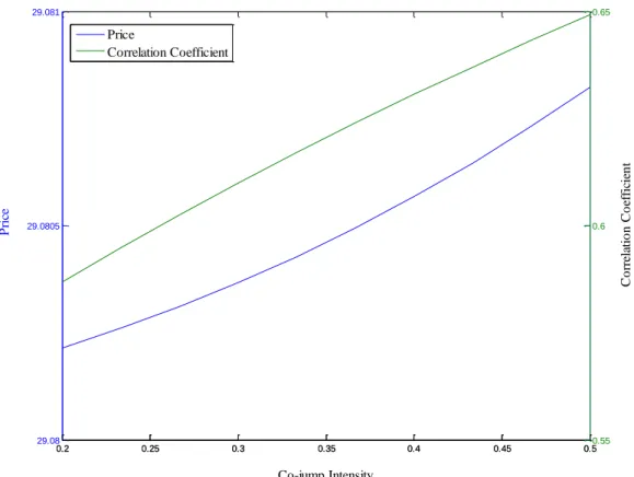
price European exchange options. Here we calculate the exchange option prices using the estimated parameters in Table 5 and Table 6 and the initial stock prices of the BAC and JPM after the subprime financial crisis are 13.34 and 42.42 at 31 December 2010, respectively. In addition, the initial stock prices of BAC and JPM before the subprime financial crisis are 41.26 and 43.65 at 31 December 2007, respectively. In addition, we use one-year U.S Treasury yield rate as a proxy for risk free rate (the risk free rate for post-crisis and pre-crisis are 0.0029 and 0.0334, respectively). Accroding to Table 7, we can find the difference between closed-form solution and simulation is very trivial, and this verifies the validity of the derived closed-form formula of cojump-diffusions applied in exchange option pricing. In addition, there is no big difference between the Merton measure and the Esscher measure. This may due to the jump premium simultaneously considered in the esscher measure for both asset and offset the jump premium effect on exchange option price. The last, we conduct scenario analyses to analyze the influences of the changing cojump intensity on the exchange option prices. The increasing cojump intensity would increase the exchange option prices as in Figure 1. This result is also match the original conclusion of equation (23), the larger correlation coefficient between two assets, the higher the exchange option price.
[Insert Fig. 1]
5. Conclusions
In this study, we empirically investigate the presence of individual jumps and cojumps in stock prices. The empirical data show that the two correlated stock prices are better approximated by two-asset jump-diffusion processes with both individual jumps and cojumps. Compared with the existing jump-diffusion processes (Merton, 1976; Kou, 2002), the main contribution of this article is that we incorporate cojump risks into the continuous-time stochastic process. According to the empirically favored two-asset jump-diffusion processes for the underlying stock prices under the incomplete market setting, we use the Esscher transform to identify a risk-neutral pricing measure for valuing European exchange options. After determining the risk premiums, we further derive the generalized exchange option pricing formula and demonstrate that the solution under the non-systematic jump risk assumptions of Merton (1976) and the pricing formula of Margrabe (1978) are special cases of the generalized pricing formula. We conclude that a bivariate Poisson process can explain more the cojump phenomena than a single Poisson process when pricing European exchange options and the relationship between cojump intensity and exchange option price is positive.
Appendix A: Solving the Esscher Parameters
Proof. Let Eh denote the mathematical expectation operator with respect to the Esscher measure Qh equivalent to P. Applying Eq. (5), we have
0 0 (0) exp ( ) exp ( ) h h i i i dQ S rt E S t F rt E S t F dP ( ) ( ) 2 , 1 1 (0) exp ( ) 2 i c n t n t h i i i i i c i i i i j j dQ S E r t W t Y dP 2 2 2 1 1 1 (0) exp 1 2 2 2 i i C C i i i i i c i i i S r t h t h t exp 1 exp 1 Ji Ji Jc Jc h h h h i i i t c i i t , (A.1)
From the mutual independence of random shocks W ti( ), N ti( ), and Y , and then i j,
the martingale condition Eh exp rt S t Fi( ) 0 Si(0) holds if and only if the
Esscher parameters hCi, hJi, and hJc satisfy
2 0 i C i r i i c i h i (A.2) 2 2 1 0 2 i J i i i u h (A.3) and
2 2 1 0 2 c J i i i u h , (A.4)
for all t
0,T . Therefore, we can define the solutions of Esscher parameters for the martingale condition by Eqs. (6)–(8).Appendix B: Distributional Properties under
hQ
Proof. By Eq. (5), apply the Girsanov theorem and from the mutual independence of
random shocks W t , i( ) N ti( ), and Yi j, , we can obtain that h ( ) ( ) Ci
i i i
W t W t h t is
a Wiener process under Qh . Next, we denote the moment-generating function of
,
i j
Y by ( i) exp i , Ji 1
i
J J h
Y h E h Yi j i . This does not depend on the index j
because
Yi j, : j1, 2,...
all have the same distribution. Then we have ( ) , , 1 1 1 exp ( ) 0 exp ( ) ( ) i i i n t g J J i j i i j i i j g j E h Y P n t E h Y n t g P n t g , 0 0 exp i ( ) ( i) ( ) i g g J J i j i Y i g g E h Y P n t g h P n t g exp i ihJit , (B.1)Therefore, we note that ( ) , 1 Ji i i n t J h i j i i j
h Y t is a martingale at time t . Given ( )
i
n t g, the Radon-Nikodym derivative of the probability density function can be
( ) ( ) exp Ji i i i i i h g n J h Y i i n n t g dQ h t dP , (B.2)
then we get ( ) ( ) ( i) exp Ji
i g J h h i i Y i i dP n t g dP n t g h t , where ( ) h i
P n t g denotes the probability density function under Qh . Letting ( ) ( ) ( i) exp Ji i g J h h i i Y i i P n t g P n t g h t , we can get ( ) ( ) exp ( ) ! i i i i g J i Y J h i i Y h t P n t g h t g 2 2 1 exp ( ) 2 1 exp exp ( ) ! 2 i i i i g J J i i i J J i i i h u h t h u h t g , (B.3)
Under Qh , the jump risk can be formulated by the Esscher transform intensities 2 1 exp 2 i i J J i h ui h i and 2 1 exp 2 i i J J
c h ui h i . Finally, we investigate the
jump size, where Yi,1,Yi,2, ,Yi g, are independently identically distributed random
variables. Hence, the Radon-Nikodym derivative of each specific jump size can be written as 0 , , exp exp i ni i t ni J h i j Y J Y F i j F h Y dQ dP E h Y ,
(B.4)
then we obtain 2 2 , 2 2 1 exp 2 2 i J i j i i h Y i i Y u h dQ .
Appendix C: Derivation of the generalized exchange option pricing formula
Proof. Let
C
ih(0)
represent the value of an European exchange option at time zerowith K (the ratio of the shares to be exchanged) and matured at time T. Since 1
2 ( )
( )
S t
S t is a martingale under the risk-neutral pricing measure 2
h
Q associated with the numeraire S t , then we have the following equation: 2( )
1 2 2 0 2 2 ( ( ) ( )) (0) ( )
(0)
h i h S T KS T E F S S TC
1 2 1 2 1 1 2 2 ( ) ( ) 2 ( ) ( ) 1 2 2 ( ) (0) ( ) 1 1 (0) (0) (0) h h S T KS T S T KS T S T S S T E KE S S S 1 2 1 2 1 1 2 ( ) ( ) 2 ( ) ( ) 2 2 (0) 1 1 (0) h h h S T KS T S T KS T h S dQ E KE S dQ 1 2 1 1 ( ) ( ) 2 1 2 2 (0) 1 ( ) ( ) (0) h h S T KS T S E KP S T KS T S 1 2 (0) (0) S A K B S , (C.1)the logarithm function 1 2 ( ) log ( ) S t S t under 2 h Q as follows: 2 2 1 2 ( ) 1 log ( ) ( ) 2 h S t d dt dW t S t 1 ( ) ( ) 2 ( ) ( ) 1, 2, 1 1 exp 1 exp 1 h h h h c c n t n t n t n t h h k l k l d Y d Y , (C.2) where 2 2 ( ) 0 h h E dW t and 2 2 2 2 1 2 12 1 2 ( ) 2 h Var dW t dt dt . The
correlation between the two stocks under this model is defined as
1 2 1 2 1 2 1 2 1 2 1 2 ( ) ( ) , ( ) ( ) ( ) ( ) , ( ) ( ) ( ) ( ) ( ) ( ) dS t dS t Cov S t S t dS t dS t Corr S t S t dS t dS t Var Var S t S t 1 2 1 2 12 1 2 1 2 2 2 2 2 1 1 1 2 2 2 J J J J h h h c h h h h h h c c , (C.3)
First, we calculate B as follows:
2 1( ) 2( ) h B P S T KS T 1 2 2 ( ) ( ) 2 1 2 1, 2, 2 1 1 (0) 1 ln ( ) ln (0) 2 h h N T N T h h h h k l k l S P T W T Y Y K S 1 2 1 2 0 0 ( ) , ( ) ( ) , ( ) h h h h h m n N T m N T n P N T m N T n
1 2 0 0 ( ) , ( ) h h h m n P N T m N T n 2 2 2 1 2 2 2 2 2 2, , 1 2 1 2 0, ( ) , ( ) h h h m n N T m n P d N T m N T n T m n 1 2 2, , 0 0 ( ) , ( ) h h h m n m n P N T m N T n N d , (C.4) where 2 1 2, , 2 2 2 1 2 2 2 2 1 1 2 2 1 ln 2 (0) (0) m n m d T m n S T m n KS . Since 2 1 ( ) ( ) S t
S t is a martingale under the risk-neutral pricing measure 1
h
Q
associated with the numeraire S t1( ). Applying the results of Eq. (C.2), we also obtain the derivatives of the logarithm function 2
1 ( ) log ( ) S t S t under 1 h Q as follows: 1 2 2 1 ( ) 1 log ( ) ( ) 2 h S t d dt dW t S t 2 ( ) ( ) 1 ( ) ( ) 2, 1, 1 1 exp 1 exp 1 h h h h c c n t n t n t n t h h l k l k d Y d Y , (C.5) where 1 2 1 ( ) 2 ( ) 0 h h h h
E dW t E dW t and Var dWh1( )t Var dWh2( )t 2dt .
1 1( ) 2( ) h A P S T KS T 2 1 1 ( ) ( ) 2 2 1 2, 1, 1 1 1 (0) 1 1 ln ( ) ln (0) 2 h h N T N T h h h h l k l k S P T W T Y Y S K 1 2 1 2 0 0 ( ) , ( ) ( ) , ( ) h h h h h m n N T m N T n P N T m N T n 1 2 0 0 ( ) , ( ) h h h m n P N T m N T n 2 2 2 1 2 1 2 2 2 1, , 1 2 1 2 0, ( ) , ( ) h h h m n N T m n P d N T m N T n T m n 1 2 1, , 0 0 ( ) , ( ) h h h m n m n P N T m N T n N d , (C.6) where 2 1 1, , 2 2 2 1 2 2 2 2 1 1 2 2 1 ln 2 (0) (0) m n m d T m n S T m n KS .
Combining Eqs. (C.4) and (C.6), we obtain the following equation:
1 2 0 0 ( ) , ( )
(0)
h i h h h m n P N T m N T nC
1(0) 1,m n, 2(0) 2,m n, S N d KS N d , (C.7)where Ph N1h ( )T m N, 2h ( )T n m i n , 1 2 1 2 0 exp ! ! ! m v n v v h h h m n c h h h c v T T T T m v n v v , (C.8)
This proves the generalized exchange option pricing formula.
References
Bjerksund, P., Stensland, G., 1993. American exchange options and a put-call transformation: A note. Journal of Business Finance and Accounting 20, 761–764.
Broadie, M., Detemple, J., 1997. The valuation of American options on multiple assets. Mathematical Finance 7, 241–286.
Chan, W. H., 2003. A correlated bivariate Poisson jump model for foreign exchange. Empirical Economics 28, 669–685.
Dungey, M., Hvozdyk, L., 2012. Cojumping: Evidence from the US Treasury bond and futures markets. Journal of Banking and Finance 36, 1563–1575.
Eraker, B., Johannes, M., Polson, N., 2003. The impact of jumps in volatility and returns. Journal of Finance 58, 1269–1300.
Eraker, B., 2004. Do stock market and volatility jump? Reconciling evidence from spot and option prices. Journal of Finance 59, 1367–1403.
Gerber, H. U., Shiu, E. S. W., 1994. Option pricing by Esscher transforms (with discussions). Transactions of Society of Actuaries 46, 99–191.
Gerber, H. U., Shiu, E. S. W., 1996. Actuarial bridges to dynamic hedging and option pricing. Insurance: Mathematics and Economics 18, 183–218.
Harrison, J. M., Pliska, S. R., 1981. Martingales and stochastic integrals in the theory of continuous trading. Stochastic Processes and their Applications 11, 215–280. Harrison, J. M., Pliska, S. R., 1983. A stochastic calculus model of continuous trading:
Complete markets. Stochastic Processes and their Applications 15, 313–316. Hesselager, O., 1996. Recursions for certain bivariate counting distributions and their
compound distributions. ASTIN Bulletin 26, 35–52.
Holgate, P., 1964. Estimation for the bivariate Poisson distribution. Biometrika 51, 241–245.
Kou, S. G., 2002. A jump-diffusion model for option pricing. Management Science 48, 1086–1101.
Lahaye, L., Laurent, S., Neely, C., 2011. Jumps, cojumps and macro announcements. Journal of Applied Econometrics 26, 893–921.
Lindset, S., 2007. Pricing American exchange options in a jump-diffusion model. Journal of Futures Markets 27, 257–273.
Lu, X., Kawai, K. I., Maekawa, K., 2010.Estimating bivariate GARCH-JUMP model based on high frequency data: The case of revaluation of the Chinese Yuan in July 2005. Asia-Pacific Journal of Operational Research 27, 287–300.
Maheu, J. M., McCurdy, T. H., 2004. News arrival, jump dynamics and volatility components for individual stock returns. Journal of Finance 59, 755–793.
Margrabe, W., 1978. The value of an option to exchange one asset for another. Journal of Finance 33, 177–186.
Merton, R. C., 1976. Option pricing when underlying stock returns are discontinuous. Journal of Financial Economics 3, 125–144.
Protter, P., 1990. Stochastic integration and differential equations. Springer-Verlag, Berlin.
Table 1. Descriptive statistics of the Down Jones 30 components after the global financial crisis from 2 January 2008 to 31 December 20010.
Company Name 3M Company AT&T, Inc. Alcoa Inc.
American Express Company Bank of America Corp Boeing Company Caterpillar Inc. Chevron Corporation Cisco Systems, Inc. Coca-Cola Company E.I. du Pont de Nemours & Company ExxonMobil Corporation General Electric Company Hewlett-Packard Company Home Depot, Inc. Observations 756 756 756 756 756 756 756 756 756 756 756 756 756 756 756
Mean 5.6E-05 −0.0004 −0.0011 −0.0002 −0.0015 −0.0004 0.0004 −3E-05 −0.0004 9.8E-05 0.0002 −0.0003 −0.0009 −0.0002 0.0004 SD 0.0189 0.0199 0.0420 0.0397 0.0590 0.0252 0.0289 0.0239 0.0247 0.0162 0.0257 0.0219 0.0305 0.0229 0.0244 Skewness 0.1044 0.6796 −0.1342 0.1104 −0.1323 0.2314 0.1161 0.2869 −0.4822 0.7137 −0.2894 0.2278 0.0557 0.3350 0.4971 Kurtosis 6.3149 11.1067 7.1080 6.8904 10.7147 5.7704 5.7287 14.2124 9.2884 12.7676 6.0765 14.9061 7.7086 7.7081 5.8720 Num. of Jumps 7 8 6 7 11 7 7 6 4 7 5 7 7 7 6 Company Name Intel Corporation International Business Machines Corp J.P. Morgan
Chase & Co.
Johnson & Johnson Kraft Foods, Inc. McDonald's Corporation Merck & Co Inc Microsoft Corporation Pfizer Inc. Procter & Gamble Company The Travelers Companies, Inc. United Technologies Verizon Communications Inc. Wal-Mart Stores, Inc. Walt Disney Company Observations 756 756 756 756 756 756 756 756 756 756 756 756 756 756 756
Mean −0.0002 0.0004 7.8E-06 −8E-05 −2E-05 0.0004 −0.0006 −0.0003 −0.0004 −0.0002 8.2E-05 6E-05 −0.0002 0.0002 0.0002 SD 0.0252 0.0177 0.0435 0.0133 0.0162 0.0159 0.0236 0.0236 0.0197 0.0151 0.0287 0.0209 0.0194 0.0155 0.0245 Skewness −0.1080 0.2508 0.3016 0.6443 −0.3380 0.0027 −0.4636 0.3123 −0.0743 −0.1597 0.3508 0.5089 0.4019 0.2253 0.4313 Kurtosis 6.1699 6.9804 8.8599 15.7737 7.3922 6.9104 9.9087 9.7193 7.1836 8.7528 15.5679 7.8996 8.9475 10.0008 7.9443
Num. of Jumps 5 5 7 5 5 6 6 6 4 5 9 7 8 5 7
Note: The descriptive statistics are reported for the 30 components of the Down Jones Industrial Average (DJIA) after the financial turmoil from 2008 to 2010. This table shows the mean, standard deviation, skewness, and kurtosis of the logarithm returns of the 30 components of the DJIA. The number of jumps is calculated by counting the number of the individual return over three standard deviation of the return.
Table 2. Descriptive statistics of Down Jones 30 components before the global financial crisis from 3 January 2005 to 31 December 2007.
Company Name 3M Company AT&T, Inc. Alcoa Inc.
American Express Company Bank of America Corp Boeing Company Caterpillar Inc. Chevron Corporation Cisco Systems, Inc. Coca-Cola Company E.I. du Pont de Nemours & Company ExxonMobil Corporation General Electric Company Hewlett-Packard Company Home Depot, Inc. Observations 753 753 753 753 753 753 753 753 753 753 753 753 753 753 753
Mean 3.06E-05 0.0006 0.0002 −0.0001 −0.0002 0.0007 −0.0004 0.0008 0.0004 0.0005 −0.0001 0.0008 1.73E-05 0.0012 −0.0006 SD 0.0114 0.0114 0.0175 0.0143 0.0103 0.0136 0.0294 0.0140 0.0161 0.0077 0.0120 0.0140 0.0095 0.0157 0.0138 Skewness −1.7683 0.0544 −0.0257 −0.8355 −0.1983 0.2795 −16.0415 −0.3647 0.3559 0.4136 −0.3855 −0.3970 0.0560 1.0663 −0.1016 Kurtosis 16.9813 4.7989 4.7342 12.3762 7.0569 4.7062 362.3247 3.0110 12.5879 4.8627 5.6866 3.7720 4.5133 10.4417 4.3990 Num. of Jumps 2 5 4 7 6 4 0 0 4 6 3 2 5 6 4 Company Name Intel Corporation International Business Machines Corp J.P. Morgan
Chase & Co.
Johnson &
Johnson
Kraft Foods, Inc.
McDonald's Corporation Merck & Co Inc Microsoft Corporation Pfizer Inc. Procter & Gamble Company The Travelers Companies, Inc. United Technologies Verizon Communications Inc. Wal-Mart Stores, Inc. Walt Disney Company Observations 753 753 753 753 753 753 753 753 753 753 753 753 753 753 753
Mean 0.0002 0.0001 0.0001 7.79E-05 −8.86E-05 0.0008 0.0008 0.0004 −0.0002 0.0004 0.0005 −0.0004 0.0001 −0.0002 0.0002 SD 0.0156 0.0112 0.0125 0.0078 0.0111 0.0126 0.0144 0.0124 0.0129 0.0089 0.0127 0.0275 0.0108 0.0110 0.0121 Skewness −0.7903 −0.8659 0.2545 0.5021 0.2941 0.4013 0.3587 −0.4797 −0.5852 −0.1450 0.0124 −20.8786 −0.2079 0.2757 0.0153 Kurtosis 8.7519 9.4701 6.6576 6.1341 6.6414 4.8727 16.9317 19.0833 16.1495 6.3854 5.3273 524.3804 4.0898 5.5677 5.3438
Num. of Jumps 2 4 6 10 3 7 4 6 6 6 7 0 3 6 3
Note: The descriptive statistics are reported for the 30 components of the Down Jones Industrial Average (DJIA) before the financial turmoil from 2005 to 2007. This table shows the mean, standard deviation, skewness, and kurtosis of the logarithm returns of the 30 components of the DJIA. The number of jumps is calculated by counting the number of the individual return over three standard deviation of the return.
Table 3. Number of jumps and cojumps in Down Jones 30 components after the global financial crisis from 2 January 2008 to 31 December 20010.
Name MMM T AA AXP BAC BA CAT CVX CSCO KO DD XOM GE HPQ HD INTC IBM JPM JNJ KFT MCD MRK MSFT PFE PG TRV UTX VZ WMT DIS
MMM 7 4 4 3 2 3 4 4 2 4 4 4 2 4 3 3 3 2 4 2 2 2 5 3 5 3 6 4 2 4 T 4 8 3 3 2 5 4 5 4 4 4 5 1 3 4 2 4 2 3 1 3 3 3 2 4 3 4 4 2 4 AA 4 3 6 2 1 3 3 3 3 3 4 3 2 3 2 3 1 1 3 2 2 2 4 3 3 2 4 3 2 4 AXP 3 3 2 7 4 2 4 1 2 1 3 1 1 2 2 2 2 4 1 0 1 1 4 1 2 2 3 1 1 2 BAC 2 2 1 4 11 1 3 0 1 0 2 0 1 1 2 1 3 7 0 0 0 0 2 0 1 0 2 0 0 1 BA 3 5 3 2 1 7 3 3 3 2 4 3 1 3 2 2 2 1 2 1 2 2 3 2 3 3 3 2 2 4 CAT 4 4 3 4 3 3 7 2 2 2 4 2 1 2 2 2 2 3 2 0 1 1 3 1 3 2 4 2 1 3 CVX 4 5 3 1 0 3 2 6 2 5 2 6 1 3 3 2 2 0 4 2 3 3 3 3 4 4 4 5 2 3 CSCO 2 4 3 2 1 3 2 2 4 2 3 2 1 2 3 2 2 1 2 1 2 2 2 2 2 1 2 2 2 3 KO 4 4 3 1 0 2 2 5 2 7 2 5 1 3 3 2 2 0 4 2 3 3 3 3 4 3 4 5 2 3 DD 4 4 4 3 2 4 4 2 3 2 5 2 2 3 2 3 2 2 2 1 2 2 4 2 3 1 4 2 2 4 XOM 4 5 3 1 0 3 2 6 2 5 2 7 1 3 3 2 2 0 5 2 4 3 3 3 4 4 5 5 3 3 GE 2 1 2 1 1 1 1 1 1 1 2 1 7 1 1 3 1 1 1 1 1 3 2 2 1 1 2 1 1 1 HPQ 4 3 3 2 1 3 2 3 2 3 3 3 1 7 2 2 2 1 3 2 2 2 4 3 4 2 4 3 2 4 HD 3 4 2 2 2 2 2 3 3 3 2 3 1 2 6 2 3 1 3 1 3 2 2 2 3 2 3 3 2 2 INTC 3 2 3 2 1 2 2 2 2 2 3 2 3 2 2 5 1 1 2 1 2 2 3 2 2 2 3 2 2 2 IBM 3 4 1 2 3 2 2 2 2 2 2 2 1 2 3 1 5 3 2 1 1 1 2 1 3 1 3 2 1 2 JPM 2 2 1 4 7 1 3 0 1 0 2 0 1 1 1 1 3 7 0 0 0 0 2 0 1 0 2 0 0 1 JNJ 4 3 3 1 0 2 2 4 2 4 2 5 1 3 3 2 2 0 5 2 3 2 3 3 4 3 5 4 3 3 KFT 2 1 2 0 0 1 0 2 1 2 1 2 1 2 1 1 1 0 2 5 1 1 2 2 2 2 2 2 2 2
Table 3. (continued)
Name MMM T AA AXP BAC BA CAT CVX CSCO KO DD XOM GE HPQ HD INTC IBM JPM JNJ KFT MCD MRK MSFT PFE PG TRV UTX VZ WMT DIS
MCD 2 3 2 1 0 2 1 3 2 3 2 4 1 2 3 2 1 0 3 1 6 3 2 2 2 1 3 3 3 2 MRK 2 3 2 1 0 2 1 3 2 3 2 3 3 2 2 2 1 0 2 1 3 6 2 3 2 1 2 3 2 2 MSFT 5 3 4 4 2 3 3 3 2 3 4 3 2 4 2 3 2 2 3 2 2 2 6 3 4 2 5 3 2 4 PFE 3 2 3 1 0 2 1 3 2 3 2 3 2 3 2 2 1 0 3 2 2 3 3 4 3 2 3 3 2 3 PG 5 4 3 2 1 3 3 4 2 4 3 4 1 4 3 2 3 1 4 2 2 2 4 3 5 3 5 4 2 4 TRV 3 3 2 2 0 3 2 4 1 3 1 4 1 2 2 2 1 0 3 2 1 1 2 2 3 9 3 3 2 2 UTX 6 4 4 3 2 3 4 4 2 4 4 5 2 4 3 3 3 2 5 2 3 2 5 3 5 3 7 4 3 4 VZ 4 4 3 1 0 2 2 5 2 5 2 5 1 3 3 2 2 0 4 2 3 3 3 3 4 3 4 8 2 3 WMT 2 2 2 1 0 2 1 2 2 2 2 3 1 2 2 2 1 0 3 2 3 2 2 2 2 2 3 2 5 2 DIS 4 4 4 2 1 4 3 3 3 3 4 3 1 4 2 2 2 1 3 2 2 2 4 3 4 2 4 3 2 7
Note: This table shows the number of jumps and cojumps between the 30 components in DJIA after the financial turmoil from 2008 to 2010. The number of jumps is calculated by counting the number of the individual return over three standard deviation of the return. Meanwhile, if the returns of two components of DJIA are simultaneous over three standard deviation of their own return, then we define the phenomenon as a cojump and calculate the number of cojumps.
Table 4. Number of jumps and cojumps in Down Jones 30 components before the global financial crisis from 3 January 2005 to 31 December 2007.
Name MMM T AA AXP BAC BA CAT CVX CSCO KO DD XOM GE HPQ HD INTC IBM JPM JNJ KFT MCD MRK MSFT PFE PG TRV UTX VZ WMT DIS
MMM 2 0 0 0 0 0 0 0 0 0 0 0 0 0 0 0 0 0 0 0 0 0 0 0 0 0 0 0 0 0 T 0 5 0 0 0 0 0 0 0 0 0 0 0 0 1 0 0 0 0 1 0 0 0 0 0 1 0 0 0 0 AA 0 0 4 1 0 0 0 0 0 0 0 0 0 0 0 1 0 0 0 0 0 0 0 0 0 0 0 0 0 0 AXP 0 0 1 7 2 0 0 0 0 0 0 0 1 0 0 1 1 2 1 0 0 0 0 0 1 1 0 0 1 0 BAC 0 0 0 2 6 0 0 0 0 0 0 1 2 0 0 0 2 4 0 0 0 0 0 0 0 2 0 0 1 0 BA 0 0 0 0 0 4 0 0 0 0 0 0 0 0 0 0 0 0 0 0 0 0 0 0 0 0 0 0 0 0 CAT 0 0 0 0 0 0 0 0 0 0 0 0 0 0 0 0 0 0 0 0 0 0 0 0 0 0 0 0 0 0 CVX 0 0 0 0 0 0 0 0 0 0 0 0 0 0 0 0 0 0 0 0 0 0 0 0 0 0 0 0 0 0 CSCO 0 0 0 0 0 0 0 0 4 1 1 0 0 1 0 0 0 0 1 0 0 0 0 1 0 0 0 1 0 0 KO 0 0 0 0 0 0 0 0 1 6 1 0 0 0 0 0 0 0 1 0 0 0 0 0 0 0 0 0 0 0 DD 0 0 0 0 0 0 0 0 1 1 3 0 0 0 0 0 0 0 0 0 0 0 0 0 0 0 0 0 0 0 XOM 0 0 0 0 1 0 0 0 0 0 0 2 1 0 0 0 0 0 0 0 0 0 0 0 0 0 0 0 0 0 GE 0 0 0 1 2 0 0 0 0 0 0 1 5 0 0 0 0 1 0 0 0 0 0 0 0 1 0 0 0 0 HPQ 0 0 0 0 0 0 0 0 1 0 0 0 0 6 0 0 0 0 1 0 0 0 0 1 0 0 0 1 0 0 HD 0 1 0 0 0 0 0 0 0 0 0 0 0 0 4 0 0 0 0 0 0 0 0 0 0 1 0 0 0 0 INTC 0 0 1 1 0 0 0 0 0 0 0 0 0 0 0 2 0 0 0 0 0 0 0 0 0 0 0 0 0 0 IBM 0 0 0 1 2 0 0 0 0 0 0 0 0 0 0 0 4 1 0 0 0 0 0 0 0 0 0 0 1 0 JPM 0 0 0 2 4 0 0 0 0 0 0 0 1 0 0 0 1 6 0 0 0 0 0 0 0 2 0 0 1 0 JNJ 0 0 0 1 0 0 0 0 1 1 0 0 0 1 0 0 0 0 10 0 0 0 0 1 1 0 0 1 0 0 KFT 0 1 0 0 0 0 0 0 0 0 0 0 0 0 0 0 0 0 0 3 0 0 0 0 0 0 0 0 0 0
Table 4. (continued)
Name MMM T AA AXP BAC BA CAT CVX CSCO KO DD XOM GE HPQ HD INTC IBM JPM JNJ KFT MCD MRK MSFT PFE PG TRV UTX VZ WMT DIS
MCD 0 0 0 0 0 0 0 0 0 0 0 0 0 0 0 0 0 0 0 0 7 0 0 0 0 0 0 0 0 0 MRK 0 0 0 0 0 0 0 0 0 0 0 0 0 0 0 0 0 0 0 0 0 4 0 2 0 0 0 0 0 0 MSFT 0 0 0 0 0 0 0 0 0 0 0 0 0 0 0 0 0 0 0 0 0 0 6 0 0 0 0 0 0 1 PFE 0 0 0 0 0 0 0 0 1 0 0 0 0 1 0 0 0 0 1 0 0 2 0 6 1 0 0 1 0 1 PG 0 0 0 1 0 0 0 0 0 0 0 0 0 0 0 0 0 0 1 0 0 0 0 1 6 0 0 0 0 0 TRV 0 1 0 1 2 0 0 0 0 0 0 0 1 0 1 0 0 2 0 0 0 0 0 0 0 7 0 0 0 0 UTX 0 0 0 0 0 0 0 0 0 0 0 0 0 0 0 0 0 0 0 0 0 0 0 0 0 0 0 0 0 0 VZ 0 0 0 0 0 0 0 0 1 0 0 0 0 1 0 0 0 0 1 0 0 0 0 1 0 0 0 3 0 0 WMT 0 0 0 1 1 0 0 0 0 0 0 0 0 0 0 0 1 1 0 0 0 0 0 0 0 0 0 0 6 0 DIS 0 0 0 0 0 0 0 0 0 0 0 0 0 0 0 0 0 0 0 0 0 0 1 1 0 0 0 0 0 3
Note: This table shows the number of jumps and cojumps between the 30 components in DJIA before the financial turmoil from 2005 to 2007. The number of jumps is calculated by counting the number of the individual return over three standard deviation of the return. Meanwhile, if the returns of two components of DJIA are simultaneous over three standard deviation of their own return, then we define the phenomenon as a cojump and calculate the number of cojumps.
Table 5. Parameter estimation after the subprime financial crisis.
BAC JPM
Parameter BSM COJDM BSM COJDM
−0.0015 (0.0021) −0.0024 (0.0015) 7.60E-06 (0.0016) −0.0008 (0.0013) 0.0590 (0.0015)*** 0.0378 (0.0014)*** 0.0435 (0.0011)*** 0.0342 (0.0012)*** u 0.0171 (0.0313) 0.0248 (0.0239) 0.1915 (0.0226)*** 0.1498 (0.0341)*** 1 0.0053 (0.1200) 0. (0.0958) C 0.0093 (0.0958) 0.0093 (0.0958) LRT 236.0803*** 120.4079*** Note: Table 5 presents the empirical results of dynamic models, reporting the estimated parameters and corresponding standard errors and *** means the significant level of 5%. The notation of BSM and COJDM are the traditional Black–Scholes model and the Merton-type jump-diffusion model with consideration of cojump phenomena, respectively. Data for estimation in Table 5 cover the period from 2 January 2008 to 31 December 2010. Estimation settings for the BSM and COJDM are determined via the maximum likelihood (ML) approach. First, we use the Table 3 and Table 4 to calculate the individual jump intensity denoted 1 and the cojump intensity denoted C; Second, we put the derived jump intensity parameters into the Merton-type jump-diffusions, and use the MLE method to estimate the rest four parameters. From the LRT, we can tell the proposed cojump model dominates the BSM model in both JPM and BAC cases during the post-crisis period.
Table 6. Parameter estimation before the subprime financial crisis.
BAC JPM
Parameter BSM COJDM BSM COJDM
−0.0002 (0.0004) −5.67E-05 (0.0003) 0.0001 (0.0005) -1.98E-05 (0.0004) 0.0103 (0.0003)*** 0.0089 (0.0003)*** 0.0125 (0.0003)*** 0.0109 (0.0003)*** u −0.0025 (0.0072) 0.0081 (0.0086) 0.0356 (0.0105)*** 0.0425 (0.0125)*** 1 0.0027 (0.0890) 0.0027 (0.0890) C 0.0053 (0.0727) 0.0053 (0.0727) LRT 64.7725*** 59.6422***
Note: Table 6 presents the empirical results of dynamic models, reporting the estimated parameters and corresponding standard errors and *** means the significant level of 5%. The notation of BSM and COJDM are the traditional Black–Scholes model and the Merton-type jump-diffusion model with consideration of cojump phenomena, respectively. Data for estimation in Table 6 cover the period from
3 January 2005 to 31 December 2007. Estimation settings for the BSM and COJDM are determined via the maximum likelihood (ML) approach. First, we use the Table 3 and Table 4 to calculate the individual jump intensity denoted 1 and the cojump intensity denoted C; Second, we put the derived jump intensity parameters into the Merton-type jump-diffusions, and use the MLE method to estimate the rest four parameters. From the LRT, we can tell the proposed cojump model dominates the BSM model in both JPM and BAC cases during the pre-crisis period.
Table 7. Pre-crisis and post-crisis pricing results of European exchange option pricing models.
Pre-crisis
BSM Co-jump
Esscher Measure Merton Measure
Closed Form Simulation Relative Error Closed Form Simulation Relative Error K=1 2.3900 2.3912 2.3911 -2.85E-05 2.3912 2.3924 4.85E-04 K=0.5 23.0200 23.0189 23.0200 5.07E-05 23.0189 23.0193 1.99E-05 K=0.2 35.3980 35.3963 35.3983 5.88E-05 35.3962 35.3985 6.48E-05 Post-crisis BSM Co-jump
Esscher Measure Merton Measure
Closed Form Simulation Relative Error Closed Form Simulation Relative Error K=1 29.080 28.8103 29.0785 9.31E-03 28.8104 29.0766 9.24E-03 K=0.5 35.7500 35.4184 35.7538 9.47E-03 35.4186 35.7562 9.53E-03 K=0.2 39.7520 39.3833 39.7501 9.31E-03 39.3835 39.7534 9.39E-03
Note: This table shows the pricing results of applying the traditional BSM and the cojump-diffusion model (COJDM) to the exchange option pricing in two sample periods. In this table, we employ not only the derived closed form of the proposed model in Eq. (18) but also apply the Monte Carlo simulation technique to price exchange options. The model parameters used in Table 7 for pre-crisis and post-crisis periods are based on Table 5 and Table 6 with T1. In addition, the correlation coefficients between two assets’ Brownian motions computed by Eq. (C.3) for pre-crisis and post-crisis periods are respectively 0.7981 and 0.8042. The relative error is calculated in the form of (Simulation prices−Closed-from prices) / (Closed-from prices). From the relative error results, we can verify validity of the closed from formula of the dynamic model for exchange option pricing, in further, it can be significant for practitioners of the stock markets
Fig. 1. The impact of cojump intensity (C) after the subprime financial crisis of 2008. 0.2 0.25 0.3 0.35 0.4 0.45 0.5 29.08 29.0805 29.081 P ri ce Co-jump Intensity 0.2 0.25 0.3 0.35 0.4 0.45 0.50.55 0.6 0.65 C o rr el at io n C o ef fi ci en t Price Correlation Coefficient
Note: Fig. 1 is basing on the parameters in Table 5, we set 1JPM=2BAC=0.5,K1and vary the C in the range [0.2, 05]. According to Eq. (C.3), the rising of the cojump intensity (C) will increase the correlation coefficient. As expected as in equation (23), the higher the correlation between two assets, the larger the exchange price.
(多變量複合卜瓦松跳躍擴散模型與高頻資料下之選擇權評價與投資組合策略之 研究第二年)