使用注入鎖模技術之混合光纖-射頻擷取網路研究

全文

(1)國. 立. 交. 通. 大. 學. 光電工程研究所碩士論文. 使用注入鎖模技術之混合光纖-射頻擷取網路研究 Study of Hybrid Fiber-Radio Access Network Using Injection-Locked Technique. 研究生 : 李淑玲指導教授 : 祁甡教授林炆標教授. 中華民國九十三年六月.

(2) 使用注入鎖模技術之混合光纖-射頻擷取網路研究 Study of Hybrid Fiber-Radio Access Network Using Injection-Locked Technique 研究生：李淑玲. Student：Shu-Ling Li. 指導教授：祁. Advisor：Prof. Sien Chi. 甡教授. 林炆標教授. Prof. Wen-Piao Lin. 國立交通大學電機資訊學院光電工程研究所碩士論文. A Thesis Submitted to Institute of Electro-Optical Engineering College of Electrical Engineering and Computer Science National Chiao-Tung University In Partial Fulfillment of the Requirements for the Degree of Master in Institute of Electro-Optical Engineering. June 2004 Hsinchu, Taiwan, Republic of China. 中華民國九十三年六月.

(3) 使用注入鎖模技術之混合光纖-射頻擷取網路研究. 學生: 李淑玲. 指導教授: 祁甡教授林炆標教授. 國立交通大學光電工程研究所. 摘要. 提供多數用戶寬頻擷取網路服務是未來無線通訊系統的目標之一，而混合光纖-射頻擷取技術提供了一個引人注意的方法來解決未來寬頻服務的問題。在本論文中，我們提出基於注入鎖模技術和動態波長分配技術的波長多工光纖-射頻網路架構且架設實驗驗證此架構。在此架構中，我們利用注入鎖模直接調變的 Fabry-Perot 雷射取代的高成本的光源和外部調變器來傳輸射頻訊號使得用戶端的成本大為降低且增加其接受度；而動態波長分配技術以簡單有效率的方式來解決傳輸時網路繁忙的問題。因此，所提出的架構可以提供用戶端一個具有強健、極富彈性以及成本效益特性的網路架構。. i.

(4) Study of Hybrid Fiber-Radio Access Network Using Injection-Locked Technique. Student：Shu-Ling Li. Advisors：Prof. Sien Chi Prof. Wen-Piao Lin. Institute of Electro-Optical Engineering College of Electrical Engineering and Computer Science National Chiao Tung University. ABSTRACT. For future wireless systems it will be an aim to supply broadband access service to a large number of subscribers. Hybrid fiber-radio access technology operating at microwave frequencies with widespread optical fiber feeding is an attractive solution for the future broadband services. In this thesis, a novel WDM fiber-radio. network. by. dynamic. wavelength. allocation. and. upstream. injection-locked Fabry-Perot laser scheme is presented and experimentally confirmed. The directly modulated injection mode-locked FP-LD that replaces the relative high cost laser source or external optical modulator is used to transmit radio signals in a low-cost regime for acceptance of subscribers. The dynamic structure can provide a simple and efficient method to solve the burst transmission load problems. The architecture based on these techniques can provide the robust, flexible and cost-effective characteristics for large radio terminals. ii.

(5) 誌. 謝. Acknowledgements. 在兩年的研究生涯，首先感謝祁甡老師和林炆標老師的細心指導，還有口試委員陳智弘老師、賴暎杰老師、馮開明老師提供的寶貴意見。再來就是感謝實驗室學長姐的熱心幫忙，尤其是彭煒仁學長，碩二這段期間真是麻煩你不少；還有謝謝曾弘毅學長的鼓勵關心，以及粘芳芳學姊、黃明芳學姊、彭朋群學長、鄭翰陽學長、葉信宏學長、葉建宏學長、錢鴻章學長、周森益學長在課業上或生活上的協助。此外，感謝實驗室同學盈傑、坤錫、加和、至揚的陪伴和幫助以及活絡實驗室氣氛的學弟妹玉婷、小強。最後，感謝家人的支持與鼓勵，讓我順利的完成學業以及繼續往人生的另一個階段邁進。. iii.

(6) Contents. Abstract (Chinese). i. Abstract (English). ii. Acknowledgements. iii. Contents. iv. List of Figures. vii. List of Tables. x. Chapter 1. 1. Introduction. 1.1. Preface. 1. 1.2. History background of RoF technology. 2. 1.3. Fundamental of RoF. 4. 1.3.1 Basic structure. 4. 1.3.2 Optical components. 6. Transmitter Fiber channel Receiver. 7 13 14. 1.4. Motivation. 16. 1.5. Outline of the thesis. 17. Chapter 2 2.1. Hybrid Fiber-Radio Network. 18. Survey of fiber-radio highway. 18. 2.1.1. Network topology. 19. 2.1.2. Photonic multiplexing. 20. iv.

(7) 2.2. Proposed fiber-radio architecture. 22. 2.3. Mathematic model of injection mode-locked FP-LD. 25. 2.4. Generic transmission characteristics. 28. 2.4.1. 28. Noise characteristics. 2.4.2 Distortion characteristics. 31. 2.4.3. Carrier to noise ratio (CNR). 32. 2.4.4. Summary. 34. Chapter 3 System Simulation of Hybrid Fiber-Radio Network. 36. 3.1 Software interpretation. 36. 3.2. Injection-locked of FP-LD. 36. 3.2.1. Optical Spectra. 37. 3.2.2. Relation between injection power and output power. 39. 3.2.3. Characteristics of injection FP-LD. 41. RIN Measurement Modulation response. 42 44. 3.2.4 RF spectra of received RF signals. 46. 3.3. Bit-error-rate and eye pattern measurement. 48. 3.4. Carrier-to-noise and distortion ratio. 52. Chapter 4. WDM Fiber-Radio Network Implementation. 57. 4.1. Introduction. 57. 4.2. Architecture of dynamic WDM in fiber-radio network. 57. 4.3. Utilizing FBGA as a DWADM. 58. 4.4 Experimental setup and results. 59. 4.4.1 Reflective optical spectra from FBGA. v. 60.

(8) 4.4.2 Spectrum of injection-locked FP-LD. 61. 4.4.3 BER measurement. 62. 4.4.4 Comparison performance between experimental and simulation. 63. Chapter 5 Conclusion. 65. References. 67. vi.

(9) List of Figures. Fig. 1-1 Basic structure of fiber-radio system. 4. Fig.1-2 Low-loss transmission windows of silica fiber in the wavelength regions near 1300nm and 1500nm. 5. Fig. 1-3 Basic components of a fiber optic link: modulation device, optical fiber and 6. photodetection device Fig. 1-4 Components of an optical transmitter. 7. Fig. 1-5 Schematic pictures of basic laser types: FP laser, DFB laser, and VCL laser 8 Fig. 1-6 Schematic optical power versus current characteristic of a laser diode. 10. Fig. 1-7 Direct-modulated optical microwave link. 10. Fig. 1-8 Schematic representation of a Mach-Zehnder modulator. 11. Fig. 1-9 External modulated optical link. 12. Fig. 1-10 Typical spectral attenuation curves of single mode and multimode fibers 14 Fig. 1-11 Components of an optical receiver. 15. Fig. 2-1 Concept of fiber radio networks. 18. Fig. 2-2 Various network configurations. 19. Fig. 2-3 Hybrid Fiber-Radio Network. 22. Fig. 2-4 (a) OADM principle (b) a simple example of a static OADM. 23. Fig. 2-5 Operation principle of injection mode-locked of FP-LD. 24. Fig. 2-6 Receiver equivalent circuit with signal and noise current sources. 28. Fig. 2-7 RIN versus frequency at a few optical power levels. 29. Fig. 2-8 Distortions vs. modulation frequency. 32. Fig. 2-9 CNR, CTB, CSO in RF subcarrier system. 33. vii.

(10) Fig. 3-1 Optical spectra of FP-LD (a) free-running (b) injection-locked. 37. Fig. 3-2 Various wavelengths of injection-locked FP-LD. 38. Fig. 3-3 Optical Spectra of injection-locked FP-LD with different injected power. 40. Fig. 3-4 Plots of output power of injection-locked FP-LD against injection DFB power (a) average power measured by power meter (b) main mode power norm observed by optical spectrum analyzer. 41 42. Fig. 3-5 Setup of RIN measurement Fig. 3-6 RIN of different types of laser diodes (a) DFB-LD (b) free-running FP-LD (c) injection-locked FP-LD. 43. Fig. 3-7 Modulation response measurement. 44. Fig. 3-8 Frequency Responses of FP-LD (a) Free-running with different dc bias (b) Injection-locked with various injection powers. 45. Fig. 3-9 RF Spectra showing (a) the signal which modulated the FP-LD (b) the received signals without injection-locked and showing the IMD effects of laser nonlinearity, and (c) the received signals with injection, showing the reduction in IMD due to increase linearity. 47. Fig. 3-10 Simulate setup of BER Measurement. 49. Fig. 3-11 BER performances of downstream and upstream traffic. 50. Fig. 3-12 Eye diagrams of downstream and upstream (a) downstream (b)upstream (injection-locked FP) (c) upstream (free-running FP). 51. Fig. 3-13 Noise and Distortion Characteristics versus OMI (a) downstream (b) upstream (FP-LD with injection-locking). 54. (c) upstream (FP-LD free-running). 55. Fig. 3-14 Comparisons of CNDR in downstream and upstream traffic. 55. Fig. 4-1 Structure of dynamic WADM in the fiber-radio ring networks. 58. Fig. 4-2 The schematics of FBGA for the DWADM (a) single carrier viii.

(11) (b) multiple carriers drop. 59. Fig. 4-3 Experimental setup. 59. Fig. 4-4 Reflective optical spectra from FBGA (a) four wavelengths input (b) only λ2 reflected(c) λ2 and λ8 reflected. 61. Fig. 4-5 (a) free running; and (b) Injection- locked FP laser spectra. 62. Fig. 4-6 BER measurements on downstream and upstream traffic. 63. Fig. 4-7 comparison for BER performance. 64. ix.

(12) List of Tables Table 1-1 Comparisons of direct modulation and external modulation. 13. Table 1-2 Cable parameters. 14. Table 2-1 Performance Comparison of Advantages and Disadvantages of Various Multiple Access Schemes. 21. Table 2-2 Parameters in mathematic model. 26. Table 2-3 Parameters used in CNR calculation. 34. Table 3-1 Relation between injection power and output power. 39. Table 3-2 Numerical Calculation of CNDR. 53. Table 3-3 Various OMI and corresponding CNDR for downstream and upstream. 56. Table 4-1 Power Budget Calculations. 60. Table 4-2 Comparison of experiment and simulation for downstream and upstream 64. x.

(13) Chapter 1 Introduction 1.1 Preface Today’s communication industries are facing tremendous challenges and new opportunities brought about by deregulation, competition, and emerging technologies. The opportunities in broadband subcarrier access networks have been stimulating large scale business efforts and technology evolution. Network operators and services providers must continuously upgrade their “embedded infrastructure” in order to protect their current revenue while searching for new markets. Depending on the economic situation and projected service/revenue potentials, different network operators and services providers may chose different network upgrade paths and business strategies utilizing different technologies [1-3]. With the cost being the primary consideration, the embedded metallic last-mile drop may exist longer than people would hope in wired networks. This therefore makes it necessary to embrace RF transmission technology in those access networks. Even in all-fiber networks (e.g., PONs: passive optical networks), the capability of broadcasting multichannel TV signals is critical, therefore making it desirable to carry certain types of RF signals. All these also become very attractive thanks to the innovations in the wireless industry that continually improve the bits/Hz and bits/dollar ratios of RF technologies. The advent of linear lightwave technology, in which the RF subcarrier link and fiber optics combine, allow access network provides to bring fiber deeper into the networks in a cost-effective way and stimulates tremendous technology innovations that further enable wide varieties of architecture alternatives. This opens doors to service providers with many different service delivery mechanisms and new service opportunities. The trend has been continuing for at least the past 15 years and is still 1.

(14) in accelerating mode. It is interesting to notice that many technologies have been transforming themselves from high-end applications (e.g., high-speed DWDM long -haul networks) to applications in access networks (e.g., DWDM RF link in cable networks). On the other hand, with fiber penetrating deeper into access networks, the advances of RF link technology, together with the power of DSP, motivates distributing certain control functions into the networks to simplify operation and improve network scalability.. 1.2 History background of RoF technology Radio over fiber (RoF) was first developed in the early 1980s in the United States for military applications. RoF technology was used to distance the radar emitters (dish) far from the control electronics and personnel, because of the development of radar-seeking missiles (anti-radiation missiles). In the case of lower frequency radars, this was done at the actual carrier frequency; but for higher frequency radars, the intermediate frequency was carrier instead. At that time, it was necessary to use linear or analog systems because digital systems did not have the necessary speed, nor could they resolve the detail required to preserve target information. To this end a number of research programs were funded by the U.S. government to develop high-frequency analog fiber optic systems. Competing technologies for this were externally modulated lasers, directly modulated lasers, and semiconductor lasers. Eventually directly modulated semiconductor lasers prove to be the transmitter of choice after overcoming problems of reliability, temperature stability, and coupling to the fiber. Very soon it was possible to modulated diode laser up to 2 GHz and these started to be used in increasing volumes. In time the military requirement switched to much higher frequencies, and manufacturing techniques evolved to handle the. 2.

(15) geometries required, making the lower frequency laser easier to manufacture and lower in price. Finally in the late 1980s, lasers and photodetectors were transferred to industry-scale production. At the same time the radio industry was evolving and need for wide-area coverage was increasing. Coverage could not be provided by a single base station so techniques were evolved that look advantages of multiple transmitters, all broadcasting on or near the same frequency. Since the history of transmitting analog signal over fiber began in the early 1980s [4], the commonly used systems were intensity modulated/direct detected systems. Limitation in laser output power and relatively-intensity noise (RIN) restricted early efforts to just a few channels over short distances. Innovation in semiconductor devices improved laser structure that led to increased output power, and the single-frequency distributed-feedback (DFB) lasers provided lower RIN and better linearity. The linear lightwave family further expanded to include 1.3 μm and 1.5μm DFB lasers, and external modulator that were combined with erbium-doped fiber amplifiers (EDFAs) to further extend the reach. The system performance was also enhanced by sophisticated perdistortion and noise reduction techniques. The use of RoF technology for cordless or mobile communications systems was first proposed and demonstrated in 1990 by Cooper [5]. Since then the international research community has spent much time investigating that limitations of RoF and trying to develop new, higher performance RoF technologies. Many laboratory demonstrations and field trials have been performed, but currently RoF still remains a niche application within the broad remit of optical fiber technology.. 3.

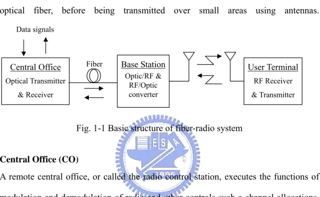
(16) 1.3 Fundamental of RoF 1.3.1 Basic structure RoF uses highly linear optical fiber links to distribute RF signals from a central location to base station (BS), as indicated in Fig. 1-1. In this architecture, signals are generated at a central office (CO) and then distributed to remote base stations using optical fiber, before being transmitted over small areas using antennas. Data signals. Fiber. Central Office. Base Station Optic/RF & RF/Optic converter. Optical Transmitter & Receiver. User Terminal RF Receiver & Transmitter. Fig. 1-1 Basic structure of fiber-radio system Central Office (CO) A remote central office, or called the radio control station, executes the functions of modulation and demodulation of radio and other controls such a channel allocations. Such concentrated execution of these troublesome functions provides a much simplified and cost-effective radio access network and promises easy realization of recent advance demodulation techniques, such as macro-diversity and handover control. Base Station (BS) The interface receiving or radiating radio signals in each radio zone, call the BS, equips only the converter between radio signals and optical signals. The BS requires neither the modulation functions nor demodulation functions of radio. The radio signals converted optical signals are transferred via a fiber optic link with the benefit of its low transmission loss. Therefore, the architecture of fiber optic radio access links can be independent of the radio signal format and can provide many universal 4.

(17) radio access links that are available to any type of radio signal. This means that such radio access links are very flexible to modification of radio formats or the opening of new radio services. User Terminal (UT) At user terminal, the RF signals can be transmitted or received via antennas or mobile interface and so on. The RoF technology allows the BSs to be extremely simple since they only need to contain optoelectronic conversion devices and amplifiers. Functions such as coding, modulation, multiplexing, and upconversion, can be performed at a central location. A simple BS means small and light enclosures (easier and more flexible costs) and low cost (in terms of equipment cost and maintenance costs). Centralization results in equipment sharing, dynamic resource allocation, and more effective management. All of this adds up to an access technology that makes life easier and cheaper for operators. The reason why RoF is able to shift system complexity away from the antenna is that optical fiber is an excellent low-loss (0.2 dB/km optical loss at 1550nm), high bandwidth (50-THz) transmission medium (Fig. 1-2).. Fig.1-2 Low-loss transmission windows of silica fiber in the wavelength regions near 1300nm and 1500nm, the inset shows schematically multichannel operation in the 1500 nm transmission windows. (Ref. Fiber-Optic Communication Technology) 5.

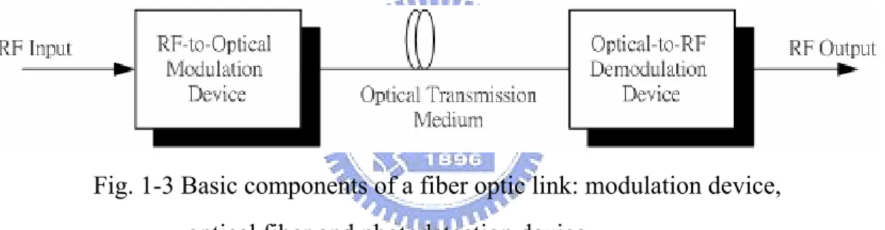
(18) 1.3.2 Optical components Fiber optic radio links employ optical carrier that are intensity modulated by the RF signals and transmitted or distributed to optical receivers via optical fiber. When the modulation of an optical carrier is detected at a receiver, the RF signal is regenerated. Fig. 1-3 illustrates the basic component of a simple fiber optic link. Since the objective of a fiber optic radio link is to reproduce the RF signal at the receiver, the link can convey a wide variety of signal format. In some applications the RF signal is an unmodulated carrier-as for example in the distribution of local oscillator signals in a radar or communication system. In other applications the RF signal consists of a carrier modulated with an analog or digital signal.. Fig. 1-3 Basic components of a fiber optic link: modulation device, optical fiber and photodetection device. Sources of optical signals and the counterpart optical detector are key components of a fiber-radio network. Optical transmitters usually incorporate laser diodes. Transmitter modules generate optical signals at wavelengths according to the operator or standard wavelength specifications. The main requirements from these modules are wavelength stability with time and temperature, ease of control of the laser module, low cost, manufacturability, and reliability. The data to be transmitted is conveyed in the optical signal by modulating the light source directly or external modulator. At the receiver-end, optical networks employ high sensitivity photodetectors together with adequate amplification and electrical processing to provide the best recovery of the transmitted data. 6.

(19) a. Transmitter The role of an optical transmitter is to convert the electrical signal into optical form and to launch the resulting optical into the optical fiber. Fig. 1-4 shows the block diagram of an optical transmitter. It consists of an optical source, a modulator, and a channel coupler. Semiconductor lasers or light-emitting diodes are used as optical sources because of their compatibility with the optical-fiber communication channel. The coupler is typically a microlens that focuses the optical signal onto the entrance plane of an optical fiber with maximum possible efficiency.. Fig. 1-4 Components of an optical transmitter. Semiconductor laser diode and module The development of multi-quantum-well laser(MQW laser)[6-7] cam improve the temperature characteristics, an effect which is due to the reduction of the gain saturation and threshold current density and improvement of optical confinement in the well. As the result, high performance MQW-DFB lasers, which show an ultra-low threshold current, narrow linewidth, high output power, high temperature operation and high reliability, are developed. RF signals transmission using semiconductor laser diodes has attracted much attention. So far, many efforts have been made to improve the characteristics of laser diodes. Generally, semiconductor laser diode is divided into single-mode laser such as the distributed feedback laser diodes (DFB-LDs) and multimode laser such as the 7.

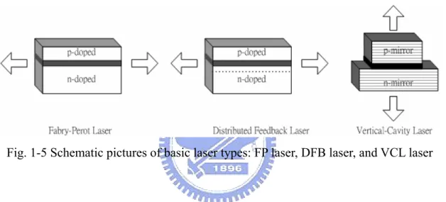
(20) Fabry-Perot laser diodes (FP-LDs), which show a low threshold current, high power output [8-9]. The FP-LDs have a high relative intensity noise (RIN) because of mode competition [10-11]. On the contrary, a DFB-LD oscillates stable even in a wide range of temperature and under high-speed modulation conditions. Modern laser diodes use a sandwich-like structure of different semiconductor materials to form the p-n junction. Fig. 1-5 shows three types of optical cavity designs of laser diodes.. Fig. 1-5 Schematic pictures of basic laser types: FP laser, DFB laser, and VCL laser. The simplest design uses the reflection at the two laser facets to form a Fabry-Perot (FP) resonator in the longitudinal direction. Constructive interference of forward and backward traveling optical waves is restricted to spectrum of the laser. The resonator length is typically in the order of hundred micrometers, much larger than the lasing wavelength, so that many longitudinal modes may exist. The actual lasing modes are given by the quantum well gain spectrum. Single mode lasing is hard to achieve in simple FP structures, especially under modulation. Dynamic single mode operation is required in many applications and it is achieved using optical cavities with selective reflection.. 8.

(21) The distributed feedback (DFB) laser is widely used for single mode applications [11]. Typical DFB lasers employ a periodic longitudinal variation of the refractive index within one layer of the edge-emitting waveguide structure as shown in Fig. 1-5. An emerging low-cost alternative to DFB lasers are vertical-cavity- lasers (VCLs) which emit through the bottom and/or top surface of the layered structure. In VCLs, distance and layer thickness of the two distributed Bragg reflectors (DBRs) control the lasing wavelength (Fig. 1-5) [12]. However, long-wavelength VCLs are still under development and their slope efficiency are relatively low [13-14]. Two types of transmitters have been developed: intensity modulated semiconductor laser and external modulator. The former has the advantages of being simple, compact, and low cost. On the other hand, the external modulator offers high power and low chirp. Therefore, the external modulator is widely used in optical amplified trunk systems that need higher power budgets and super performance [15-16]. Direct modulation The simplest way of converting electrical signals into optical ones is by directly modulating a laser diode. It based on the fact that electrons flowing through the semiconductor diode generate photons. Thus by modulating the current via s modulated microwave/millimeter-wave signal, the intensity of the emitted light will be modulated in the same way. In Fig. 1-6, laser diode characteristic are revealed together with characteristic quantities.. 9.

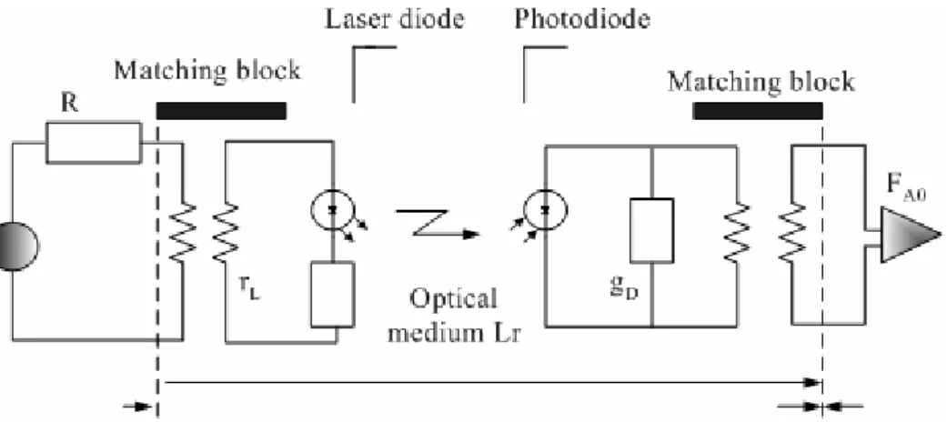
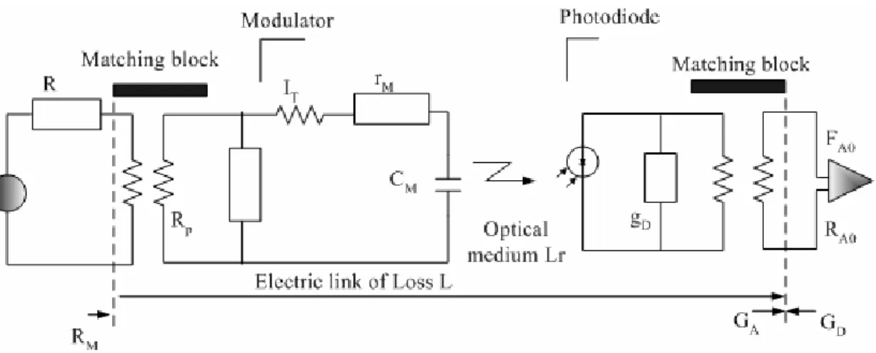
(22) Fig. 1-6 Schematic optical power versus current characteristic of a laser diode. Output optical power versus current can be given as. Popt ( I ) =. hf η L ( I − I th ) e. (1-1). where h is Plank’s constant; f is the optical carrier frequency; e is the charge of the electron; and ηL is the quantum efficiency of the laser diode which is the average number of generated photons per electron. The structure of direct-modulated optical microwave link is shown in Fig. 1-7. The transformers can represent any lossless matching circuit. Of course, practical transforming networks are not lossless; it is tacitly assumed that rL and gD include losses of these matching networks.. Fig. 1-7 Direct-modulated optical microwave link 10.

(23) Direct modulation of semiconductor lasers is simpler to implement than external modulation. Hence it is the most commonly used method to achieve intensity modulation of the optical carrier, primarily because it is less expensive. However, there are a few reasons that could rule out its application. The first one is bandwidth: The useful bandwidth of modulation is limited to the range from DC to the laser relaxation resonance. Although lasers with modulation cutoff frequencies up to about 40 GHz were reported [17], commercially available laser diodes usually have cutoff frequencies of a few tens of GHz. Further, it can be show that a change in the laser current also results in a change in the optical frequency [18]. This chirping phenomenon results in frequency modulation superimposed on the (wanted) intensity modulation. This may or may not harmful. However, fields modulated by an external modulator are virtually free from chirping. A third advantage of the external modulator over direct modulation could be the higher achievable gain. Gain of an externally modulated link can be increased by increasing the optical power. External modulation. External optical modulator functioning is based on at least three different principles: electro-optical, electroabsorption, and interferometric modulators. The modulator based on a Mach-Zehnder interferometer is the most widely applied. A simplified diagram of a Mach-Zehnder interferometer is shown in Fig. 1-8.. Fig. 1-8 Schematic representation of a Mach-Zehnder modulator 11.

(24) Light is propagating in a plane optical waveguide realized on a substrate mode of an electro-optic material (usually a lithiumniobate), the refraction index of which is controllable by an applied electric field. At cross section A the input optical field is divided into two halves. If the modulating signal is applied on the electrodes, the phase shift of the optical field in the upper branch of the structure will varying according to the temporal variation of the signal, while that of the lower branch will remain constant. At cross section B the two optical field interfere with each other, resulting in a modulated amplitude and consequently in a modulated intensity. The design shown in Fig. 1-8 is the simplest one. Applying different and more complex structures for electrodes having various special characteristic can be achieved: push-pull operation, single-sideband modulation, and others [19-21]. From electrical point of view, the modulator electrodes are regarded basically as a capacitor. This can be lossy and a parallel matching resistance can be applied. Further, a series inductor can be applied in order to tune the capacitor to resonance. Thus, the general electrical block schematic of an optical link with a Mach-Zehnder modulator is shown in Fig. 1-9, and in this figure, the “optical medium” and the receiver part are the same as those shown for the direct modulated link in Fig. 1-7.. Fig. 1-9 External modulated optical link: It, tuning inductor; rM, CM, resistance and capacitance of the modulator electrodes, respectively; and Rp, possible matching resistor. 12.

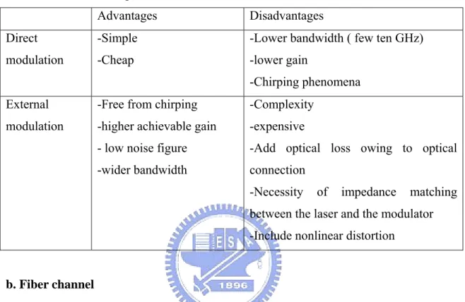
(25) Table 1-1 gives a summary of the advantages and the disadvantages of the direct modulation and the external modulation.. Table 1-1 Comparisons of direct modulation and external modulation Advantages. Disadvantages. Direct. -Simple. -Lower bandwidth ( few ten GHz). modulation. -Cheap. -lower gain -Chirping phenomena. External. -Free from chirping. -Complexity. modulation. -higher achievable gain. -expensive. - low noise figure. -Add optical loss owing to optical. -wider bandwidth. connection -Necessity. of. impedance. matching. between the laser and the modulator -Include nonlinear distortion. b. Fiber channel. The role of communication channel is to transport the optical signal from transmitter to receiver without distorting it. Most lightwave systems use optical fibers as the communication channel because fibers can transmit light with a relatively small amount of power loss. The optical fiber is the transparent flexible filament that guides light from a transmitter to a receiver. The input RF signal is applied to a laser diode where it modulates the intensity of the output light. In most cases this light will have a wavelength of either 1300 or 1550 nm for low transmission loss in silica fiber. The fiber may be multimode or single mode, although the latter is preferred for link spans of more than a few tens of meters for its low dispersion properties, as shown in Fig. 1-10. And Table 1-2 provides a quick reference guide to cable parameters.. 13.

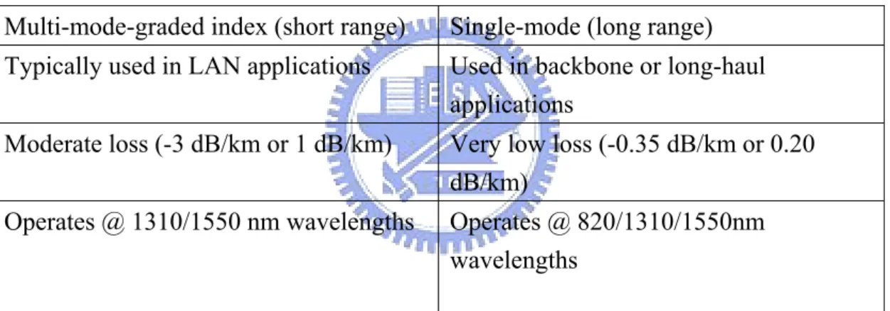
(26) Fig. 1-10 Typical spectral attenuation curves of single mode and multimode fibers. (Ref. Djafar K. Mynbaev and Lowell L. Scheiner,Fiber-Optic Communication Technology, 2001) Table 1-2: Cable parameters Multi-mode-graded index (short range). Single-mode (long range). Typically used in LAN applications. Used in backbone or long-haul applications. Moderate loss (-3 dB/km or 1 dB/km). Very low loss (-0.35 dB/km or 0.20 dB/km). Operates @ 1310/1550 nm wavelengths. Operates @ 820/1310/1550nm wavelengths. (Ref. John C. Bellamy, .Digital Telephony, 3rd edition, 2000). c. Receiver. An optical receiver converts the optical signal received at the output end of the optical fiber back into the original electrical signal. The key component of an optical receiver is its photodetector. The major function of a photodetector is to convert an optical information signal back into an electrical signal (photocurrent). The optical detector plays an important role in an analog fiber link as its performance determines the baseline characteristics of the link.. 14.

(27) Fig. 1-11 Components of an optical receiver. The responsivity Rp of a detector is the ratio of the output electrical response to the input optical power and can be expressed as R p = Mη. e A /W hν. (1-2). in which η is the external quantum efficiency, it is defined as the ratio of the number of electrons generated to the number of incident photons before any photogain occurs, Photogain M can result from carrier injection in semiconductor materials, as in the case of photoconductive devices, or from impact ionization, as in the case of an avalanche photodiodes. M is the current multiplication factor of the avalanche photodiode at microwave frequency. In the case of a p-i-n photodetector, M=1. For application where a relatively low level of optical power is incident on the photodetector, the responsivity remains unchanged as the optical power is varied slightly. The relation between R (η) and wavelength is usually referred to as the spectral response characteristic. For fiber-radio systems, the optical receiver usually consists of a p-i-n photodiode, which provides an RF output power which is proportional to the square of the input optical power. This type of optical link is known as intensity modulated-direct detection (IM-DD). Other types of link are possible involving frequency or phase modulation, but for cellar applications the IM-DD links are used for reasons of simplicity and cost. 15.

(28) 1.4 Motivation Current applications of fiber optical communication systems are proceeding in two directions. One is high bit-rate long-haul transmission utilizing long-wavelength light source, high-performance transmission fibers and low-noise broadband optical amplifiers. The other is high capacity, short distance such as local area networks (LANs), FTTA (Fiber to The Area) and FTTH (Fiber to The Home). The FTTH is the ultimate solution for last-mile access networks. These applications are focusing on reducing the cost of network components and deployment rather than pieces of custom designed systems, which will determine the accepted timing of vast end users. Hybrid radio/fiber networks are an attractive option to realize FTTH. With the development of mobile communications, the growing demand for high bandwidth which will permit broadband applications to be delivered to end-users, forces the system operators to seek new ways to increase the bandwidth and capacity of telecommunication systems. Radio over fiber (ROF) technology will play a significant role in realizing broad-band networks. Although the bandwidth demand of broadband services has been tremendously reduced by video compression techniques the existing access network infrastructure represents a bottleneck for these services. As the network evolution should be adapted to the service demand hybrid fiber based architectures offer a high potential as a bridge or even alternative to FTTH. Combining the techniques of radio and fiber systems makes use of both their merits: fiber provides a high capacity medium with electromagnetic interference immunity and low attenuation, while radio solves the problem of “the last mile”: enabling broadband data to be delivered to the end-users in a fast and cost-effective manner. Furthermore, in order to support many base stations, a low-cost transmitter at BS is necessary for the general market acceptance. However, the relative high cost. 16.

(29) of the distributed feedback (DFB) laser or electric absorption modulator (EAM) used to transmit radio signals in the radio access unit (RAU) is hard acceptance of subscribers [22-23]. Therefore it will be required to design a cost-effective structure and fiber-radio interferences. On the basis of injection-locked Fabry-Perot laser diode (FP-LD), the proposed scheme can provide a purely single longitudinal mode and thus greatly reduce the RAU cost. Besides, we also offer a dynamic add-drop wavelength technique by a fiber Bragg grating array (FBGA) in the remote node, which can provide a simple and efficient method to solve the burst transmission load problems.. 1.5 Outline of the thesis In this thesis, the introduction is given in Chapter 1 including history background and fundamentals of RoF technology. In Chapter 2, firstly we surveyed current network technology then we proposed a hybrid fiber-radio network architecture and illustrate the generic characteristics in this network. System simulation and analysis are performed in Chapter 3, such as optical spectrum of injection-locked FP-LD, frequency response, bit error rate measurement and so forth. In Chapter 4, we experimentally verified this architecture. Finally, we conclude the study in Chapter 5.. 17.

(30) Chapter 2 Hybrid Fiber-Radio Network. 2.1 Survey of fiber-radio highway Fiber optic radio access networks are optical backbone networks for radio access systems, where fiber optical links have the function of transferring radio signals into remote stations without destroying their radio format, such as RF, modulation format, and so on. For the purpose, the transmission format in the fiber optical networks is typically based on analog optical modulation techniques [24-30]. The concept of fiber optic radio access networks is illustrated in Fig. 2-1.. Fig. 2-1 Concept of fiber radio networks Consequently, fiber optic radio access networks are considered hopeful candidates for various future cellular radio access networks, such as third generation mobile communication systems, fixed wireless access systems, wireless LAN, roadside-to-vehicle radio access links in intelligent transport systems (ITS), or distribution systems of CATV signals.. 18.

(31) 2.1.1 Network topology Three candidates are under consideration for the link configuration topology in constructing networks: star configuration, ring configuration, and bus configuration. Fig. 2-2 illustrated these three configurations.. Fig. 2-2 Various network configurations The star configuration is the most popular one because of its easy maintenance, high reliability, and simple construction. The most common type of star configuration is the passive double star. However, it is difficult to construct or extend star networks cost effectively or quickly because the same fiber counts are required as the number of RBSs, and it is difficult to increase the number of RBSs when cell splitting is required. However, the bus configuration or the ring configuration can reduce the fiber counts by quite a bit; thus, they offer cost-effective and quick construction of networks and also easy extension of RBSs. These capabilities are very important in constructing fiber optic radio access networks because the density of RBSs increases according to the number of users, and becomes very high in recent microcellular 19.

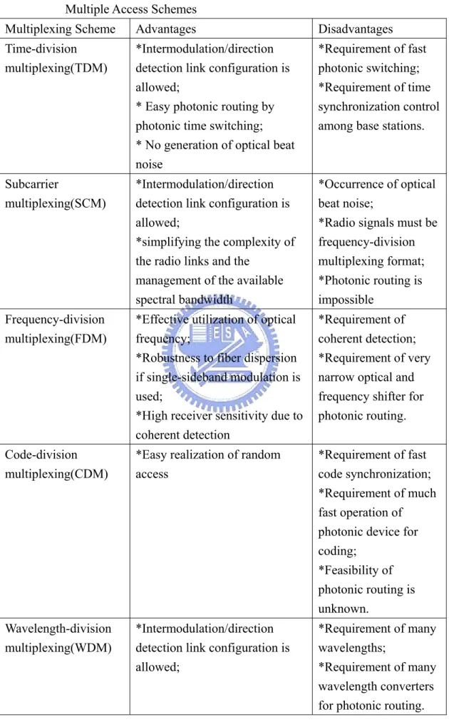
(32) requirements. For indoor use, network flexibility and fiber count reduction are very important matters, because the reinstallation of fiber is wasteful. Therefore, we should study the fiber optic links that use the bus or the ring configuration. These two configurations are quite similar except for the difference of whether the network is terminated at a certain RBS or at the RCS.. 2.1.2 Photonic multiplexing Many subjects must be studies in order to realize fiber optic radio access networks that connect BSs to CSs. One basic subject is which photonic link configuration and multiplexing scheme are suitable for the construction of fiber optic radio access networks. There are various types of link configuration and photonic multiplexing schemes, such as subcarrier multiple access, photonic frequency-division multiple access of WDM access, photonic time-division multiple access, photonic code-division multiple access, and chirp multiplexing transform access and routing. The features of each scheme are summarized in Table 2-1. In discussing which photonic multiplexing scheme is suitable for radio access networks, it needs to make much of the cost efficiency, the ease of use, and the simplicity of network construction because these are the most important benefits offered by fiber optic radio access networks. In selecting a particular photonic multiplexing scheme, it is also important to make much of the feasibility for the routing of radio signals, and it is desirable for the routing process to be executed at the optical stage.. 20.

(33) Table 2-1 Performance Comparison of Advantages and Disadvantages of Various Multiple Access Schemes Multiplexing Scheme. Advantages. Disadvantages. Time-division multiplexing(TDM). *Intermodulation/direction detection link configuration is allowed; * Easy photonic routing by photonic time switching; * No generation of optical beat noise. *Requirement of fast photonic switching; *Requirement of time synchronization control among base stations.. Subcarrier multiplexing(SCM). *Intermodulation/direction detection link configuration is allowed; *simplifying the complexity of the radio links and the management of the available spectral bandwidth. *Occurrence of optical beat noise; *Radio signals must be frequency-division multiplexing format; *Photonic routing is impossible. Frequency-division multiplexing(FDM). *Effective utilization of optical frequency; *Robustness to fiber dispersion if single-sideband modulation is used; *High receiver sensitivity due to coherent detection. *Requirement of coherent detection; *Requirement of very narrow optical and frequency shifter for photonic routing.. Code-division multiplexing(CDM). *Easy realization of random access. *Requirement of fast code synchronization; *Requirement of much fast operation of photonic device for coding; *Feasibility of photonic routing is unknown.. Wavelength-division multiplexing(WDM). *Intermodulation/direction detection link configuration is allowed;. *Requirement of many wavelengths; *Requirement of many wavelength converters for photonic routing.. 21.

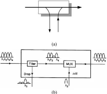
(34) 2.2 Proposed fiber-radio architecture Fig. 2-3 illustrates the proposed fiber-radio architecture that is capable of providing individual customer access to broadband services. At the central office (CO), multiple WDM channels and the corresponding RF carriers are multiplexed together using an optical multiplexer to the remote node (RN) via an optical fiber network. At the RN, the WDM channels are demutiplexed using an optical add-drop multiplexer (OADM) before being routed to the designated RAU. In the upstream path, multiple WDM channels are likewise received from the RAUs before they are multiplexed at the RN via an OADM and transported over the optical fiber network back to the CO.. OMUX: Optical multiplexer ODMUX: Optical demultiplexer OADM: Optical Add/Drop Multiplexer PIN-PD: p-i-n photodetector PC: Polarization Controller Amp: Electrical Amplifier Fig. 2-3 Hybrid Fiber-Radio Network. 22.

(35) Within this architecture, sub-carrier multiplexing (SCM) is used for simplifying the complexity of the radio links and the management of the available spectral bandwidth [31]. In addition to SCM, this hybrid radio/fiber distribution networks employ wavelength division multiplexing (WDM) and optical add-drop multiplexing (OADM) to allow different base-stations to be fed with a common fiber. And then these techniques can simplify the network architecture and improve the deployment of the BS [32]–[36]. But the relative high cost of the transmitters with distinct wavelength has restrained the general market acceptance. Therefore, we use the same wavelength in the upstream from downstream light with low-cost injection-locked FP-LD. OADM. The schematic diagram of an OADM is presented in Fig. 2-4. The optical add/drop multiplexer (OADM) is a unit that selectively removes one wavelength λi from a multiplicity of wavelengths λ1,…, λi, …,λN, multiplexed on an incoming fiber, bypass all other wavelengths, and adds the same wavelength generally with another data content on the transmission fiber (Fig. 2-4(a)).. (a). (b) Fig. 2-4 (a) OADM principle (b) a simple example of a static OADM 23.

(36) An optical add/drop multiplexer (OADM) is an optical component that is used to modify the flow of traffic through a fiber at a routing node. An OADM passes traffic on certain wavelengths through without interruption or opto-electronic conversions, which other wavelengths are added or dropped, carrying traffic originating or terminating at the node. Transmission path (downlink). For the downstream case, the RF signal is used to directly modulate the output of distributed feedback laser diode (DFB-LD). After the downstream wavelength is dropped at the RN, we employ the light injection-locked scheme to remodulate a Fabry-Perot laser diode (FP-LD) at RAU for carrying upstream data traffic. Fig. 2-5 demonstrates the concept of light injection mode-locked. The downstream light channel is split into two parts by a 1×2 coupler and an optical circulator is used to separate the reflected and injection-locked upstream signal from the downstream data.. upstream to central office. RAU. Up link 1×2coupler. circulator. FP-LD. upstream traffic. DFB-LD. FP-LD. Down link. downstream traffic downstream form central office. Fig. 2-5 Operation principle of injection mode-locked of FP-LD. Thus the downstream light beam has two folds of usage: conveying downstream data and light injection-locked to the FP-LD. With injection-locked, the FP-LD exhibits a high SMSR which would not only reduce mode partition noise but also alleviate fiber dispersion. 24.

(37) Received path (uplink). We reuse the same wavelength in the upstream data traffic from the downstream light beam after light injection-locked at the RAU. Then the remodulated upstream channel is inserted to WDM channels at RN and received at the central office.. 2.3 Mathematic model of injection mode-locked FP-LD A mathematic model was designed to simulate the system and to verify the results obtained. It used the laser rate equation to describe the operation of the laser. There are many different forms of the laser rate equations and almost every work undertaken uses a slightly different form. The form we used for our free running laser was very similar to those used before normalization by Le Bihan and Yabre [37]. In [38], Yabre neglects the gain compression factor, ε, by assuming that the optical power is moderate enough to allow the approximation ( εS << 1) and hence (1- εS )≈ 1. For simplification purposes, we used this approximation in our model as the optical power levels in our work are moderate. For the injection-locked case, we added the final term in Eq. (2-2) and the final term in Eq. (2-3) [39]. These terms describe the level and the phase of the injected light. The single mode rate equations for injection-locked laser with photon density S(t), corresponding phase φ(t) and carrier density N(t) used in the model are as. follows: dN (t ) I (t ) N (t ) = − − g 0 ( N (t ) − N om ) S (t ) τn dt qV. (2-1). dS (t ) S (t ) N (t ) = Γg 0 ( N (t ) − N om ) S (t ) − + Γβ + 2 K c S inj S (t ) cos(φ (t )) dt τp τn. (2-2). dφ (t ) α ⎛⎜ 1 = Γg 0 ( N (t ) − N om ) − ⎜ dt 2⎝ τp. (2-3). ⎞ S inj ⎟ − ∆ω − K c sin(φ (t )) ⎟ S (t ) ⎠. 25.

(38) Table 2-2 Parameters in mathematic model g0(m-3s-1) -3. Gain coefficient. Nom(m ). Transparency carrier density. V(m3) τp(s). Volume of the active region. τn(s). Carrier lifetime. Γ. Optical confinement. β. Spontaneous emission factor. q(C) α. Electron charge. I(t) (mA) Δω. Injection current. Photon lifetime. Linewidth enhancement factor. -3. Sinj(m ) -1. Kc(s ). Detuning frequency Photon density of the injected light Coupling coefficient for the injected light. The first step in the design of the full system model was the characterization of the intensity modulation response of the laser diode. Small signal analysis was used. In small signal analysis, time varying components are considered to have a dc part and an ac part. The following were substituted into Eq.(2-1)-(2-3) I (t ) = I 0 + δI , S (t ) = S 0 + δS ,. (2-4). N (t ) = N 0 + δN ,. φ (t ) = φ 0 + δφ , where I0, S0, N0, φ0 are the dc parts, and δI, δS, δN, δφ are the ac parts of the current, photon density, carrier density and phase, respectively. Ignoring the steady state solution and higher order terms yields a set of linearized equations for the ac components of S(t), N(t) and φ(t). 26.

(39) ⎛ jω + a11 ⎜ ⎜ a 21 ⎜a ⎝ 31. a12. a13. jω + a 22. a 23. a32. jω + a33. ⎞ ⎟ ⎟ ⎟ ⎠. ⎛ δN ⎞ ⎛ δI / qV ⎞ ⎜ ⎟ ⎜ ⎟ ⎜ δS ⎟ = ⎜ 0 ⎟ ⎜ δφ ⎟ ⎜ 0 ⎟ ⎝ ⎠ ⎝ ⎠. (2-5). where a11 =. 1. τn. + g 0 S 0 , a12 =. a 21 = −Γg 0 S 0 a31 = −. α 2. Γg 0. 1. τp. −. X , a13 = 0 ΓS 0. ,. a 22 =. X 2S 0. , a 22 = 2S 0Y. ,. a32 =. −Y 2S 0. , a33 =. X 2S 0. and. X = 2 K c S inj S 0 cos(φ 0 ) , Y = K c. S inj S0. sin(φ 0 ). The modulation response was taken as δS/δI. I0 is a known constant which represents the bias current. The dc values of photon density, current density and phase can be obtained by letting the left-hand side of Eqs. (2-1)-(2-3) above equal zero. Using the relationship, cos2A+sin2A=1, and adding manipulated versions of 2 and 3, yields the following: Kc. 2. S inj S0. 1 ⎡⎛ 1 = ⎢⎜ Γg 0 ( N 0 − N om ) − ⎜ 4 ⎣⎢⎝ τp. 2. ⎡α ⎛ ⎞ Γβ N 0 ⎤ 1 ⎟+ + ⎢ ⎜ Γg 0 ( N 0 − N om ) − ⎥ ⎜ ⎟ Sτ ⎥ τp ⎢⎣ 2 ⎝ 0 n ⎦ ⎠. ⎤ ⎞ ⎟ − ∆ω ⎥ ⎟ ⎠ ⎦⎥. 2. (2-6) Letting the left-hand side of Eq. (2-1) equal zero and rearranging gives: I0 N0 − qV τ n = S0 g 0 ( N 0 − N om ). (2-7). Substituting for S0 in Eq. (2-6) yields a quartic equation in N0 that Matlab can easily solve, giving the dc value for carrier density. From this S0 can then be obtained using Eq. (2-7) and φ0 can be obtained form Eq. (2-2) or (2-3). Once these are obtained, then every value in the equation is known and hence the modulation response can be obtained. 27.

(40) 2.4 Generic transmission characteristics 2.4.1 Noise characteristics There are three dominant noise sources in photonic links: relatively intensity, thermal, and shot noise. Dark current noise is negligible, compare to other ones; thus, it can be neglected. All noise sources are statically independent, so the total noise power from all these sources is simply the sum of the independent noise powers. Fig. 2-6 illustrates the equivlent circuit of the PIN direct receiver.. Fig. 2-6 Receiver equivalent circuit with signal and noise current sources. Relative intensity noise (RIN) of the laser diode. The light laser diodes with the quantum nature are intrinsically relatively noisy devices. Thus relative intensity noise is a quantization noise due to the light being quantized into energy packets (i.e. photons), which is influenced by temperature, bias voltage, laser structure, and other factors that effect the laser output power [39]. The main noise source in laser diodes is represented by the spontaneous emission noise, yielding fluctuations of the emitted optical intensity and the emission frequency. These fluctuations are known as the relative intensity noise (rin) which is defined as rin =. < δP 2 > ∆f 2. (2-8). Relatively intensity noise of laser is usually specified in terms of RIN. RIN related to rin by RIN = 10 log10 rin. (2-9) 28.

(41) Both the <δP2> and 2 the will produce corresponding currents squared in the load resistor after detection. The same detector and circuit will be used for <δP2> and 2, the ratio of <δP2>/2 is the same as <irin2>/<ID>2, where ID is the average received photocurrent. Hence the relative intensity noise within a filter bandwidth Be can be represented as a current generator with a mean square current as 2. < irin >= rin 2 Be. (2-10). The RIN spectrum is not flat and hence this is not a white noise source. However, for simplicity, most link analyses assume that RIN is a constant within the bandwidth of interest. RIN also differs for diode and solid state lasers, and for single mode and multimode lasers. This can observed in a weak signal and also includes the spontaneous emission to the coherent light of the laser output. To measure the RIN the optical power is converted to a current after the receiving photodiode and the noise of this photocurrent may be easily measured with an RF spectrum analyzer. A typical plot of RIN is shown in Fig. 2-7. The peak of the RIN curve coincides approximately with the relaxation oscillation frequency of the laser.. Fig. 2-7 RIN versus frequency at a few optical power levels (Ref. Hamed Al-Raweshidy Shozo Komaki, Radio over Fiber Technologies for Mobile Communications Networks, 2001) 29.

(42) Shot noise within the photodetector. Shot noise is generated whenever an electrical current with average value is generated via a series of independent random event, e.g. the photocurrent in a detector. Shot noise is a white noise source and the generation of charge carriers is characterized by Poisson statistics. The shot noise is represented by a mean square shot noise current generator, 2. = 2e Be. (2-11). Because the shot noise is linearly proportional to ID, the shot noise can be larger than the thermal noise for sufficiently large ID. It is one of the disadvantages of using high input laser power. Thermal noise at the receiver. Whenever any resistor is used in a circuit, it generates thermal noise, which is also known as the Johnson noise. Thermal noise is a white Gaussian noise caused by radiation from random motion of electrons. To limit the noise power contributed by such a broadband noise source, there is usually an electrical filter of bandwidth Be put in the circuit. Only the signals and the noise within this band need to be considered in the link. The thermal noise is commonly treated as a mean square current noise generator in parallel with a noise-free resistor R. The mean square noise current of the thermal noise is 2. < ith >=. 4kTBe R. (2-12). Thermal noise exists even if there is no incident optical power at the receiver.. 30.

(43) 2.4.2 Distortion characteristics Harmonic distortion. A sinusoidal current modulation generates light power modulations at the input frequency ω and also at the harmonics 2ω, 3ω,…, nω. The amplitude of the nth order harmonic is proportional to the nth power of the optical modulation index (OMI) and it decreases rapidly with higher order. Harmonic distortion depends on the nonlinearity of a transmission system. In the case of laser diodes, it is related to the nonlinearity of the L-I characteristic. Intrinsic distortion. Even with perfectly linear L-I characteristics, distortions are generated by the intrinsic interaction of electrons and photons during stimulated recombination. Intrinsic distortion dominates at frequencies near the resonance frequency fr and often limit the useable bandwidth to low frequencies f << fr. At low frequencies, the distortion is governed by the nonlinearity of the L-I curve of the laser diodes (static distortion). Intermodulation distortion. Intermodulation distortion arises when two or more signals at different modulation frequencies are transmitted. Two signals at ω1 andω2, for example, are accompanied by second order distortions at frequencies 2ω1,2 , ω1±ω2, and , third order distortions at frequencies 3ω1,2 , 2ω1±ω2, and 2ω2±ω1,etc. The third order modulation distortions (IMDs) at 2ω1-ω2 and 2ω2-ω1 are special interest since they are close to original signals and they might interfere with other signals in multichannel applications. The third order IMD increases as the cube of the OMI [40]. The amplitudes of intermodulation distortions can be related to the amplitudes of harmonic distortions (those relations depend on the dominating cause of the distortion: intrinsic or static distortion). In multichannel applications, distortions from several channels add up and they 31.

(44) are described by composite second order (CSO) and composite triple beat (CTB) quantities. Additional distortions from clipping occur when the combined OMI of all channels is larger than one, i.e., when the total modulation current drops below the threshold current [19]. Fig. 2-8 gives a plot of the distortion characteristics versus modulation frequency.. Fig. 2-8 Distortions vs. modulation frequency (Ref. William S.C. Chang, RF Photonic Technology in Optical Fiber Links 2002). 2.4.3 Carrier to noise ratio (CNR) An RF lightwave system consists of transmitters, fiber link, and receivers. The performance of this kind of system in then determined by the performance of those active and also passive components, such as the effect of fiber link “stimulated” by the light. All these can be quantified by carrier-to-noise-ratio (CNR), and second and third order distortions (CSO and CTB), which directly determine the received signal quality at the customer premises equipment (e.g., TV set). This is shown in Fig. 2-9. 32.

(45) Fig. 2-9 CNR, CTB, CSO in RF subcarrier system. (Ref. William S.C. Chang, RF Photonic Technology in Optical Fiber Links 2002). Excluding fiber effects, the received CNR after optical fiber transmission, is given as 2. CNR =. ID =. 2. 2. + < ith > + < irin. 2. 1 (mI D ) 2 2 = > B (2eI + 4kT + rin × I 2 ) e D D R. ηe PD = R p PD hν. (2-13). (2-14). Optical modulation index (OMI) m is defined as. m=. ∆I ∆P = ^ I b − I th P. (2-15). An improved signal/noise ratio is obtained with increasing optical modulation index (OMI) m. However, the upper possible m is limited by nonlinear distortion. Thus to avoid overmodulation of a light source, we make sure that 0 ≤ m ≤ 1.. 33.

(46) Table 2-3 Parameters used in CNR calculation e. electron charge. h. Plank’s constant. k η. Boltzmann’s constant quantum efficency of the photodiode. ν. optical carrier frequency. T. Temperature in kelvin. Be. noise bandwidth per channel. m ΔI. optical modulation index (OMI) per channel The variation of electrical driving current around a bias point in modulating a laser light source. Ib. The laser bias current. Ith. The laser threshold current which the light source starts to emit coherent light. ID. average received photocurrent. PD. average received optical power. Rp(A/W). Responsivity of the photodiode. R. noise-free resistor 2. (mI0) /2. signal power per channel. 2BeeID. shot noise. Be(4kT/R). thermal noise of the receiver. rin. relative intensity noise of the laser diode. From Eqs. (2-13)-(2-15), one can determine the necessary optical power to achieve the desired CNR.. 2.4.4 Summary Two approaches could improve system performance. First, increasing optical power would improve CNR performance. Second, driving the laser harder would also improve CNR performance but degrade the CTB and CSO. Further, when driving the laser too hard, the electrical signal may drive the laser below the threshold current, which makes the output optical signal chirp, and creates broadband distortion [41-44]. 34.

(47) The distortion is a function of the root-mean-square (RMS) modulation depth of the total signal, u = m N / 2 . Optimizing system performance is then a question of balancing the OMD, optical power, and other related issues. From Eq. (2-13), the shot noise and laser’s RIN dominate the CNR performance with high received optical power. While lower received power, the receiver thermal noise become significant. In that situation, the link performance can improve by reducing this noise. This can be achieved by improving the impedance match between the photodiode, which is an infinite-impedance current source, and the low-noise amplifier. Nevertheless, this approach leads to two limitations. First, the RC circuit to accomplish the impedance match imposes a bandwidth limitation. Second, the increased impedance increases the signal level that requires much more linear preamplifier. Consequently, in an RF lightwave system, transmitter, receiver and optical fiber will contribute to the CNR, CTB, and CSO performance in many different ways. The system (end-to-end) performance is then a balance among those variables.. 35.

(48) Chapter 3 System Simulation of Hybrid Fiber-Radio Network In this chapter, we simulate the proposed hybrid fiber-radio network. First, we observe characteristics of the laser diodes, especially for injection mode-locked FP-LD. Then, we simulate system performances including bit-error-rate measurement and eye pattern measurement. Finally, we numerically estimate carrier-to-noise and distortion ratio for many base stations.. 3.1 Software interpretation The hybrid fiber-radio network presented in Chapter 2 has been simulated using the Virtual Photonic Inc. (VPI) Transmission Maker software package. It is a comprehensive tool and excellent simulation environment for characterization and designs of devices or systems. It is used to analyze new concepts, optimize designs and evaluate new devices and their impact on subsystems. Moreover, it can also support verification of component designs in terms of their overall effect on system performance.. 3.2 Injection-locked of FP-LD The injection-locked scheme has been mentioned previous. In this section, we show the simulate results of FP-LD with and without injection-locked, including optical spectral, the relation of injection power and output power, frequency response of modulation, and RF spectra of RF carriers.. 36.

(49) 3.2.1 Optical spectra Fig. 3-1 shows the optical spectra of FP-LD under the condition of free-running and injection-locked. The mode spacing of FP-LD simulated is 0.8nm and the central wavelength is around 1550nm. The free-running FP-LD performs multimode operation as shown in Fig. 3-1(a). On the contrary, the injection-locked FP-LD provide superior singlemode light source as evidenced in Fig. 3-1(b). As Fig. 3-1 indicated, the side-mode suppression ratio (SMSR) of the FP-LD was improved from 5.6dB to 45 dB with an injection power of -5 dBm.. (a). (b) Fig. 3-1 Optical spectra of FP-LD (a) free-running (b) injection-locked 37.

(50) The injection-locked FP-LD offers singlemode operation and the improvement in SMSR alleviated the fiber-dispersion-included power penalty on the upstream transmission, thus enhancing the network transmission span. Furthermore, various wavelength of injection-locked FP-LD can be obtained by detuning the central wavelength and bias current of DFB-LD and FP-LD for the purpose of WDM network as displayed in Fig. 3-2.. Fig. 3-2 Various wavelengths of injection-locked FP-LD. 38.

(51) 3.2.2 Relation between injection power and output power In order to investigate the injection mode-locked characteristics in detail, we use an optical attenuator to control the injection power to estimate the relationship between injection power and output power of injection-locked FP-LD. Table 3-1 shows the results of simulation and Fig. 3-3 displays the optical spectra under different injection power.. Table 3-1 Relation between injection power and output power Average power. Main mode of laser diode. Injected power(mW). Out put power(mW). Injected power(dBm). Out put power(dBm). 5.4159. 3.0135. 4.46188. 2.00478. 3.0456. 2.5953. 1.96188. 1.42338. 1.7127. 2.3039. -0.53812. 0.96378. 0.963. 2.0899. -3.03812. 0.59152. 0.542. 1.929. -5.53812. 0.28678. 0.305. 1.8064. -8.03812. 0.03356. 0.171. 1.7122. -10.53812. -0.18642. 0.0963. 1.6448. -13.03812. -0.43335. 0.0542. 1.6048. -15.53812. -1.12326. 0.0305. 1.5533. -18.03812. -2.03141. 0.0171. 1.5155. -20.53812. -3.22383. 0.0096. 1.1111. -23.03812. -7.87846. 0.0054. 1.1066. -25.53812. -11.79314. free-run. 1.0953. free-run. -14.3779. 39. (a). (b). (c). (d).

(52) (a). (b). (c). (d). Fig. 3-3 Optical Spectra of injection-locked FP-LD with different injected power. Table 3-1 reveals that output power of injection-locked FP-LD is proportional to injected input power and the SMSR is a function of the injection power. If the injection power is large enough, the injection-locked FP-LD will perform as a good singelmode light source. However, when the injection power is below -15.538 dBm, the linewidth of the injection-locked FP-LD becomes broadening, as shown in Fig. 3-3(c). And as injection power less than -25.538dBm, the injection-locked FP-LD operate as multimode similar to free-running FP-LD, as given in Fig. 3-3(d). In this simulation, the minimum injection power is -13.038 dBm for SMSR ≧ 20dB. To be clear about the connection between injection power and output power of injection-locked FP-LD, the data of Table 3-1 is diagrammed in Fig. 3-4.. 40.

(53) (a). (b) Fig. 3-4 Plots of output power of injection-locked FP-LD against injection DFB power (a) average power measured by power meter (b) main mode power norm observed by optical spectrum analyzer. 3.2.3 Characteristics of injection FP-LD There are two characteristics of the laser diode that will affect the performance of a fiber-radio system, the magnitude of the response and the linearity of the response. Firstly consider the magnitude of the modulation response of the laser diode. As the magnitude of the laser response increases, then for a given power in the RF signal 41.

(54) driving the laser, the detected electrical signal power will increase. Thus by using the injection-locked to enhance the response of the laser at frequency bands beyond the free-running device, it will clearly result in a major improvement in the performance of the hybrid radio/fiber system [45-46]. The second important characteristic is the linearity of the response at the frequency of interest. If we are operating in a linear portion of the modulation response, the IMD is kept to a minimum. However as the operating RF band approaches the relaxation frequency of the laser, the response becomes quite nonlinear, which will affect the performance of a multi-carrier fiber-radio system. Since the relaxation frequency of DFB-LD is far away from the RF frequency in use (about 6GHz) and FP-LD is opposite (about 1-2 GHz), we focus the nonlinearity problem on FP-LD. To overcome this problem it is possible to make the laser’s response more linear around the relaxation frequency of the free-running device [47-48]. Thus we analyze and compare the characteristics of free-running FP-LD and injection-locked FP-LD. a. RIN Measurement. The setup of RIN measurement is shown in Fig. 3-5. The RIN characterization uses an optical amplifier with defined output power (1 W), to convert an intensity noise spectrum into a relative intensity noise spectrum. The electrical amplifier calibrates the RFSA reading to dB/Hz for the default spectral resolution.. 1550nm. RFSA. PIN-PD. LD. Optical Amplifier NF 4 dB. Electrical Amplifier 10 dB. RF spectrum analyzer. Fig. 3-5 Setup of RIN measurement. 42.

(55) (a). (b). (c) Fig. 3-6 RIN of different types of laser diodes (a) DFB-LD (b) free-running FP-LD(c) injection-locked FP-LD Fig. 3-6 shows the RIN characteristic of DFB-LD, free-running FP-LD, and injection-locked FP-LD. These show that how the RIN of a laser can be determined as 43.

(56) a function of frequency. In Fig. 3-6 we can find that the relaxation frequencies of DFB-LD, free-running FP-LD, and injection-locked FP-LD are near 6, 1.5, and 5.5 GHz, respectively. And the RINs corresponding to these laser diodes at the frequency band in use at this fiber-radio network are approximately -150, -130, and -140 dB/Hz. A low RIN is critical in high-speed and analog systems. This is usually achieved by increasing the output power of the laser. However, make use of high optical power may causing another impairments of the system such as shot noise, distortion due to nonlinearity of the laser diode. We will analyze these characteristics in section 3-5. b. Modulation response. Because of the direct modulation of a laser is limited in frequency by the inherent bandwidth of a laser diode. Publications [49-50] have shown that by using light injection we can improve the modulation bandwidth of a laser. Thus, in this section, we inspect the influence of injection-locking on FP-LD modulation bandwidth. The simulation model of modulation response is given in Fig. 3-7. PIN-PD 1550nm. 1. 3. DFB-LD 1550nm. Amp 10 dB. 2. FP-LD. RF signal. Network Analyzer. Fig. 3-7 Modulation response measurement By varying the frequency of RF signals, we can obtain the frequency response of FP-LD via RF spectrum analyzer. Fig. 3-8(a) shows the modulation response of the FP-LD under free-running condition with different driver dc bias. Fig. 3-8(b) shows the modulation response of the FP-LD without injection and under three different levels of DFB-LD injection. 44.

(57) (a). (b) Fig. 3-8 Frequency Responses of FP-LD (a) Free-running with different dc bias (b) Injection-locked with various injection powers In view of modulation bandwidth, in Fig. 3-8(a), it can be seen that the modulation bandwidth is extending with dc bias of FP-LD increasing; however, the impact on extending the modulation bandwidth is limited (increment less than 1GHz). On the contrary, the modulation bandwidth extends greatly due to injection-locked as shown in Fig. 3-8(b). In addition to modulation bandwidth, the magnitude of RF signal is in the same way. Take RF frequency at 2.9 GHz for example, the gain. 45.

(58) increase more than 10 dB due to injection-locking and only few dB due to increasing dc bias of FP-LD.. 3.2.4 RF Spectra of received RF signals When using multi-channel RF data signals in this work, there are two types of intermodulation products generated that cause interference and degrade the overall performance of SCM system. There are intermodulation of the type 2fi-fj, and also those due to beating between three frequencies fi+fj-fk as previous referred. To overcome the problems caused by these intermodulation products we subsequently use the injection-locked technique. Fig. 3-9(a) shows the electrical spectrum of 3-channel RF data signals that are used to directly modulate the FP-LD, and Fig. 3-9 (b) displays the received electrical spectrum of direct modulated free-running FP-LD after passing through the optical link and being detected with the 10 GHz PIN photodiode. As we can see from this figure, the dynamic nonlinearity of the laser diode around the operating frequency of 2.1-2.5 GHz results in the generation of sideband around the received signal due to IMD. In addition to the sidebands that are visible in the received spectrum, there are also IMD products sitting on the received data channels that will affect the performance of these channels. In the case of injection-locked, the received electrical spectrum is shown in Fig. 3-9 (c). The level of IMD reduces about 2.9dB (from -46.2dBm to -49.1dBm in worst case) and the improvement in the magnitude of RF carriers is 4.1 dB (from -32.6dBm to -28dBm in worst case). It is clear from this result that improved linearity of the FP-LD, around the operating frequency band, greatly reduces the level of IMD and the magnitude of received RF carriers are also enhanced by injection-locked scheme.. 46.

(59) (a). (b). (c) Fig. 3-9 RF Spectra showing (a) the signal which modulated the FP-LD (b) the received signals without injection-locked and showing the IMD effects of laser nonlinearity, and (c) the received signals with injection, showing the reduction in IMD due to increase linearity. 47.

(60) 3.3 Bit-error-rate and eye pattern measurement In section 3.2, those spectra of received RF signals clearly show us that nonlinearity in the free-running FP-LD is introducing signal distortion that can be significantly reduced using injection mode-locked scheme. To determine how the improvement in linearity affects the performance of the overall system it was necessary to measure the bit error rate (BER) of the received signal. In this work, the relative responses of the FP-LD around the operating frequency band with and without injection is the same, thus the improvement in system performance is solely due to the reduction in nonlinearity of the device having decreased the IMD. Fig. 3-10 demonstrates the setup of BER measurement for three RF data channels, for simplicity, on one particular wavelength channel. At the CO, a DFB-LD at 1550 nm is directly modulated with RF signals which is generated by mixing three distinct 100 Mbit/s NRZ 231-1 pseudorandom bit stream (PRBS) data with three RF carriers (2.7, 2.9 and 3.1 GHz) to form the downstream signals, which was then transmitted over a fiber span of 7 km to the RAU. At the RAU, 50% of the downstream signals are tapped off for downstream data reception via a 10 GHz optical receiver while the rest of the signal power (at -5 dBm) is injected into a FP-LD, which is simultaneous directly-modulated with another RF signals which are also generated by mixing three distinct 100 Mbit/s NRZ 231-1 PRBS data with three RF carriers (2.1, 2.3 and 2.5 GHz) to form the upstream signals. The upstream signals are then transmitted over another 7 km fiber span and are received at the central office. To determine the improvement in system performance, an optical attenuator is used to vary the received power and bit error rate is measured as a function of received power.. 48.

(61) Amp. BPF. ASK. Attenuator. PIN-PD. 10dB. SMF 5km Optical Filter. 100Mbit/s NRZ PRBS 231-1 data. Up link SMF 5km. 2.7G. 1x2 coupler. 1550nm. ASK. 2.9G. ∑. DFB-LD. 2.1G. SMF 2km. FP-LD. 3.1G. ∑. Down link. 2.5G. BPF Attenuator. 2.3G. ASK. 100Mbit/s NRZ PRBS 231-1 data. Amp ASK. PIN-PD. 10dB. Fig. 3-10 Simulate setup of BER Measurement Fig. 3-11 shows the plot of the simulated BER against received powers for the overall system of the downstream signal and the upstream signal, measured at BS and CO, respectively. The received optical powers for error-free (10-9) are -13.3dBm, -12.4 dBm, and -10dBm for downstream, upstream with injection-locked, and upstream without injection-locked, respectively. It shows that around 2.4dB improvement was achieved for a received BER of 10-9 when injection-locked scheme is applied to the FP-LD and the power penalty of downstream and upstream in this network is around 0.9dB.. 49.

(62) Fig. 3-11 BER performances of downstream and upstream traffic data1: BER of downstream data2: BER of upstream (injection-locked FP) data3: BER of upstream (free-running FP). Fig. 3-12 shows the simulated eye diagrams of the received 100Mbit/s data signals for downstream and upstream traffic and both measurements show error-free operation and prove the effectiveness of our purposed scheme. Fig. 3-12 (a) displays the case of downstream and Fig. 3-11(b) and (c) is the cases upstream with and without injection-locked into the directly modulated transmitter. In the case of upstream, it can be seen that the opening of the eye for the free-running FP-LD (Fig. 3-12(b)) is degraded when compared to the system employing injection. (Fig. 3-12(c)). 50.

(63) (a). (b). (c) Fig. 3-12 Eye diagrams of downstream and upstream (a) downstream (b)upstream (injection-locked FP) (c) upstream (free-running FP). 51.

(64) 3.4 Carrier-to-noise and distortion ratio We evaluate the performance of fiber-radio network with M base stations by using the carrier-to-noise-and-distortion ratio (CNDR) at the receiver, which can be described as CNDR −1 = CNR RX. −1. −1. + CNR sh + CNR RIN. −1. + CDRCTB. −1. + CDRcl. −1. (3-1). The first three terms on the right of this equation represent the CNRs by receiver noise, shot noise, and RIN, respectively. These three terms can be written as m2 I D. CNR RX =. CNRsh =. 2. (3-2). 2. 2 B < nth >. m2 I D 4eBM. CNR RIN =. (3-3). m2 2 RIN ⋅ BM. (3-4). The fourth term on the right of Eq.(3-1) represents the carrier-to-distortion ratio (CDR), which can be written as [26] CDRCTB =. IP3. 2. 4 N IM 3 Pin. (3-5). 2. In Eq.(3-1), we ignored the second-order intermodulation term since most fiber optic networks for transporting wireless signals utilize less than one octave of bandwidth. Thus for N carriers, the number of intermodulation tones at the kth subcarrier can be described as. N IM 3 =. 1 1 k ( N + k − 1) + {( N − 3) 2 − 5} − {1 − (−1) N }( −1) N + k 2 4 8. (3-6). where k=1 represent the first channel [26]. The highest number of intermodulation terms, which falls on the center of the signal band be comes to be (3N2-14N+8)/8. The last term on the right of Eq.(3-1) represents CDR degradation due to clipping 52.