兩個關於晶圓製造及測試程序的產能與良率之問題及解決方法

全文

(1)國立交通大學電機與控制工程學系博士論文. 兩個關於晶圓製造及測試程序的產能與良率之問題及解決方法 Two Related Issues on the Throughput and Yield of Wafer Fabrication and Testing Processes. 研. 究. 生：洪士程. 指導教授：林心宇. 教授. 中華民國九十五年九月.

(2) 兩個關於晶圓製造及測試程序的產能與良率之問題及解決方法 Two Related Issues on the Throughput and Yield of Wafer Fabrication and Testing Processes. 研. 究. 生. ：洪士程. Student： Shih-Cheng Horng. 指導教授：林心宇. 國. Advisor： Shin-Yeu Lin. 電. 機. 立與. 交控. 通. 博. 制. 大. 士. 工. 學. 論. 程. 學. 系. 文. A Dissertation Submitted to Department of Electrical and Control Engineering College of Electrical Engineering National Chiao Tung University in Partial Fulfillment of the Requirements for the Degree of Doctor of Philosophy in Electrical and Control Engineering Septemper 2006 Hsinchu, Taiwan, Republic of China.. 中華民國九十五年九月.

(3) 兩個關於晶圓製造及測試程序的產能與良率之問題及解決方法研究生：洪士程. 指導教授：林心宇. 博士. 國立交通大學電機與控制工程學系. 摘要. 在本論文中，我們提出兩個關於晶圓製造及測試程序的產能與良率之問題及解決方法。第一個問題為離子植入機的錯誤偵測與隔離，第二個問題為如何在可容忍的重測範圍內降低晶圓誤宰。要偵測一個複雜系統中的錯誤，由於缺少適當的模型，所以是一個困難的任務；正因如此，這也是讓資料採礦技術具有吸引力的地方。對於離子植入機，我們提出了一個以分類為基礎的錯誤偵測與隔離方法。所提出的方法包含了兩部分：分類部分以及錯誤偵測與隔離部分。在分類部分，我們提出具有學習能力的混合型分類樹，針對離子植入機裡正在運作晶圓的配方進行分類，所得到的 k-交疊相互驗證錯誤率則用來作為分類結果的準確性。在錯誤偵測與隔離部分，則提出一個基於分類結果準確性，決定是否產生警報信號的標準，而錯誤隔離的機制則是依據混合型分類樹來隔離離子植入機的真正錯誤。我們將所提出的分類器與現有的分類軟體以實例進行比較，並測試所提出的錯誤偵測與分離方法的正確性，皆獲得很成功的結果。降低晶圓測試程序中的誤宰與重測可以形成一個具有巨大決定變數空間 的隨機模擬最佳化問題，針對此問題我們提出一個以序的最佳化方法為基礎的兩層次演算法，來求解一個足夠好的解。在第一層次，對於所考慮的問題透過類神經網路建立一個粗略但有效率的模型。這個粗略的模型被用來在基因演算法中當做適應函數的計算工具，用以有效的從 中挑選出 N 個表現較佳的解。在第二層次，從挑選出來的 N 個表現較佳的解，繼續以現有之序的最佳化搜尋方法來找出一個足夠好的解。並且利用模擬的方式來證明所得到解的優質性。我們將所提出的方法應用在降低晶圓測試程序中的誤宰與重測問題，這是一個由測試程序中門限值向量所組成，含有巨大決定變數空間的隨機模擬最佳化問題。經由提出的演法算所得到足夠好的門限值向量，在解的優質性與計算效率上都非常成功。. i.

(4) Two Related Issues on the Throughput and Yield of Wafer Fabrication and Testing Processes Student: Shih-Cheng Horng. Advisor: Dr. Shin-Yeu Lin. Department of Electrical and Control Engineering National Chaio Tung University Abstract In this dissertation, we present two related issues on the throughput and yield of wafer fabrication and testing processes. The first issue is a fault detection and isolation problem of the ion implanter, and the second is a reducing overkills under a tolerable retest level problem in wafer testing process. To detect the fault of a complex manufacturing system is a difficult task because of the lack of proper model; indeed, this is the key that makes the data mining technique attractive. We propose a classification based fault detection and isolation scheme for the ion implanter. The proposed scheme consists of two parts: the classification part and the fault detection and isolation part. In the classification part, we propose a Hybrid Classification Tree (HCT) with learning capability to classify the recipe of a working wafer in the ion implanter, and a k-fold cross validation error is treated as the accuracy of the classification result. In the fault detection and isolation part, we propose a warning signal generation criteria based on the classification accuracy to detect and fault isolation scheme based on the HCT to isolate the actual fault of an ion implanter. We have compared the proposed classifier with the existing classification software and tested the validity of the proposed fault detection and isolation scheme for real cases and obtain successful results. Reducing the overkills and retests in a wafer testing process can be formulated as a stochastic simulation optimization problem with huge decision-variable space . For this problem, we have proposed an ordinal optimization theory based two-level algorithm to solve for a good enough solution. In the first-level, we construct a crude but efficient model for the considered problem based on an artificial neural network. This crude model will then be used as a fitness function evaluation tool in a genetic algorithm to efficiently select N roughly good solutions from . In the second-level, starting from the selected N roughly good solutions we proceed with the existing ordinal optimization searching procedures to search a good enough solution of the considered problem. We have justified the quality of the obtained solution using simulations. We applied the proposed algorithm to the reduction of overkills and retests in a wafer testing problem, which is formulated as a stochastic simulation optimization problem that consists of a huge decision-variable space formed by the vector of threshold values in the wafer testing process. The vector of good enough threshold values obtained by the proposed algorithm is very successful in the aspects of solution quality and computational efficiency. ii.

(5) 誌. 謝. 首先要感謝我的指導教授林心宇博士在研究上所給予的指導及鼓勵，且提供一個良好的研究環境，使我能順利的完成博士學位。林心宇教授的學士淵博，對知識探求的積極態度及待人誠懇且幽默風趣的特質，更是我努力追求的典範。對於本論文的完成，除了林教授的指導之外，也非常感謝諸位口試委員寶貴的意見，使得本論文更加完備。. 其次，要感謝我的學長林啟新博士與林謝興博士，實驗室的學弟們黃榮壽、蔡佶興、粱傑愷、林志遠、張文賢、張紹興、林成梓，以及卓建文學弟。多年來，因為有你們的參與，使得我在交通大學的求學過程中更加多采多姿。. 同時也要感謝我的服務單位，親民技術學院的長官與同事們多年來的支持及熱心協助，得以使我順利完成本論文。. 最後，感謝作者的父母、兄長，在求學期間所給予的支持與鼓勵，讓我得全心全力的專注於研究上。僅以本論文獻給我的家人與關心我的師長與朋友們。. iii.

(6) Contents Abstract (Chinese). i. Abstract (English). ii. Acknowledgements (Chinese). iii. Contents. iv. List of Tables. vi. List of Figures. vii. 1 Introduction ..............................................................................................................1 1.1 Motivation .................................................................................................1 1.2 Throughput and Yield Enhancement of Ion Implanter .............................2 1.3 Throughput and Yield Improvement of Wafer Testing ..............................2 1.4 Dissertation Outline...................................................................................3 2 Fault Detection and Isolation for the Ion Implanter .............................................5 2.1 Introduction ...............................................................................................5 2.2 The Hybrid Classification Tree (HCT)....................................................10 2.2.1 The Separation Matrices Based Clustering Algorithm .................11 2.2.1.1 Chebyshev Inequality Based Separation Matrices..........12 2.2.1.2 Splitting Cluster Using Separation Matrices...................13 2.2.1.3 The Choice of Attributes for Cluster Splitting and the Construction of the Clustering Tree ................................14 2.2.1.4 The Clustering Algorithm..................................................... 17 2.2.2 The CART for Terminal Cluster (TC)...........................................20 2.2.3 Classification of a New Data Pattern ............................................21 2.2.4 Learning Capability ......................................................................22 2.2.4.1 Learning of the Clustering Algorithm.............................22 2.2.4.2 Learning of CART ..........................................................23 2.3 Warning Signal Generation and Fault Isolation ......................................24 2.3.1 Warning Signal Generation ...........................................................24 2.3.2 Fault Isolation ...............................................................................26 2.4 Test Results of HCT, Warning Signal Generation and Fault Isolation ....28 2.4.1 Test Results of HCT......................................................................28 2.4.2 Test Results of the Learning Capability of HCT...........................33 iv.

(7) 2.4.3 Test Results of the Warning Signal Generation and Fault Isolation .........................................................................................34 2.5 Concluding Remarks ...............................................................................37 3 Reducing Overkills and Retests in Wafer Testing Process .................................... 38 3.1 Introduction .............................................................................................38 3.2 Problem Statements and Mathematical Formulation ..............................40 3.2.1 Testing Procedures ........................................................................40 3.2.2 Computer Simulation of the Testing Procedures ..........................43 3.2.3 Problem Formulation ....................................................................44 3.3 The OO Theory Based Two-Level Algorithm and Performance Evaluation...............................................................................................46 3.3.1 The OO Theory Based Searching Procedures...............................46 3.3.2 Finding N Roughly Good Vectors from Decision Variables Space..............................................................................................48 3.3.2.1 The Artificial Neural Network (ANN) Based Model......48 3.3.2.2 The Genetic Algorithm (GA) ..........................................48 3.3.3 Searching the Good Enough Solution Among the N .................50 3.3.4 The OO Theory Based Two-Level Algorithm ..............................50 3.3.5 Performance Evaluation................................................................52 3.3.5.1 Performance Evaluation of the First-level Approach......52 3.3.5.2 Performance Evaluation of the Two-level Algorithm .....54 3.4 Application of the OO Theory Based Two-Level Algorithm ..................54 3.4.1 Constructing a Metamodel for (3.2) .............................................55 3.4.2 Using GA to Select N Roughly Good Vectors of Decision Variables from Xˆ..........................................................................56 3.4.3 Using an Approximate Model for Selecting the Estimated Good Enough Subset .....................................................................58 3.4.4 Using the Exact Model to Determine the Good Enough Solution..........................................................................................58 3.5 Test Results and Comparisons.................................................................59 3.6 Concluding Remarks ...............................................................................65 4 Conclusions and Perspectives ................................................................................66 References .................................................................................................................67 List of Publication ....................................................................................................71 Vita ............................................................................................................................72 v.

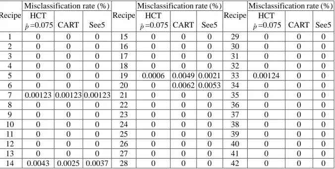
(8) List of Tables Table 2.1. The units and related subsystems of the 12 attributes ..............................30. Table 2.2. The 10-fold cross validation classification error rate of the 42-recipe. case ............................................................................................................31 Table 2.3 The misclassification rate  of the 42-recipe case.................................33 Table 2.4. The training time, classification time and 10-fold cross validation for the sum of classification error rates for different values of pˆ...............33. Table 2.5. The updating time of HCT when separation matrices change for different pˆ............................................................................................34. Table 2.6. The misclassified abnormal wafers caused by electrical spikes .............37. Table 3.1. The good enough vector of threshold values and the average overkill percentage of product A for three different rT ’ s .....................................60. Table 3.2. The good enough vector of threshold values and the average overkill percentage of product B for three different rT ’ s ....................................64. vi.

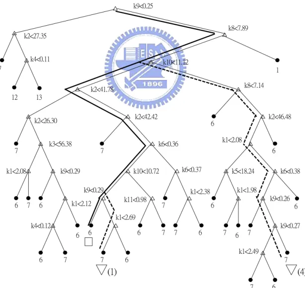
(9) List of Figures Figure 2.1. The structure of an ion implanter ............................................................6. Figure 2.2. The proposed fault detection and isolation scheme for the ion implanter................................................................................................8. Figure 2.3(a) Separable recipes ................................................................................11 Figure 2.3(b) Non-separable recipes ........................................................................11 Figure 2.4 Illustration of the separation between Ci and C j based on p j .......13 Figure 2.5(a). A separation matrix example [ D(Ci , C j ) k ] ..........................................14 1. Figure 2.5(b) A separation graph example resulted from the separation matrix in Figure 2.5(a) .....................................................................................14 Figure 2.6(a) The separation matrix [ D(Ci , C j ) k ] .....................................................14 2. Figure 2.6(b) Submatrix of. [ D (Ci , C j ) k 2 ]. corresponding to cluster A in Figure. 2.5(b) ................................................................................................14 Figure 2.6(c) Clusters split from cluster A using the submatrix shown in Figure 2.6(b) ................................................................................................14 Figure 2.7(a) The separation matrix [ D(C i , C j ) k ] ....................................................15 1. Figure 2.7(b) The separation matrix [ D(Ci , C j ) k ] ....................................................15 2. Figure 2.8. An example of using Algorithm I to build the clustering tree.............17. Figure 2.9. Using clustering tree to find the faulty attribute .................................28. Figure 2.10. The clustering tree of the 42-recipe case.............................................30. Figure 2.11. Classification tree of CART for TC4 ...................................................36. Figure 3.1. Flow chart of the real and simulated wafer testing procedures...........42. Figure 3.2. The structure of the OO theory based two-level algorithm.................51. Figure 3.3 Figure 3.4. Five types of standardized OPCs ........................................................52 The resulted ( E [V ] , E [R ] ) pairs of the 521 test wafers based on the vector of threshold values determined by two-level algorithm, random generator, three-sigma limit, six-sigma limit, GA and SA. Figure 3.5. algorithm..............................................................................................60 The resulted ( E [V ] , E [R ] ) pairs of the 590 test wafers based on the vector of threshold values determined by two-level algorithm, random generator, three-sigma limit, six-sigma limit, GA and SA algorithm..............................................................................................64. vii.

(10) Chapter 1 Introduction 1.1 Motivation Semiconductor manufacturing is a complex process that involves monitoring a great number of parameters from the early stages of the production to the packaging of an end product. The two most significant factors that determine the manufacturing performance are throughput and yield. The throughput and yield are the most important indexes for measuring the quality of semiconductor manufacturing process. Throughput is defined as the achieved unit output rate of a particular type of equipment asset. Yield is defined as the fraction of total input transformed into shippable output. The process of IC manufacturing often requires hundreds of sequential steps, each one of which could lead to yield loss. Consequently, maintaining product quality in an IC manufacturing facility often requires the strict control of hundreds or even thousands of process variables. Traditional statistical methods are no longer feasible nor efficient, if possible, in analyzing the vast amounts of data in a modern semiconductor manufacturing process. Traditional approaches have limits in extracting the full benefits of the data. Therefore, the manufacturing data is poorly exploited even in the most sophisticated processes. Small improvements on throughput and yield for tenths of a percent can save hundreds of millions of dollars annually in lost products, product rework, energy consumption, and the reduction of waste streams. Considering the big set of parameters and large volume of data in semiconductor manufacturing process, improving throughput and yield is indeed an extremely difficult. Thereofre, we narrow our focus of throughput and yield improvements on two issues: the fault detection and isolation of an ion implanter and reducing overkills and retests in wafer testing process.. 1.

(11) 1.2 Throughput and Yield Enhancement of Ion Implanter The semiconductor manufacturing process can be divided into four basic phases: wafer fabrication, wafer probe, assembly or packaging and final testing. Wafer fabrication is the most technologically-complex and capital-intensive phase among the four. In the wafer fabrication phase, ion implanter is a bottleneck machine in the semiconductor manufacturing process because of its expensiveness; thus, ion implantation is a critical operation to the throughput. The damaged wafer due to the malfunction of the ion implanter is not re-workable hence significantly affects the yield. Thus, the real-time fault detection and isolation for minimizing the possible down time of the ion implanter is a crucial issue in semiconductor manufacturing process.. 1.3 Throughput and Yield Improvement of Wafer Testing Semiconductor testing of ICs or chips is required at various stages during the fabrication process. Each IC must be individually tested in wafer and in packaged form to ensure that it functions as intended. Demand for testing products is driven by two considerations: new chip designs and higher unit volumes. As chips become increasingly powerful and complex, the need for high-speed and accurate testing becomes more important than ever. The process of testing individual chips in wafer form is referred to as wafer probing. Wafer probing establishes a temporary electrical contact between the chip and the automatic test equipment. This is the critical test for design and performance of the IC, and for sorting ICs before separation and costly packaging. A probing system, which transmits electrical signals to the wafer and analyzes the signals upon their return, has four principal components: the prober, the probe card, the probe station, and automatic test equipment. Although there exist techniques such as the Statistical Process Control (SPC) for monitoring the operations of the wafer probes, the probing errors may still occur in many aspects and cause some good dies being over killed, which will degrade the yield. Thus, reducing the number of overkills is always one of the main objectives in wafer testing process. The key 2.

(12) tool to identify or save overkills is retest, which is an additional wafer probing. However, retest is a major factor for decreasing the throughput. Thus, the overkill and the retest possess inherent conflicting factors, because reducing the former can gain more profit, however, at the expense of increasing the latter, which will degrade the throughput and increase the cost. Consequently, to save more overkills using less retests is a goal of the wafer testing process.. 1.4 Dissertation Outline This dissertation introduces two related issues on the throughput and yield of wafer fabrication and testing processes. The first issue is a fault detection and isolation problem of the ion implanter, and the second one is a reducing overkills under a tolerable retest level problem in wafer testing process. In Chapter 2, we propose a classification based fault detection and isolation scheme for the ion implanter. The proposed scheme consists of two parts: the classification part and the fault detection and isolation part. In the classification part, we propose a Hybrid Classification Tree (HCT) with learning capability to classify the recipe of a working wafer in the ion implanter, and a k-fold cross validation error is treated as the accuracy of the classification result. In the fault detection and isolation part, we propose a warning signal generation criteria based on the classification accuracy to detect and fault isolation scheme based on the HCT to isolate the actual fault of an ion implanter. We have compared the proposed classifier with the existing classification software and tested the validity of the proposed fault detection and isolation scheme for real cases and obtain successful results. In Chapter 3, we have formulated a stochastic optimization problem to find the optimal threshold values to reduce the overkills of dies under a tolerable retest level in wafer testing process. We have proposed an ordinal optimization (OO) theory based two-level algorithm to solve for a vector of good enough threshold values of the stochastic simulation optimization problem. In the first-level, we construct a crude but efficient model for the. 3.

(13) considered problem based on an artificial neural network. This crude model will then be used as a fitness function evaluation tool in a genetic algorithm to efficiently select N roughly good solutions from decision-variable space. In the second-level, starting from the selected N roughly good solutions we proceed with the existing ordinal optimization searching procedures to search a good enough solution of the considered problem. We have justified the quality of the obtained solution using simulations. We applied the proposed algorithm to the reduction of overkills and retests in a wafer testing process, which is formulated as a stochastic simulation optimization problem that consists of a huge decision-variable space formed by the vector of threshold values in the wafer testing process. The vector of good enough threshold values obtained by the proposed algorithm is very successful in the aspects of solution quality and computational efficiency. Finally, some conclusions for the dissertation are drawn in Chapter 4. We also suggest some possible future research issues concerning the methods developed in this dissertation.. 4.

(14) Chapter 2 Fault Detection and Isolation for the Ion Implanter 2.1 Introduction Ion implanter [1] is a bottleneck machine in the semiconductor manufacturing process because of its expensiveness; thus, ion implantation is a critical operation to the throughput. The damaged wafer due to the malfunction of the ion implanter is not re-workable hence significantly affects the yield. Therefore, a real-time fault detection to prevent more wafer damage and a fault isolation to reduce the down time of the ion implanter are crucial issues to the yield and throughput of the semiconductor manufacturing process. There are two categories of fault detection methods, the model based methods and model free methods. The model based methods, which utilize the mathematical model of the plant, originated from chemical process control, aerospace related research, and other areas have been developed in last three decades [2]-[4]. Model free methods, which do not use the mathematical model of the plant, range from physical redundancy, limit value checking [5] and spectrum analysis [6]. Among them, limit value checking method is widely used in practice. There are also two types of fault isolation methods [7], the classification methods and inference methods. If a-priori knowledge is not available for the relationships between the measured data patterns and faults, classification methods are used. For example, a neural network, trained using a large set of abnormal data pattern and known fault pairs, can be used to classify the corresponding fault of an abnormal data pattern. If there is a priori-knowledge for the relationships between faults and measured data patterns, a rule-based expert system can be used to inference the corresponding fault of an abnormal data pattern. Regarding fault detection, since there does not exist any proper models for the ion implanter, the model based fault detection methods cannot apply. Thus, the limit value checking method is currently employed in some semiconductor manufacturing companies.. 5.

(15) The structure of an ion implanter is shown in Figure 2.1 [1]. In general, the equipment supplier provides a digital equipment to monitor the proper operation of the scanning subsystem of the machine. The well-trained engineers employ the limit value checking method to investigate the SPC charts [8] of the measured parameters for other major subsystems, the ion source (filament), extraction electrode, mass analysis, and acceleration subsystems to monitor their operations. The measured parameters can be, for examples, filament voltage, filament current, discharge voltage,…, etc.. However, there are several tens to hundreds of recipes1 for wafer fabrication in a semiconductor foundry each day. Although the setting of scanning subsystem is independent of the recipes, the other four subsystems’parameters may vary widely due to various recipes. This induces the first drawback of the limit value checking method, that is the difficulty of defining a threshold to distinguish one recipe from the others. Since each recipe involves a combined setting of the four subsystems, this induces the second drawback of the limit value checking method that it cannot provide combination Analysis Magnet. Mass Anylysis Slit. Lens. Input Cassette Accelerator Scan System. Wafer. Extractor Output Cassette. Ion Source. Figure 2.1. 1. The structure of an ion implanter.. A recipe controls how vectors are initialized or changed during a process step. Examples include. recipe numbers which index tables of set points in furnaces, or written instructions to operators. A recipe is usually considered constant during any one process step. In this chapter, a recipe is corresponding to a specific product of integrated circuit.. 6.

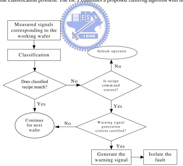
(16) information of the measured parameters of the four subsystems. In addition, the occurrence of electrical spikes in the ion implanter will make the measured parameters exceed the threshold and indicate a fault situation, however the electrical spikes are not actual machine faults. This is the third drawback of the limit value checking method. Regarding fault isolation, both classification methods and inference methods require a fairly large set of the abnormal data patterns with known faults to train a classifier and construct a rule-based expert system, respectively. Collecting a large set of abnormal data patterns with known faults in an ion implanter is very difficult, because there are several hundreds of steps in fabricating a chip and the chip failure is most probably known when it is under test. To find out which step in the complete manufacturing process causes the failure is already difficult not even mention the collection of a large set of abnormal data patterns with known faults due to ion implantation. Thus, the purpose of this chapter is to propose an automatic (i.e. no need of well-trained engineers) and effective tool to monitor the above mentioned four subsystems as a whole and generate a warning signal once a machine fault occurs and isolate that fault. To overcome the first two drawbacks of the limit value checking method, we should be able to identify the recipe of the working wafer from the measured parameters of all the four subsystems. This makes the data mining technique [9] attractive. To overcome the third drawback of the limit value checking method, we need to distinguish electrical spikes from the actual machine faults. Motivated by the above considerations, we propose a classification based fault detection and isolation scheme for the ion implanter. Viewing a recipe as a class, we can classify the recipe of the working wafer based on the corresponding measured parameters of the four subsystems. Thus, the overall structure of the proposed fault detection and isolation scheme can be shown in Figure 2.2. Our scheme starts from classifying the recipe of the working wafer based on the measured parameters. If the classified recipe of the working wafer matches its destined one, we assume there is no fault and proceed with next wafer. This no fault assumption may cause only few damaged wafers in the worst case. A detailed analysis of this claim will be addressed in Section 2.4. On the 7.

(17) other hand, if the classified recipe does not match its destined one, a double check of the recipe command should be carried out. If the command is wrong, the operator will be informed; otherwise, the warning signal generation criteria will be tested. If the criteria is satisfied, we conclude that there is a machine fault and a warning signal will be generated; otherwise, we will proceed with next wafer. Once a warning signal is generated, we will perform the fault isolation scheme to isolate the fault. In short, the proposed fault detection and isolation scheme consists of three major problems. The first one is a classification problem, which is to classify the recipe of a working wafer. The second one is a fault detection problem, which is to determine whether there is a machine fault and generate a warning signal if there is one. The third one is a fault isolation problem to determine which subsystem has a fault. In this chapter, we propose a Hybrid Classification Tree (HCT) with good learning capability to deal with the classification problem. The HCT combines a proposed clustering algorithm with the. M easured signals corresponding to the w orking w afer I n fo r m o p e r a t o r. C lassification No No. Does classified recipe match?. Is r e c ip e c om m a n d c or r e c t?. Y es. Continue for next wafer. Y es. W arn in g s ign a l g e n e r a t io n c r it e r i a s a t is fi e d ?. No. Y es G enerate the w arning signal. Figure 2.2.. Isolate the fault. The proposed fault detection and isolation scheme for the ion implanter. 8.

(18) Classification and Regression Tree (CART) [10] to take the advantages of the specific setting of a recipe during a process step. Its good learning capability will enable it to work on line. Since the operator should interrupt wafer processing immediately when a fault is detected, a high standard in the accuracy of fault detection is required so as not to unnecessarily degrade the throughput. Thus, to account for the possible inaccuracy caused by the HCT, we propose a warning signal generation criteria to deal with the fault detection problem. This criteria aims to minimize the probability of false alarm when there is no fault as well as the probability of no alarm while fault exists; the former tries to eliminate the indicated fault situations due to electrical spikes and classification errors, while the latter tries to find out the hidden machine faults when classified recipe matches the destined one; however, we need not worry about the latter one by the no fault assumption mentioned above. To cope with the fault isolation problem, we propose an HCT based fault isolation scheme. The basic idea of this scheme is to find the parameter (or parameters) that causes the classification errors. Dislike the existing methods, which need to collect a fairly large set of measured data patterns with known faults as indicated earlier, the proposed fault isolation scheme almost spend no extra effort as will be seen in Section 2.3.2. From here on, we will use the terminologies attribute and data pattern in classification techniques to represent the parameter and data of the measured parameters of the four subsystems of the ion implanter, respectively. We organize chapter 2 in the following manner. In Section 2.2, we will present the HCT and its learning capability. In Section 2.3, we will analyze the probability of no alarm while machine fault exists to verify the no fault assumption and present the criteria for generating the warning signal. We will also present the fault isolation scheme in this section. In Section 2.4, we will apply the HCT to real data sets to obtain the k-fold cross validation classification errors, based on which, we will demonstrate the validity of the proposed warning signal generation criteria and the fault isolation scheme. In the meantime, we will also investigate the learning capability of HCT by reporting the computation time needed to update the classification rules of HCT. In Section 2.5, we will make a conclusion. 9.

(19) 2.2 The Hybrid Classification Tree (HCT) There exist numerous classification techniques for classification problems of continuous attributes such as the neural network approach [11], maximum-likelihood approach [12], fuzzy set theory based approach [13], decision tree [14], CART [10], kernel based learning algorithms [15], and recent methods like random forests [16], multiple additive regression trees (MART) [17] and the boosting flexible learning ensembles with dynamic feature selection technique [18], etc.. Among them, the neural network approach is superior in the aspects of free data distribution and free data importance, however they are computationally expensive and produce variable results due to the random initial weights. The maximum-likelihood approach was the most widely used method in classifying remotely measurement data, however its performance was degraded when the target classes could not be adequately described by the statistical model. The fuzzy set theory based approach had been successfully applied to the pattern classification problem, however the computational complexity is raised when the number of classes as well as the number of attributes are large. Decision tree is mainly designed for classification of discrete variables. However, CART can handle continuous attributes. Compared with random forest, MART and boosting flexible learning ensembles with dynamic feature selection technique, disadvantage of CART is inaccuracy due to its nature of piecewise constant approximation. However, the biggest advantage of CART is its interpretability whereas the above mentioned three methods and the kernel based learning algorithms are thought to lack this feature. The interpretability is the key feature of our HCT based fault isolation scheme, however, at the expense of some classification accuracy. Fortunately, the decrease in accuracy will be remedied by the warning signal generation criteria as for applying to the fault detection of the ion implanter, which will be presented in Section 2.3.1. The tree sizes of CART are closely related to the interpretability and accuracy. Small tree can be easily interpreted, while the interpretability of a large tree is questionable. On the other hand, larger tree is more accurate than the smaller one. Thus, to retain the interpretability of a small tree while keeping the accuracy of a large tree, we intend to propose a preprocessing step to reduce the tree size of CART so as to improve the interpretability while keeping its classification accuracy. In. 10.

(20) general, a recipe may contain various steps, and a recipe step remains constant during the processing of one wafer, however different attributes (parameters) may be ramped during the entire processing step. Nonetheless some (not all, as can be observed from the experimental results shown in Figure 2.10) attributes’mean of each individual recipe step are still a key to distinguish the recipes. Thus, we can exploit this property to fulfill the above mentioned objective of preprocessing. To do this, we propose a separation matrix based clustering algorithm as a preprocessing step for CART. This clustering algorithm will classify the whole data set into a clustering tree and the classes in the leaf clusters will be classified by the CART. Because both the size and the number of classes of the leaf cluster are much smaller than the original data set, the computational complexity of CART can be improved.. 2.2.1 The Separation Matrices Based Clustering Algorithm Due to the above mentioned property of a recipe during a processing step, we can investigate the separability between two recipes through the degree of overlapping of the attribute-values. For example, suppose the probability density function of an attribute for the two recipes A and B are as shown in Figure 2.3(a), then these two recipes are separable based on that attribute; while in the case of Figure 2.3(b), the two recipes are not. Throughout this section, we will use the terminology class in classification techniques to represent recipe. p(x) (probability density). B. A. (value of an attribute). x. Figure 2.3(a).. Separable recipes.. p(x) (probability density). A. B (value of an attribute). x. Figure 2.3(b).. Non-separable recipes. 11.

(21) 2.2.1.1. Chebyshev Inequality Based Separation Matrices. We let D(Ci , C j ) k denote the separation index between classes Ci and C j based on attribute k and define 0, if Ci and C j are separable based on attribute k,  D(Ci , C j ) k  1, otherwise.. (2.1). Clearly, D(C i , C i ) k 1 and D(C i , C j ) k D(C j , Ci ) k for any attribute k . The value of D(Ci , C j ) k is computed using Chebyshev inequality [19] as described below. We let the. random variable X ik denote the k th attribute of class C i , and let ik and ik denote the mean and standard deviation of X ik , respectively. Let a ik be a positive real number. )] denotes the probability of the event ( ) , and such that P[ X ik ik a ik ] , where P[(  is a small real number representing low probability, which is usually set to be 0.05. The value of a ik corresponding to a given  can be calculated from setting  ik aik  using 2. Chebyshev inequality. Without loss of generality, we can assume ik kj . We let. . . k p j min(1, kj max(, kj ik aik ) ) , where a i is defined above and  is a very small 2. positive real number to avoid the denominator of the square term being 0 or negative. p j is an upper bound of P[| X kj kj |max(, kj ik aik )] based on Chebyshev inequality. If. kj is sufficiently larger than ik a ik , p j will be very small, which implies the overlapping of the classes C i and C j on attribute k will be very small; consequently the classes C j and C i are more likely to be separable as illustrated in Figure 2.4. Therefore, we can define a threshold value pˆ, such that the separation index for classes C i and C j can be calculated by the following: 0, if p j pˆ,  D(Ci , C j ) k  1, otherwise.. (2.2). Now we can define [ D(Ci , C j ) k ] as the separation matrix for all classes based on attribute k , whose ( i, j ) th entry is D(Ci , C j ) k .. 12.

(22) p( xk ) (probability density) (value of the k th attribute).  k i. Figure 2.4.. 2.2.1.2. aik.  k j. xk. Illustration of the separation between C i and C j based on p j .. Splitting Cluster Using Separation Matrices. We let Cr0 denote the root cluster, which represents the whole data set. Treating each class in Cr0 as a node, we can view [ D(Ci , C j ) k1 ] as an incidence matrix for all nodes in Cr0 based on attribute k1 . That means nodes C i and C j will be connected by an arc if D(Ci , C j ) k1 1 . The graph constructed based on a separation matrix is called a separation graph,. which may contain separate connecting sub-graphs. Each connecting sub-graph represents a cluster of non-separable classes based on attribute k1 , and the number of disjoint sub-graphs represent the number of disjoint clusters that can be split from Cr0 using attribute k1 . For example, the separation graph constructed from the separation matrix [ D(Ci , C j ) k1 ] given in Figure 2.5(a) is shown in Figure 2.5(b), which consists of two disjoint clusters, or two separate connecting sub-graphs, A and B. The resulted clusters can be further split by other attributes. For example, cluster A in Figure 2.5(b) can be further split by attribute k 2 , whose [ D(Ci , C j ) k 2 ] is shown in Figure 2.6(a), in the following manner. Collecting the rows and. columns of [ D(Ci , C j ) k 2 ] corresponding to the classes in cluster A to form the submatrix shown in Figure 2.6(b). Repeating the same process of splitting Cr0 using [ D(Ci , C j ) k1 ] , cluster A can be split into two clusters C and D as shown in Figure 2.6(c) by using the submatrix shown in Figure 2.6(b).. 13.

(23) C1 C2 C3 C4 C5 C6. Figure 2.5(a).. A separation matrix example [ D(Ci , C j ) k1 ] .. A : B :. Figure 2.5(b).. C1 C2 C3 C4 C5 C6 1 1 0 0 0 0 1 1 1 0 0 0 0 1 1 0 0 0 0 0 0 1 1 0 0 0 0 1 1 1 0 0 0 0 1 1. C1. C2. C3. C4. C5. C6. A separation graph example resulted from the separation matrix in Figure 2.5(a).. C1 C2 C3 C4 C5 C6. Figure 2.6(a).. C1 C2 C3 C4 C5 C6 1 0 0 0 0 0 0 1 1 0 0 0 0 1 1 1 0 0 0 0 1 1 1 0 0 0 0 1 1 1 0 0 0 0 1 1. The separation matrix [ D(Ci , C j ) k 2 ] . C1 C2 C3 C1 1 0 0 C2 0 1 1 C3 0 1 1. Figure 2.6(b).. Submatrix of [ D(Ci , C j ) k 2 ] corresponding to cluster A in Figure 2.5(b). C : D :. Figure 2.6(c).. 2.2.1.3. C1 C2. C3. Clusters split from cluster A using the submatrix shown in Figure 2.6(b).. The Choice of Attributes for Cluster Splitting and the Construction of the Clustering Tree. Because the separation matrix has already indicated certain distribution of the attribute values of all classes, we can employ a coarser partition like fuzzy intervals to classify the disjoint clusters instead of treating each continuous value as a discrete one like CART. In. 14.

(24) general, for a given range of attribute values, more finer fuzzy partition is needed to classify a cluster with larger number of classes. In other words, for a given fuzzy partition and the range of attribute values, the classification will be more accurate for a cluster with smaller number of classes. Considering that any inaccurate cluster splitting will influence the accuracy of the subsequent cluster splitting along the tree path, we set the criteria for choosing the attribute to split a cluster as minimizing the multiplication of the average number of classes and the variation of the number of classes in the resulted child clusters. This criteria implies that the attribute which results in more child clusters and smaller variation in the number of classes in the child clusters is preferred. For example, for the separation matrices of two attributes shown in Figure 2.7(a) and 2.7(b), suppose that we use the attribute k1 to split the cluster first, we obtain three child clusters. One consists of 1 class, and the other two consist of three and four classes. While if we use attribute k 2 first, we will obtain four child clusters, and each child cluster contains two classes. Based on the criteria indicated above, we would choose. k 2 to split the cluster. To put this criteria into a mathematical form, we let Lk and nk , l (Crj ) denote the number of child clusters and the number of classes in the l th child cluster resulted. C1 C2 C3 C4 C5 C6 C7 C8. Figure 2.7(a).. The separation matrix [ D(C i , C j ) k ] . 1. C1 C2 C3 C4 C5 C6 C7 C8. Figure 2.7(b).. C1 C2 C3 C4 C5 C6 C7 C8 1 0 0 0 0 0 0 0 0 1 1 0 0 0 0 0 0 1 1 1 0 0 0 0 0 0 1 1 0 0 0 0 0 0 0 0 1 1 0 0 0 0 0 0 1 1 1 0 0 0 0 0 0 1 1 0 0 0 0 0 0 0 1 1. C1 C2 C3 C4 C5 C6 C7 C8 1 1 0 0 0 0 0 0 1 1 0 0 0 0 0 0 0 0 1 1 0 0 0 0 0 0 1 1 0 0 0 0 0 0 0 0 1 1 0 0 0 0 0 0 1 1 0 0 0 0 0 0 0 0 1 1 0 0 0 0 0 0 1 1. The separation matrix [ D(Ci , C j ) k ] . 2. 15.

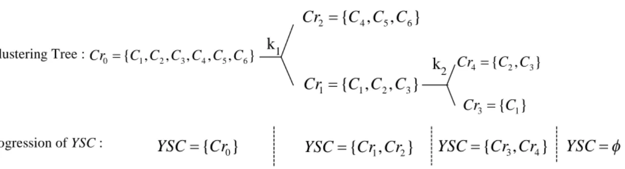
(25) from using attribute k to split the cluster Cr j , respectively. Then, the criteria for choosing the attribute for splitting Cr j is  Lk  min  nk , l Crj  k l 1 . .   L. Lk    nk , l (Crj ) nk , l Crj k   l 1.  L. 2. k.       . (2.3). where the first term inside the big bracket represents the average number of classes in the resulted child clusters and the second term denotes the variance of the number of classes in the resulted child clusters, where n k , l  Crj  n k , l  Crj Lk . Lk. l 1. Now, our algorithm for choosing the splitting attribute to build the clustering tree can be stated as follows.. Algorithm I: Choose the splitting attributes and build the clustering tree. Step 0: Given the original data set Cr0 and the separation matrices of all attributes. Set Cr0 as the root cluster and define the set of Yet Split Clusters (YSC)={ Cr0 }. Step 1: For each cluster in YSC, obtain the corresponding splitting attribute k based on the criteria (2.3). Using the obtained attribute to split the cluster, and put the resulting child clusters into YSC. Discard the clusters that had been split and the clusters that cannot be split using any attribute. Step 2: If YSC , stop; otherwise return to Step 1.. Figure 2.8 shows a clustering tree built by using the separation matrices of two attributes shown in Figure 2.5(a) and 2.6(a) to split the root cluster Cr0 ={C1,C2,C3,C4,C5,C6}. Algorithm I uses three iterations to build the tree. The splitting attribute for each cluster and the progression of YSC are also shown in this figure. We define the leaf cluster in the clustering tree as the Terminal Cluster (TC) . Each TC may contain one class only or several classes, which cannot be split further using any attribute. For the purpose of classifying a new data pattern into a TC, we need to use the splitting. 16.

(26) attributes to construct the cluster splitting rules for each cluster in the clustering tree based on the fuzzy rules [20] for single attribute as presented in the following section. It should be noted that the fuzzy rules employed here are for single attribute, thus we can circumvent the computational complexity of the fuzzy set theory based approach indicated in Section 2.2. Cr2 {C 4 , C5 , C6 } Clustering Tree : Cr0 {C1 , C2 , C3 , C4 , C5 , C6 }. k1 Cr1 {C1 , C2 , C3 }. Progression of YSC :. Figure 2.8.. YSC {Cr0 }. YSC {Cr1 , Cr2 }. k2 Cr4 {C2 , C3 } Cr3 {C1}. YSC {Cr3 , Cr4 }. YSC . An example of using Algorithm I to build the clustering tree.. 2.2.1.4 The Clustering Algorithm The separation matrix based clustering algorithm consists of two parts: the training part and the classification part. The training part, which is prepared for the classification part, consists of three steps: (i) construction of the separation matrices for all attributes, (ii) determine the cluster splitting attribute and build the clustering tree, and (iii) throughout the clustering tree, generate the fuzzy if-then rules needed to classify a data pattern into proper child cluster based on a given set of training data patterns with known TCs. In the above three steps, (i) and (ii) had been presented in previous subsections. The details of (iii) as well as the classification part are described below.. 1. The Fuzzy-Rule Generation Procedures of the Clustering Algorithm The fuzzy rules for splitting a non-TC cluster using the corresponding splitting attribute in our clustering algorithm are of the same type. Thus, for the sake of explanation, we will focus on generating the fuzzy rules for one cluster in the clustering tree. We let Cr j denote a non-TC cluster and k denote the corresponding splitting attribute. We let xks , s 1,..., g , denote the k th attribute of g data patterns, x s , s 1,..., g , from M j known child clusters,. 17.

(27) CCr j1 ,..., CCr jM j . These g data patterns form the training data set for splitting Cr j . The fuzzy. rules for splitting cluster Cr j are of the following type. For i 1,..., K , where K denotes the number of fuzzy partitioned intervals on the range of the k th attribute values, Rule Ri (Crj ) : If xks is AiK , then the x s belongs to CCrji with CFi K , where AiK is the i th partitioned fuzzy interval, CCrji is the consequent, i.e. one of the M j child clusters, and CFi K is the grade of certainty of rule Ri (Crj ). (2.4). What need be determined in the above rule are CCrji and CFi K , and the procedures for determining them are called fuzzy rules generation procedures for splitting one cluster as described below. K. Let AiK be characterized by the nonnegative fuzzy membership function f i ( ) . The K. membership function f i ( ) can be triangular, Gaussian, or any other shape. In this chapter, K. we consider the triangular membership function. Then, f i ( xks ) can be considered as the grade of compatibility of xks with respect to AiK . We define. CCrjl ( Ri (Crj )) . f. K i. ( xks ). (2.5). x s CCrjl. as the sum of grade of compatibility of child cluster CCrjl with respect to AiK . Then the algorithm for generating fuzzy rules for splitting cluster Cr j can be stated as follows:. Algorithm II: Generation of the K fuzzy rules for splitting cluster Cr j . Step 0: Given g training data patterns x s , s 1,..., g , with known child clusters CCrjl , l 1,..., M j of the to-be-split cluster Cr j and the corresponding splitting attribute k .. Set i 1 . Step 1: Calculate the sum of grade of compatibility of child cluster CCrjl , l 1,..., M j , with respect to AiK by (2.5).. 18.

(28) Step 2: Find the child cluster CCrjx such that. CCr jx ( Ri (Crj )) max{CCr j 1 ( Ri (Crj )),  , CCr jM ( Ri (Crj ))}. (2.6). j. then CCrjx is the consequent CCrji in rule Ri (Crj ) . Step 3: Determine CFi K , the grade of certainty of rule Ri (Crj ) , by. . CFi K  CCrjx ( Ri (Crj )) ( Ri (Crj )). where ( Ri ( Cr j )) . . CCr jl CCr jl CCr jx.  M. l 1. CCrjl. ( Ri (Crj )). (2.7). ( Ri ( Cr j )) ( M j 1) denotes the average of the sum. of grade of compatibility of the rest of child clusters with respect to AiK . Step 4: If i K , stop; else, set i i 1 , and return to Step 1.. 2. Training Part of the Clustering Algorithm Combining the construction of separation matrices, determination of the splitting attributes, building of the clustering tree and the above fuzzy rule generation procedures, we are ready to summarize the training procedures of the clustering algorithm using the training data set.. Algorithm III: Training procedures of the clustering algorithm. Step 0: Given a set of training data patterns with known classes; compute ik and ik of each class. Ci. and each attribute. k ; compute the separation matrices. [ D(C i , C j ) k ] based on (2.2) for each attribute k .. Step 1: Apply Algorithm I to obtain the splitting attributes and build the clustering tree. Step 2: Use Algorithm II to generate the fuzzy rules for each cluster in the clustering tree.. 3. Classification Part of the Clustering Algorithm Once the fuzzy rules for splitting the clusters in the clustering tree are generated, we can determine the child cluster to which the new data pattern belongs at each cluster based on a 19.

(29) fuzzy reasoning method. corresponding to the Let the new data pattern be xand let x k be the k th attribute of x. splitting attribute k at cluster Cr j . We define CCr jl , the weighting grade of certainty of x k with respect to the child cluster CCrjl , as the sum of the multiplication of the grade of K compatibility of x and the grade of certainty of rule Ri (Crj ) over all k with respect to Ai. K trained rules whose consequent are CCrjl . We can express CCr jl mathematically as. f. CCr jl . ( x ) CFi K . Then the classification procedures for the new data can be. K i k Ri ( Cr j ), CCr ji CCr jl. stated below. Classification Procedures: The child cluster CCrjy , with respect to which the weighting grade of certainty of. x is k. maximum, is the concluded cluster of. x, that is,. CCrjy arg(max{CCr j 1 ,, CCr jM }) . j. Now, the classification procedures for classifying a new data pattern xinto a TC can be stated in the following.. Algorithm IV: Classification procedures of the clustering algorithm. Step 0: Given a new data pattern x ( x1 ,..., x n ) , where n denotes the total number of attributes; set Present Cluster (PCr)= Cr0 . Step 1: Use x k , where k corresponds to the attribute used for splitting the PCr, and the classification procedures stated above to classify xinto a child cluster of PCr, we denote this child cluster by CPCr. If the CPCr is not a TC, set PCr=CPCr and repeat this step; otherwise, stop.. 2.2.2 The CART for Terminal Cluster (TC) The TCs resulted from the training part of the separation matrix based clustering algorithm may consist of one or more classes. Since the number of classes and the size of the corresponding data set in each TC should be much smaller than Cr0 , it will be 20.

(30) computationally much easier to apply CART to classify the TCs and the resulting tree size of each TC will be much smaller. Therefore, our clustering algorithm help reduce the computational complexity and the tree size of CART when applies to Cr0 alone. The CART is a well-developed classification tool. The details of this classification technique can be found everywhere [10]. Similar to the proposed clustering algorithm, CART also consists of training and classification parts. The training part of CART is to build a classification tree and the splitting rules in each node. In brief, the construction of a CART classification tree and splitting rules centers on three major elements: (a) the splitting rule, (b) the goodness-of-split criteria, and (c) the criteria for choosing an optimal or final tree for analysis. Regarding (a), there are three major splitting rules in CART. The one we employed here is the Gini’ s criteria [10]. This criteria starts the tree-building process by partitioning the TC into binary nodes based upon a very simple question of the form: is k b ? where k is an attribute and b is a real number. Regarding (b), the CART uses a. computation-intensive algorithm that searches for the best split at all possible split points for each attribute that decrease the Gini’ s impurity measure most. CART will recursively apply this splitting rule to split non-terminal child nodes at each successive stage. In order to reduce the complexity of the built tree which is measured by the number of its terminal nodes, CART uses a pruning process to find an optimal tree as pointed out in (c). The computational complexity of the training part of CART mainly lies in the exhaustive search for the best split required in (b). Once the classification tree and the splitting rules are obtained, the classification procedure of CART is simply asking whether k b ? to determine which of the binary child nodes the new data pattern belongs to throughout the classification tree.. 2.2.3 Classification of a New Data Pattern Once the training part of the HCT, which combines the training parts of the clustering algorithm and CART, is completed, we are ready to use the classification procedures of both. 21.

(31) clustering algorithm and CART to classify a new data pattern as required in the first two blocks in Figure 2.2.. 2.2.4 Learning Capability The learning capability of a classifier is very important in current application, because for every fourteen minutes, 24 wafers (or a lot) of the same recipe will be ion implanted. Thus, new data patterns arrive with a high frequency. For the sake of explanation, we can assume the recipe of the working wafer is one of the recipes under work, because only slight modification is needed for the case of new recipe. The learning of HCT after the new data pattern joins in consists of two parts. The first part is for the clustering algorithm and the second part is for CART. Learning of the clustering algorithm consists of three updating steps: (i) updating the separation matrices, (ii) updating the attributes used to split clusters as well as the clustering tree, and (iii) updating the fuzzy rules for splitting clusters. Learning of CART is just to update the best split for each node in the classification tree.. 2.2.4.1 Learning of the Clustering Algorithm Since the new lot of wafers is of the same recipe, the new data patterns will be used to update the mean and variance of each attribute of the corresponding class. Denoting the class index of the new data pattern by m , then we will update mk and mk for all k , which will be used to update the separation indices D(Cm , C j ) k for all j , all k . Suppose the updated D(Cm , C j ) k do not change for all j and all k , then the separation matrices remain the same; consequently, the splitting attributes for clusters and the clustering tree also remain the same as can be observed from Algorithm I. This implies that if the separation matrices are unchanged after the new data pattern joins in, the updating step (ii) can be skipped. In fact, mk and mk will only slightly deteriorate when the new data pattern join in because of the large amount of training data set. This implies that the updated separation matrices may change only when the amount of accumulated new data patterns. 22.

(32) are large enough. On the other hand, suppose D(Cm , C j ) k changes for any j and k , and cause the corresponding separation matrices changed in updating step (i), we need to proceed with updating step (ii) by performing Algorithm I (i.e. Step 1 of Algorithm III) to update the splitting attributes and the clustering tree. To update the fuzzy rules indicated in the updating step (iii), we also consider two cases. In the case of unchanged separation matrices, which implies the clustering tree and splitting attributes remain the same, we only need to update the fuzzy rules for the clusters in the tree path of the clustering tree, along which the new data pattern belongs to. To do so, we let Crj be a non-TC cluster in this tree path, and let CCrjz be the child cluster of Crj in this. tree path. To update the rules Ri (Crj ) in (2.4) is to update the consequent and grade of certainty after the new data pattern join in. To update the consequent, we need to update. CCrjz ( Ri (Crj )) first. To do so, we need to add an extra term of the nonnegative membership function of the new data pattern on the right hand side of (2.5). The updated. CCrjz ( Ri (Crj )) will be larger than the original one. Thus according to Step 2 of Algorithm II, the consequent will not be changed. Subsequently, we can use the updated. CCrjz ( Ri (Crj )) to update the corresponding CFi K by (2.7). Thus, in this case, updating fuzzy rules is an easy task because the length of a tree path in the clustering tree is usually short. In the case if the clustering tree or any splitting attributes changes due to the changed separation matrices, we need to perform Step 2 of Algorithm III, which is Algorithm II, to update the fuzzy rules. Of course, this is more complicated than previous case. However, no matter what case, it will not affect HCT to work real-time and on-line as will be demonstrated in Section 2.4.. 2.2.4.2 Learning of CART Following from previous discussions, there are also two cases for updating the splitting rules of CART. The first case is a subsequent situation of the unchanged separation matrices such that the TCs of the clustering tree do not change. Since the number of training data. 23.

(33) patterns are very large, the best split point of each attribute in each node of the CART will alter at most slightly when new data pattern join in. Therefore, we need not exhaustively search for the split point of each attribute. Instead, we can search for the split point only within a window of the original best split point of each attribute. The window is set to be w discrete points at the best split point of each attribute. This will of course save a lot of computation time. In addition, we need only update the splitting rules for just one TC, to which the new data pattern belongs. The other case is when the separation matrices change and cause the clustering tree changes. In this case, we will rerun the CART for all TCs. As indicated at the end of previous subsection, this will not affect HCT to work real-time and on-line.. 2.3 Warning Signal Generation and Fault Isolation. 2.3.1 Warning Signal Generation In general, the ion implanter will be stopped whenever there is a warning signal so as not to damage the subsequent wafers. However, this reaction will be justified only when the warning signal is absolutely correct; otherwise, the throughput will be degraded. Thus, to minimize the probability of false alarms should be one of the objectives. On the other hand, thousands of wafers may be damaged if any fault is not detected. Thus, to minimize the probability of overlooking a fault is another objective. In general, a matched classification result implies (i) the machine is in normal condition, or (ii) the actual implantation has been wrong due to a machine fault but a misclassification makes the classified recipe match the destined one. Case (ii) indicates a fault situation that cannot be observed from the matched result. We let i denote the misclassification rate of recipe i , which can be calculated by the following. i ( j )m(i | j ) j i. 24. (2.8).

(34) where ( j ) denotes the prior probability of recipe. j and m(i | j ) denotes the. misclassification rate of classifying recipe j to be recipe i . If case (ii) occurs to recipe i , then the probability of a series of n such events occur is i . This indicates the n. probability of an undetected machine fault will be extremely small provided that i is small, and n is large. This also implies that the matched recipe will eventually mismatch provided that the matched result is due to a misclassification. Real values of i for all i based on HCT will be given through the tests presented in Section 2.4. This addresses the comment cited in Section 2.1 that we need not check the existence of a machine fault when the classified recipe matches the destined one, and the cost of such a reaction is at most n damaged wafers, where n is a positive integer that makes in extremely small. This also indicates when the classified recipe matches the destined one, we can continue for next wafer as shown in Figure 2.2. Thus, using the classification accuracy of the HCT as the basis of generating a warning signal, our objective can be simplified to minimizing the probability of false alarm. There are two causes of false alarms. One is the electrical spike and the other is the classification error. Both cases will cause the classified recipe mismatch the destined one and require the checking of warning signal generation criteria as indicated in Figure 2.2. To minimize the probability of false alarm due to an electrical spike, we should distinguish an electrical spike from a machine fault. The electrical spike is only temporary, which may affect one or two wafers only, while the machine fault will last until it is fixed. Thus, an easier way to distinguish them is checking whether a series of classification errors occur. In other words, if there are more than, say, four consecutive classification errors, the causes of the errors should not be the electrical spikes. Similar reasons apply to the classification errors. We let qi denote the classification error rate, which is defined as (number of misclassified wafers/number of test wafers)*100%, of recipe i obtained using k-fold cross validation. Then the probability of the occurrence of n consecutive classification errors is ( qi ) n , which decreases sharply when n increases. Thus, an easier way to distinguish the. classification error from the machine fault is also checking whether a series of classification 25.

(35) errors occur. To achieve this, we can predetermine a very small positive real number , a probability indication of an event that is almost not possible to occur. Then if ( qi ) n , we can conclude that the cause of mismatched recipe is not classification errors. Thus we can state our warning signal generation criteria as follows. Let the classification error rate of recipe i obtained using k-fold cross validation be denoted by qi , and let n denote the number of consecutive working wafers, then the proposed criteria for generating a warning signal is: Assume the classified recipe of the (l 1) th wafer matches the destined one, while the l th, (l 1) t h, …,(l n ) th wafers do not, the warning signal will be generated at the (l n ) th wafer provided that the following two conditions hold:. qil (l ) qil 1 (l 1)    qil n (l n) . (2.9). n n1 ,. (2.10). and. where il denotes the destined recipe of the l th wafer, qi (l ) denotes the qi of the l th wafer,  is a very small positive real number, and n1 denotes the maximum number of consecutive wafers that can be affected by the electrical spikes.. If condition (2.9) holds, we can exclude the possibility of false alarm due to classification errors. If condition (2.10) holds, we can exclude the possibility of false alarm due to the electrical spikes.. 2.3.2 Fault Isolation To eliminate the machine fault, we need to isolate the fault first. In general, when there is. 26.

(36) a fault in a subsystem, the attribute (or attributes) corresponding to that subsystem may become abnormal. Thus, the basic idea of our fault isolation scheme is to find the attribute(s) that causes the classification errors, and this can be easily done in a single-tree classifier like CART and HCT, which is their biggest advantage, the interpretability. In fact, the tree-structure of HCT is much simpler than CART, because it largely reduces the tree size of CART by using the clustering tree to separate the whole data set into several TCs. Thus, if the misclassified recipe and the destined recipe belong to different TCs, we can use the clustering tree to find the faulty attribute. While if they belong to the same TC, we will use the corresponding CART to find the faulty attribute. Considering that the machine fault may occur abruptly or develop gradually, and there may be single or multiple faulty attributes, we will find the faulty attribute(s) for each misclassified wafer by the aid of its tree path and the tree paths of several latest correctly classified wafers of the same destined recipe. Thus, once a warning signal is generated, our fault isolation scheme will proceed as follows.. Step 1: Collect the m1 consecutive misclassified wafers that cause the warning signal, i.e.. m1 max(n, n1 ) such that conditions (2.9) and (2.10) hold. Step 2: Collect the latest m2 correctly classified wafers, which have the same destined recipes as the m1 wafers in Step 1. Step 3: For each of the m1 wafers in Step 1 and each of the m2 wafers in Step 2, we will find the faulty attribute(s) that causes the misclassification as follows. 3.1 Suppose the two wafers belong to different TCs, say TCi and TCk , we will use the clustering tree to find the faulty attribute by tracing the tree paths backward from the corresponding TCs. These two paths will meet at a node whose splitting attribute will be the faulty attribute. As illustrated in Figure 2.9, the faulty attribute is k1 . 3.2 Suppose the two wafers belong to the same TC, and they lie in two different terminal nodes of the corresponding CART, we can find the faulty attribute in a similar manner as in Step 3.1 using the classification tree of CART. 27.

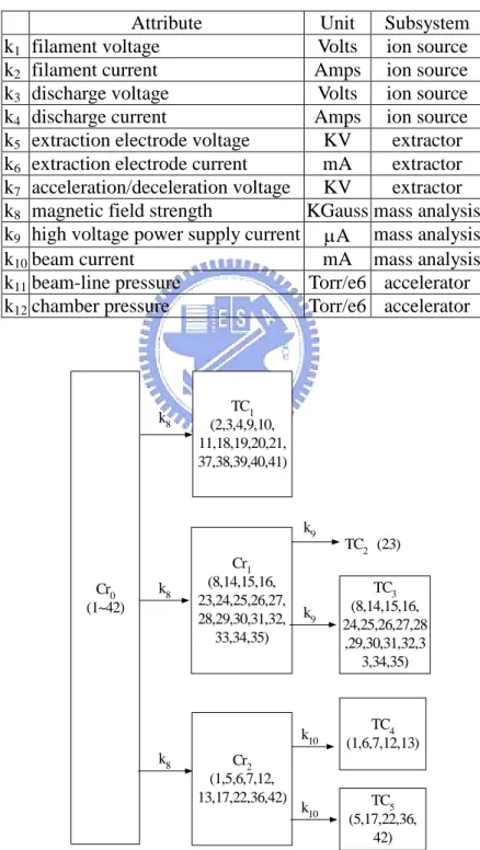
(37) Step 4: List all the different faulty attributes found from the m1 m2 searches in Step3 and calculate the corresponding probability, based on the frequency of occurrences. Indicate the corresponding subsystem of the faulty attributes and calculate the corresponding probability by adding the probabilities of the faulty attributes in this subsystem.. k1. k2. TCi Figure 2.9.. k3. .... .... TCk. .... Using clustering tree to find the faulty attribute.. 2.4 Test Results of HCT, Warning Signal Generation and Fault Isolation. 2.4.1 Test Results of HCT In general, there are quite a few attributes that can be measured from the ion implanter; however, not all attributes are helpful in classification. According to the domain knowledge, the following 12 attributes, k1, …,k11 and k12, are recommended: filament voltage, filament current, discharge voltage, discharge current, extraction electrode voltage, extraction electrode current, acceleration/deceleration voltage, magnetic field strength, high voltage power supply current, beam current, beam-line pressure, and chamber pressure, respectively. These 12 attributes cover the four subsystems of the ion implanter. Table 2.1 shows the units and related subsystems of the above 12 attributes. We have made all the tests on a 26-recipe case and a 42-recipe case. Due to the page limitation, we will present the complicated 28.

(38) 42-recipe case only. It should be noted that all the test results shown in this section are simulated in a Pentium IV PC using Matlab. A data set of 42-recipe case, and each recipe consists of a thousand to 10,000 wafers are supported from a local world-renowned foundry. We use them to test the classification accuracy of the proposed classifier HCT and to demonstrate the validity of the warning signal generation criteria and fault isolation scheme. It takes one second to measure a 12-attribute data pattern. The ion implantation time for a wafer is around 10 seconds. Thus, ten data patterns are taken while a wafer is under work. The wafer changeover time is 26 seconds on average. Each lot contains 24 wafers, and the setup time for a new lot is 13 minutes. For all the measured data patterns in this case, we randomly divide them in wafer base into ten parts. We take 9 parts as training data set and 1 part as test data set. We set pˆ0.075 in (2.2), the number of fuzzy partitioned intervals K 12 and a triangle K. nonnegative membership function for f i ( ) in Algorithm II. Applying Algorithm III to the training data set, the resulting clustering tree and the splitting attributes are shown in Figure 2.10, where each cluster is denoted by a block, and the recipes contained in a cluster are shown inside the parenthesis in each block. The attribute used for splitting each cluster is indicated at the outgoing branch in the clustering tree. The corresponding fuzzy rules for each splitting attribute are also obtained. There are five TCs, and each TC consists of more than one recipe except for the one consisting of recipe 23 only. Subsequently, we apply CART to the four TCs and build the classification tree and splitting rules for each TC. We then use the part of test data to test the trained HCT using Algorithm IV of the clustering algorithm and the classification tree and splitting rules of CART. Since each wafer corresponds to 10 measured data patterns, and each test data pattern will be classified to a recipe, thus a majority voting scheme is used to conclude the classified recipe of the wafer corresponding to the 10 test data patterns. Repeating this process for ten times by circulating the training data set and test data set, Table 2.2 shows the resulting 10-fold cross validation classification error rate of all recipes in this test. We also indicate the 10-fold cross validation classification error rate using the software See5 [21] and CART [10] in this 29.

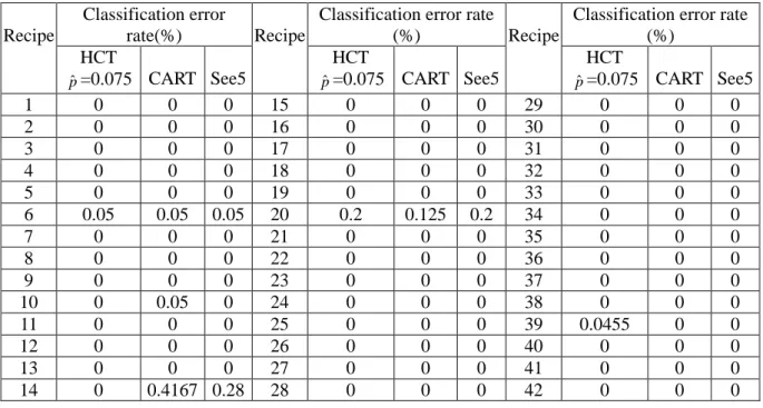
(39) table. From this table, we can calculate the sum of classification error rates of the proposed HCT with pˆ=0.075 is around 0.2955%; while the sum of classification error rates using See5 and CART are 0.53% and 0.6427%, which are 80% and 117% more than that of HCT, respectively. Thus HCT obtains a very successful classification result. Table 2.1. The units and related subsystems of the 12 attributes. Attribute k1 filament voltage k2 filament current k3 discharge voltage k4 discharge current k5 extraction electrode voltage k6 extraction electrode current k7 acceleration/deceleration voltage k8 magnetic field strength k9 high voltage power supply current k10 beam current k11 beam-line pressure k12 chamber pressure. k8. Unit Subsystem Volts ion source Amps ion source Volts ion source Amps ion source KV extractor mA extractor KV extractor KGauss mass analysis A mass analysis mA mass analysis Torr/e6 accelerator Torr/e6 accelerator. TC1 (2,3,4,9,10, 11,18,19,20,21, 37,38,39,40,41). k9. Cr0 (1~42). k8. Cr1 (8,14,15,16, 23,24,25,26,27, 28,29,30,31,32, 33,34,35). k9. k10 k8. Figure 2.10.. Cr2 (1,5,6,7,12, 13,17,22,36,42). k10. TC2 (23) TC3 (8,14,15,16, 24,25,26,27,28 ,29,30,31,32,3 3,34,35). TC4 (1,6,7,12,13). TC5 (5,17,22,36, 42). The clustering tree of the 42-recipe case.. 30.

(40) Table 2.2. The 10-fold cross validation classification error rate of the 42-recipe case.. Recipe. 1 2 3 4 5 6 7 8 9 10 11 12 13 14. Classification error Classification error rate Classification error rate rate(%) Recipe (%) Recipe (%) HCT HCT HCT pˆ=0.075 CART See5 pˆ=0.075 CART See5 pˆ=0.075 CART See5 0 0 0 15 0 0 0 29 0 0 0 0 0 0 16 0 0 0 30 0 0 0 0 0 0 17 0 0 0 31 0 0 0 0 0 0 18 0 0 0 32 0 0 0 0 0 0 19 0 0 0 33 0 0 0 0.05 0.05 0.05 20 0.2 0.125 0.2 34 0 0 0 0 0 0 21 0 0 0 35 0 0 0 0 0 0 22 0 0 0 36 0 0 0 0 0 0 23 0 0 0 37 0 0 0 0 0.05 0 24 0 0 0 38 0 0 0 0 0 0 25 0 0 0 39 0.0455 0 0 0 0 0 26 0 0 0 40 0 0 0 0 0 0 27 0 0 0 41 0 0 0 0 0.4167 0.28 28 0 0 0 42 0 0 0. Remark 1: From the test results shown in Table 2.2, we see that the superiority of HCT over CART and See5 is mostly due to the zero classification errors of recipe 14. What causes the classification errors of recipe 14 in CART or See5 is the overlapping of the attribute data between recipes 14 and 20. Thus, some test data patterns of recipe 14 may be classified to be recipe 20 in CART or See5. Fortunately, in HCT, recipe 14 and 20 have been classified into different TCs as can be observed from Figure 2.10. This drastically reduces the possibility of classifying recipe 14 to be 20. However, in HCT, recipe 20 may still be classified into recipe 14, which can also be observed from Table 2.3 for misclassification rate. Excluding recipe 14 from the data set, we repeat the complete training and test process, and the results show that the sum of classification error rates of HCT, CART, and See5 are 0.173, 0.248 and 0.182, respectively. Indeed the three sums of classification errors are closer, however, HCT is still the best among them. Furthermore, we also apply the three classifiers to the 26-recipe case that we mentioned at the beginning of this subsection, and the sum of classification error rates of HCT, CART and See5 are 0.225, 0.577 and 0.405, respectively.. 31.