基於攻擊圖形的混合式無線網路風險評估方法

(1)

國

立

交

通

大

學

電機與控制工程學系

碩

士

論

文

基於攻擊圖形的混合式無線網路風險評估方法

A Hybrid Approach for Attack Graph-Based Risk Assessment of

Wireless Networks

研究生：鍾興龍

指導教授：黃育綸博士

(2)

基於攻擊圖形的混合式無線網路風險評估方法

A Hybrid Approach for Attack Graph-Based Risk Assessment of

Wireless Networks

研究生：鍾興龍 Student：Hsing-Lung Chung

指導教授：黃育綸博士 Advisor：Dr. Yu-Lun Huang

國立交通大學

電機與控制工程學系

碩士論文

A Thesis

Submitted to Department of Electrical and Control Engineering College of Electrical and Computer Engineering

National Chiao Tung University in partial Fulfillment of the Requirements

for the Degree of Master

in

Electrical and Control Engineering

July 2007

Hsinchu, Taiwan, Republic of China

(3)

基於攻擊圖形的混合式無線網路風險評估

方法

學生：鍾興龍指導教授：黃育綸博士

國立交通大學電機與控制工程學系（研究所）碩士班

摘要

無線網路風險評估是無線安全領域中的關鍵技術之一。為了幫助管理者評估網路之安全程度，攻擊圖形以圖形化的表示方式來呈現分析結果，提供管理者在決策時的參考依據。近年來，許多學者利用層級程序分析法(Analytic Hierarchy Process Method，AHP) 及模糊語意量測法(Fuzzy Linguistic Measure method)來處理風險評估的問題，其網路評

估架構以3 層為主，然而此架構並不能表示各種網路配置資訊對不同類型無線網路攻擊所造成的影響，再者，層級程序分析法適用在不隨環境變動的評估項與評估法則間建立判斷矩陣，對於會隨環境變動的評估項，其擴充性較差；模糊語意量測法較難從模糊集合中取得量化數值，無法提供精確的分析結果。因此，我們結合層級程序分析法及模糊語意量測法並加以改良，提出一套分析無線網路安全性的風險評估模型。在此模型中，我們定義了一個 4 階層的無線網路風險評估架構，從此架構中，我們透過分析法則來求得每個配置資訊在不同網路攻擊類型中的影響程度，並使用模糊權重平均法(Fuzzy Weight Average Method，FWA)來計算各攻擊類型的模糊平均集合；為了能夠取得各個攻擊類型數值化的風險等級，我們設計一個量化方法從模糊平均集合求得量化數值。之後便可結合層級程序分析法，以所定義的專家經驗為基礎來計算風險值。最後，我們利用兩個無線網路上常見的拓樸為範例，證明此風險評估模型的有效性與實用性並利用圖形

(4)

A Hybrid Approach Attack Graph-Based Risk

Assessment of Wireless Networks

Student: Hsing-Long Chung Advisor: Dr. Yu-Lun Huang

Department of Electrical and Control Engineering

National Chiao Tung University

Abstract

Risk assessment of wireless networks is one of the crucial techniques in the area of wireless network security. A graph-based representation, called attack graph, has been developed to appear analytic results and support policies for administrators. Recently, the analytic hierarchy process (AHP) method and the fuzzy linguistic measure method have been applied to deal with risk assessment problems. The assessment architecture is based on 3 layers. However, the architecture can not represent influence of configurations on different attack types. In addition, the AHP method is hardly constructed judge matrixes if analysis items changed with network environment while the fuzzy linguistic measure method is hardly acquire quantifiable value from fuzzy set. Hence, we modify and combine the two methods to establish a new risk assessment model to analyze the security robustness of wireless networks. In the proposed model, we redefine 4-layer assessment architecture of wireless networks. From this architecture, we can obtain influential level of each configuration on different attack types through analysis rules and use the fuzzy weight average (FWA) method to calculate average fuzzy set of each attack type. In order to gather quantitative risk rating of each attack type, a quantitative method is designed to obtain value of average fuzzy set. Afterward the AHP method is applied to compute the risk value based on expert experience. Finally, two case studies are given to demonstrate validity and feasibility for risk assessment according to the proposed model. We also use the Graphviz tool to generate their attack graphs to describe the security robustness of these two examples.

(5)

誌謝

兩年的碩士班求學過程，要感謝的人很多。特別要感謝指導教授黃育綸老師，兩年來細心的指導與關懷，除使得本論文得以順利完成之外，也讓我學習到做人做事的道理，使我受益良多，在此表示由衷的謝意。在研究的過程中，您不時的給予我在想法上的啟發，也在我遇到困難與挫折時，竭盡所能的給予我最大的幫助與鼓勵，並時時刻刻注意學生在研究上的進度，適度的給予糾正及調整研究的方向，使得我能夠有繼續研究的動力。同時，也要感謝謝續平教授、曾文貴教授、以及何福軒博士，在口試期間提出的寶貴意見與指正，使我可以了解論文不足的地方，並對此進行改善，使得本論文更加完整。其次，感謝「即時嵌入式系統實驗室」的黃詠文學長以及蔡欣宜學姐在論文上的指導；也感謝其餘實驗室的成員在學業上的切磋，透過彼此間腦力激盪，使得我的觀念更加的清晰並啟發更多的想法，此外實驗室閒暇之餘的娛樂活動，讓我能夠在身心愉悅的情況下持續我的研究，增加我對實驗室的向心力；也感謝其他交大的師長、同學、朋友們，在學習道路上的指引與陪伴，透過彼此的專長來合力完成許多專案計畫，增加我在專案計畫上的經驗；感謝大學時期的同學，在生活及研究上給我的幫助，像是在研究上的經驗以及生活資訊的提供，使我獲益良多。除此之外，特別要感謝辛苦扶養我長大的父親、母親，還有我的妹妹，不論是在生活上及精神上，都是我最重要的支柱，由於你們的關愛與支持，讓我無後顧之憂，也才有今天的我。最後，向在我人生道路上，一路陪伴我走來的所有人們，獻上最誠摯的祝福與感謝。

(6)

List of Tables

Table 1. Classification of Access Control Attack ...14

Table 2. Classification of Monitor Attack ...15

Table 3. Classification of DoS/ DDoS attack ...15

Table 4. Classification of AP Key Crack ...16

Table 5. Classification of Remote Login ...16

Table 6. Classification of Virus and Backdoor ...17

Table 7. The Risk Factors of Each Rule ...28

Table 8. Risk Degree and Risk Weight of Probability...28

Table 9. Risk Degree and Risk Weight of Impact Severity ...29

Table 10. Risk Degree and Risk Weight of Uncontrollability ...29

Table 11. A Nine-Member Linguistic Term Set...29

Table 12. Linguistic Term for Access Level of Attacker ...30

Table 13. Linguistic Term for Data Encryption of Running Service...30

Table 14. Safety of Encrypted Type ...31

Table 15. Probability of Gather Configurations ...31

Table 16. Linguistic Term for Safety and Acquirable Probability of Configuration ...32

Table 17. Linguistic Term for Risk Level of Configuration...32

Table 18. Linguistic List of the Weight and the Risk Level (AP1 and STA1) ...38

Table 19. Risk Level of Total Risk Value ...41

(9)

List of Figures

Fig. 1. Layer Encryption (Welch et al. [4]) ...2

Fig. 2. Risk Assessment Methodology Flowchart (Gray et al. [26])...8

Fig. 3. The Hierarchy Structure of Risk Assessment (Zhao et al. [27], [28])...9

Fig. 4. Fuzzy Weight Average (FWA) Architecture (Liao et al. [27], [28]) ... 11

Fig. 5. The Assessment Architecture of the Wireless Networks...13

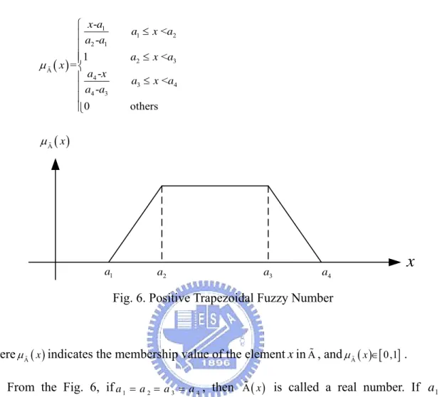
Fig. 6. Positive Trapezoidal Fuzzy Number ...18

Fig. 7.Wireless Network Example (AP and station)...27

Fig. 8. Attack Graph with AP1 and STA1 ...42

Fig. 9. Wireless Network Example (AP and two stations) ...43

(10)

Chapter 1 Introduction

In today’s society, wireless networks bring great convenience to network users, and also brings a large collection of threats into wireless environment. For this reason, a risk assessment model in design of wireless networks has become a popular issue in order to deal with security problems. Furthermore, the attack graph is proposed to display the results of risk assessment. The first chapter of this thesis is organized in to three sub sections: Section 1.1 presents the background of this research. Our contribution is presents in section 1.2, and the remainder of the thesis is introduced in section 1.3.

1.1 Background

Wireless networks have become the most interesting target for attackers because they use airwave instead of physical medium to interconnect wireless devices or stations. Several papers have published some specific threats to wireless networks. In [1], the researchers pointed out the weaknesses in WEP encryption. One of the main vulnerabilities in WEP is that the uses of a 32-bit CRC checksum and a 24-bit Initialization Vector (IV) for the encryption algorithm. The CRC checksum was intended to detect unintentional errors in the packet. Attackers could still modify the packet and calculate a new CRC checksum to make it look the unmodified. The problem with the 24-bit IVs was that the IVs were too few to guarantee only use at one time. Attackers will see enough traffic to completely exhaust the entire domain of the 24-bit IVs, and then they could see two encrypted packets with the same IVs to crack the encryption key. In addition, the RC4 algorithm had less security because of the weak key [2]. The problems of WEP have been improved by WPA, but Lehembre [3] mentioned the

(11)

most practical vulnerability was WPA’s PSK key. The key could be obtained through dictionary attack. Some wireless attacks including eavesdropping attack, man in the middle attack, access attack, DoS attack and DDoS attack, were illustrated in [4]-[7]. Attackers will utilize some important information from wireless packets. From [4], Welch et al. presented the encrypted tunnels of network layer and data link layer as explained in Fig. 1. Hence attackers can identify the source and destination MAC address when layer 2 is employed. Layer 3 encryption let the IP address of sender and receiver open for viewing.

Fig. 1. Layer Encryption (Welch et al. [4])

Nowadays, administrators can use a lot of tools find the security holes of each host that may cause attacks. In order to defend attacks efficiently, a graphical environment is needed for security issues. Attack graph is a graphical representation and has focused on security analysis. At first it is used to appear the vulnerabilities of the host. As the development of network, the attack graph not only displays the vulnerabilities among the network, but also describes the attack behavior of attackers. After that some researchers use attack graph to

(12)

analyze the safety of the network environment according to the network configurations. Altogether, the arrack graph provides a view to help administrators understand where the security problems are and support them to make the environment more robust.

Attack graphs have traditionally been constructed manually by administrators [8]. But more recently, the network environment becomes more and more vast and complex. Constructing attack graphs by the hand is impractical and tedious. Thus, significant progress has been made to generate attack graph automatically [9]-[16].

The development of attack graph includes vulnerability description [9]-[16], risk assessment [17], reliability analysis [18] etc. The way to enhance the network security before being attacked is risk assessment.

The advantages of network security risk assessment are as follows: (1)Monitoring critical information and protecting the network environment more effectively;(2)Supporting the security policies quickly for decision maker;(3)Providing useful information for administrators [19]-[21].

There are several risk assessment methods, such as cause-consequence tree analysis and fault tree analysis, etc. The methods usually use mathematical or statistical techniques to evaluate risk values [22]. However, these methods are not suitable for wireless network security risk analysis because the security issues focus on environment of wireless networks. Recently, we know risk analysis can be analyzed through linguistics method or analytic hierarchy process (AHP) method, but there are some drawbacks of the two methods. These issues we will discuss later.

The purpose of this thesis is to establish an assessment model. The model contains an extendable assessment architecture and a risk analysis method for quantitative value of wireless network security. We then use tool to produce attack graph for wireless network analysis. The nodes and edges of attack graphs denote wireless device and risk value between two nodes, respectively. Hence administrators can easily understand the security robustness of

(13)

WLAN.

1.2 Contribution

A major advance of the assessment architecture in this thesis over other risk assessment architectures is that it considers the configurations of wireless networks. It is more flexible than the exiting architectures due to the fact that some configurations of each node will be changed at any moment by the users. Furthermore, the risk assessment method, which combines the AHP method and the linguistics of the fuzzy measure method, is applied to the risk assessment. The approaches can objectively determine the judge matrixes and the risk weight of risk factors based on the expert experiment. Afterward the total risk value can be calculated through matrix operation.

1.3 Synopsis

The rest of this thesis is organized as follow. In Chapter 2, we review related work in this area. In Chapter 3, we propose new hierarchical risk assessment architecture and risk analysis method for wireless network security. Chapter 4 gives 2 examples to illustrate the proposed architecture is useful to network risk assessment. In addition, we provide a view of attack graph based on the configurations of WLAN. Finally, Chapter 5 presents some conclusions.

(14)

Chapter 2 Related Work

Wireless networks have many security holes that may cause attacks and attackers always use these holes to achieve their goals. In order to keep attackers from accessing, monitoring and modifying network packets, some security tools can help to detect the configurations information of wireless networks. Furthermore, the administrators can use the configurations for risk assessment and show the risk value in the graph. These graphs collect the crucial information to aid network administrators in efficiently reinforcing network security. In this chapter, we first review the past researches for attack graph. Section 2.2 specifies the process of risk assessment. The risk assessment approaches of network are reviewed in section 2.3.

2.1 Past Researches for Attack Graph

Attack graphs have been widely used in security issues. Any attack or vulnerability could be observed from the path which went from an initial node to a success node. Formerly, the attack graph in which each node represented a state of attackers, and each edge represented an atomic attack that changed the state. Initial nodes expressed the states that attackers had not conducted any atomic attack, and success nodes expressed the states that attackers had successfully reached his goal [10]. Such the attack graph became very complex if the network added more hosts. As a result, an automatic tool is useful for administrators to establish the attack graph.

Many methods have been proposed to define the attack graph and automatically construct it. Ortalo et al. [9] developed a method named privilege graph, the nodes in privilege graph represented privileges owned by the users and the edges represented

(15)

vulnerabilities that would change privileges. The graph displayed different ways that attackers could reach his goal. From [10], Philips and Swiler defined an attack graph which was generated by three types of input: attack templates, configurations file, and attacker profiles. Attack templates represented the necessary information or the steps of attack. The configuration file saved the detail information that attackers wanted, and the capabilities of attackers were stored in attacker profiles. In [11], Swiler et al. implements the method of [10] into a tool. Moreover, the elimination of redundant paths was also surmounted. Ammann et al. [12] developed a graph-based algorithm which was capable of finding mostly vulnerabilities. Ingols et al. [13] defined another attack graph which called MP attack graph. The graph where the nodes were classified three types. State nodes presented access levels of attackers on the hosts. Prerequisite nodes represented reachable hosts from state nodes. Vulnerability nodes presented vulnerabilities on the specific services.

More recently, Jha and Wing [18] proposed the attack graph to consider the network environment included the network user, IP address, running service, etc. In [8], [23]. Sheyner

et al. defined the attack graph where each node denoted a state of the network systems and

each edge denoted an atomic attack which changed state. They also added three configurations included system open port numbers, connection relations and vulnerabilities into the configuration file and used model checking tool called “NuSMV” [24] to analyze attack graph. Zhang et al. [14] expended the privilege into the attack graph and compared with [8]. The result proved that their graph was much simpler than that in [8]. The reason was that the model checking tool is not able to determine the privilege of the network system. From [15], Noel et al. defined another attack graph of network environment. Each node represented the machine on network and each edge represented the vulnerabilities that attackers used to compromise the network machine. Instead, the network machines were distributed to several subnets and then utilize the graph-drawing tool [25] to generate attack graph. This provided the good views for the administrators to know which subnets were easily

(16)

attacked. An architecture was proposed by Kotenko and Stepashkin [16] for security analysis based on construction of attack graph. In addition, they evaluated the network risk according to different wire network environment. Hence the attack graph not only to describe the vulnerabilities of the system but also to defend the environment of network before being attacked by attackers.

2.2 The Process of Risk Assessment

Risk assessment indicates the risks to network security and determines the probability of occurrence. Although it is impossible to use the risk assessment to eliminate all risks, administrators may expect the risks be reduced and adjust the configurations of the network environment.

According to [26], Gray et al. proposed the risk assessment process. The process was decomposed into nine parts and the flowchart is shown in Fig. 2.

z System characterization – In this step, the analysis items are identified, along with the

configuration information and risk classifications that constitute the assessment model.

z Threat identification – The attacks of assessment environment are described in this step. z Vulnerability identification – The goal of this step is to list the vulnerabilities that could

be exploited by attackers.

z Control analysis – In this step, the rules is defined to describe the controllability or

uncontrollability of the system after being attacked.

z Likelihood determination – The rules is defined to describe the probability of launching

attacks.

z Impact analysis – In this step, the rules is defined to describe the impact severity of the

system after being attacked.

(17)

z Control recommendations – The goal of the recommended controls is to notice the

security risks and support the experts to reduce the risks.

z Results documentations – Once the risk assessment has been completed, the results

should be documented to help administrators understand the risks.

(18)

2.3 The Approaches of Risk Assessment

Fig. 3. The Hierarchy Structure of Risk Assessment (Zhao et al. [27], [28])

In [27], [28]. Zhao et al. designed a risk assessment architecture which depended on Gray’s process as shown in Fig. 3. The top layer was the total risk value of network; the rules were defined in second layer and the network attacks were defined in the lowest layer. They also recommended a risk assessment method, which combined analytic hierarchy process (AHP) method and matrix operation for risk assessment. The steps of AHP method were specified as follow: (1) Constructing the hierarchy structure for risk assessment; (2) Constructing the judge matrix by expert experience; (3) Determining the weights of risk factors of each rule; (4) Calculating the quantitative coefficients depends on judge matrix. After finished the first three steps, they estimated the unknown probabilities of risk factors of each attack type, p1, p2, …, pm, by using the Shannon entropy function [29] - [30]. This

function was put forward to decide the weight of each network attack, as follows:

1 ln 1 = - m ln m i i i H p p =

∑

(1)

(19)

The judge matrix R of a rule is obtained by experts’ experiences as well as a corresponding vector b, which represents weights of risk factors of the rule. Suppose that R is an n-by-m matrix in which n implies there are n attack types in the wireless environment, and m represents the number of the risk factors in the rule.

11 12 1 21 22 2 1 2 m m n n nm r r r r r r R r r r ⎡ ⎤ ⎢ ⎥ ⎢ ⎥ =_⎢ _⎥ ⎢ ⎥ ⎢ ⎥ ⎣ ⎦ b = [b1, b2,…, bm]T

The weight vector, qT_{, is also acquired from the matrix by using Eq. (1).}

q = [q1, q2,…, qn]T

Then the risk value of each rule can be calculated by the following equation:

T 1 1 = n q_j m _jk _k j k r R r = = ⎛ ⎞ = ⋅ ⋅ _⎜ _⎟ ⎝ ⎠

∑ ∑

q b b (2)

Changguang et al. [31] redesigned the architecture for wireless networks and used the same risk assessment method as [28]. They defined that the total risk value is the function of risk probability, impact severity and uncontrollability. The probability is denoted as p, the impact severity is denoted as c and uncontrollability is denoted as u, the risk happened denoted as s, whereas denoted as t. Then the formulas of total risk value can be calculated as:

(

)

(

)( )( )

=1-1- =1-1- 1- 1-= + + - - - -t -t t s s s s s s s s s s s s s s s

R= f risk probability, impact severity ,uncontrollable p c u

p c u

p c u p c p u c u p c u

= (3)

In [32], we know risk analysis could be analyzed through fuzzy linguistics; the information about risk was calculated via the fuzzy set theory and expressed in a natural language. However, the main drawback of the method is that it can not correctly calculate the average fuzzy set between two fuzzy sets. Therefore, Chen et al. [33] proposed an analysis method, which is called the center-of-gravity (COG) similarity method, to overcome the drawback of [32]. If the fuzzy value is not between zero and one, it is translated into the standardized fuzzy set. The average fuzzy set can be calculated by using fuzzy weight average (FWA) method shown as follows:

(20)

n =1 n =1 = i i i i i W R R W ×

∑

(4)

Where Ris the average fuzzy set of the system security, W_iandR_iare the weight and the

security risk level of each subsystem, respectively.

Liao et al. [34] proposed a hierarchical structure to construct the risk assessment architecture and used FWA method to compute the total risk value. The hierarchical structure was shown in Fig. 4, where each edge denoted fuzzy risk level and each node denoted weight importance of subsystem, respectively.

Fig. 4. Fuzzy Weight Average (FWA) Architecture (Liao et al. [27], [28])

The AHP method could easily obtain the quantitative value, but hardly constructed the judge matrixes if the analysis items changed with the environment. On the contrary, the linguistics method could easily extend the architecture, but hardly acquire the quantitative values.

(21)

Chapter 3 The Proposed Model for Risk Assessment

In this chapter, the proposed model is presented for risk assessment. In section 3.1, a hierarchical risk assessment architecture which combines the fuzzy linguistics and numerical descriptions is proposed to analyze the security robustness of wireless networks. Section 3.2 introduces the details of the attack types that we construct from the assessment architecture. In order to integrate fuzzy linguistics with numerical descriptions and calculate the risk value successfully, some definitions are described in section 3.3.

3.1 Constructing the Risk Assessment Architecture

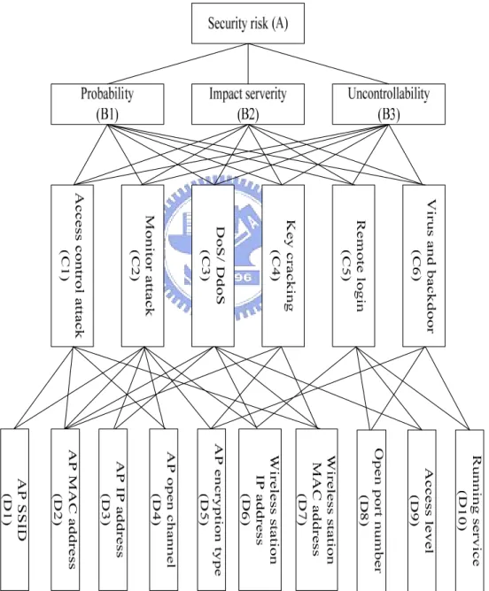
According to the AHP method [26], [28], [32], the first step is to construct the risk assessment architecture of wireless networks. We can utilize layer structures to decompose complexity relationships into simple relationships. The highest layer is the goal, which is the total risk value of wireless environment. The second layer defines the same rule as [28]. The rule is judged in the aspects of probability of suffering attacked, impact severity and uncontrollability after being attacked. The third layer classifies the wireless attack types into six dimensions. Configurations in the lowest layer are the categories for wireless attack types that attackers will use when attacks occur. Fig. 5 shows the hierarchy risk assessment architecture of wireless networks.

As for the relationships among the architecture, we explain from the fourth layer to the top layer. The subcomponents of the fourth layer are represented by fuzzy linguistics which means the security weights of configurations and each edge is denoted the risk level between the configuration and the attack type. And then, the average fuzzy set of each attack type can be calculated through FWA method. By the expert experience, the risk degree between the

(22)

rules and the attack types can be decided. Hence we need to find the way to integrate fuzzy set and numerical value. In addition, according to [29], [30], the weights of attack types denote the discrepancies of experts. Hence we don’t need to consider the influence of configurations, and we only need to use risk degrees to decide weights of attack types. By using Eq. (1), the weights of attack types can be calculated through these degrees.

Fig. 5. The Assessment Architecture of the Wireless Networks

In order to combine fuzzy set with numerical value, the average fuzzy set should be quantified and then execute multiplication to the risk degree. The quantitative values of attack

(23)

types are called risk ratings. Attackers will get higher risk rating if they acquire more configurations. If we acquire quantitative risk ratings of n attack types, a1, a2, ..., an, the judge

matrix can be modified where each row denotes the attack type and each column denotes the risk factor of the rule.

1 11 1 12 1 1 2 21 2 22 2 2 ' 1 2 m m n n n n n nm a r a r a r a r a r a r R a r a r a r ⎡ ⎤ ⎢ ⎥ ⎢ ⎥ =_⎢ _⎥ ⎢ ⎥ ⎢ ⎥ ⎣ ⎦

Afterward the risk value of each rule can be modified as ' 1 1 n m j j jk k j k r α r = = ⎛ ⎞ = ⎜_⎜ ⎟_⎟ ⎝ ⎠

∑ ∑

q b (5)

Finally, according to Eq. (3), the total risk value can be calculated by matrix operations.

3.2 Classification of Attack Types

By the third layer of the risk assessment architecture, it classifies the attack types of wireless networks mainly include the following portions:

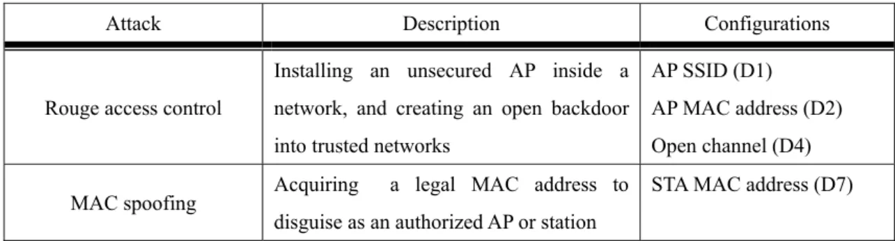
3.2.1 Access Control Attack

These attacks attempt to utilize the wireless resources which are not permitted by administrators. The description and the configurations of these attacks are shown in Table 1.

Table 1. Classification of Access Control Attack

Attack Description Configurations

Rouge access control

Installing an unsecured AP inside a network, and creating an open backdoor into trusted networks

AP SSID (D1) AP MAC address (D2) Open channel (D4) MAC spoofing Acquiring a legal MAC address to

disguise as an authorized AP or station

STA MAC address (D7)

(24)

3.2.2 Monitor Attack

These attacks try to intercept aerial packets to obtain essential information concerned by attackers. The description and the configurations of these attacks are shown in Table 2.

Table 2. Classification of Monitor Attack

Eavesdropping

Capturing and decoding unprotected packets to obtain potentially sensitive information AP IP address (D3), Encryption type (D5) STA IP address (D6) Evil Twin AP Masquerading as an authorized AP by beaconing the wireless service set identifier to lure users

AP SSID (D1) AP MAC address (D2) Open channel (D4)

Man in the Middle

Masquerading as an authorized AP and STA at one time, and collecting the packers between them

AP IP address (D3) Encryption type (D5) STA IP address (D6)

3.2.3 DoS/ DDoS Attack

These attacks are incidents which wireless stations and access points are interdicted of the services of the resource. The description and the configurations of these attacks are shown in Table 3.

Table 3. Classification of DoS/ DDoS attack

Authentication flood

Sending the forged authentication packets from random MAC addresses to fill a target AP’s association table

AP MAC address (D2) STA MAC address (D7)

De-authentication flood

Flooding wireless stations by sending the forged de-authentication packets to disconnect users from an access point

AP MAC address (D2) STA MAC address (D7)

ICMP Ping Flood Using attack tools to send a large ICMP packets to a wireless station or APs

AP IP address (D3) STA IP address (D6)

(25)

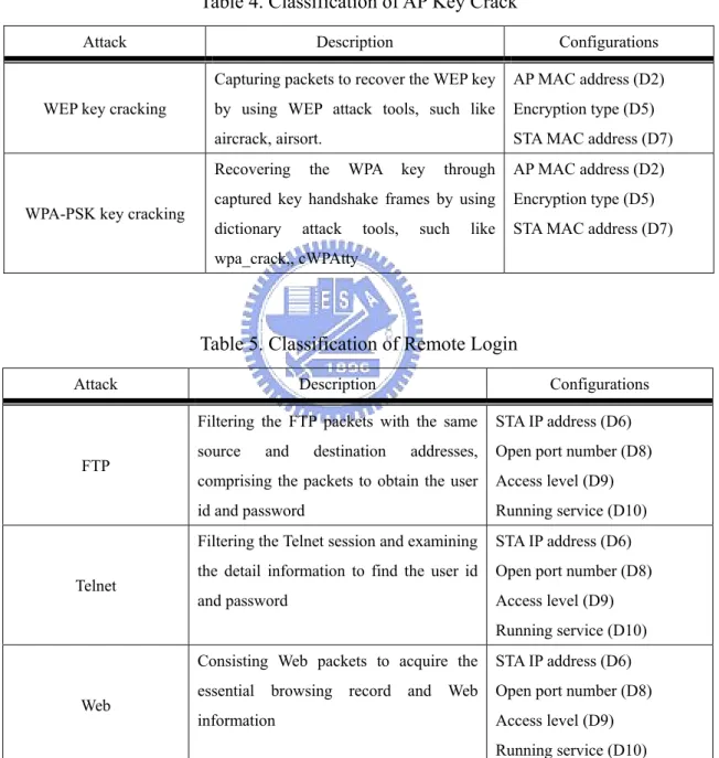
3.2.4 AP Key Cracking

These attacks try to decipher the encryption data to obtain the password which is configured by the access point. The description and the configurations of these attacks are shown in Table 4.

Table 4. Classification of AP Key Crack

WEP key cracking

Capturing packets to recover the WEP key by using WEP attack tools, such like aircrack, airsort.

AP MAC address (D2) Encryption type (D5) STA MAC address (D7)

WPA-PSK key cracking

Recovering the WPA key through captured key handshake frames by using dictionary attack tools, such like wpa_crack,, cWPAtty

AP MAC address (D2) Encryption type (D5) STA MAC address (D7)

Table 5. Classification of Remote Login

FTP

Filtering the FTP packets with the same source and destination addresses, comprising the packets to obtain the user id and password

STA IP address (D6) Open port number (D8) Access level (D9) Running service (D10)

Telnet

Filtering the Telnet session and examining the detail information to find the user id and password

Web

Consisting Web packets to acquire the essential browsing record and Web information

3.2.5 Remote Login

(26)

in order to connecting with the remote hosts. The description and the configurations of these attacks are shown in Table 5.

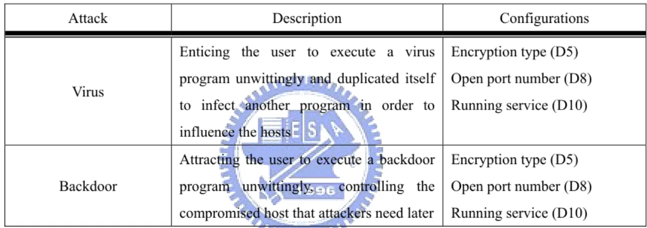
3.2.6 Virus and Backdoors

These attacks attempt to infect some files to influence the hosts or let them open some services that attackers need. The description and the configurations of these attacks are shown in Table 6.

Table 6. Classification of Virus and Backdoor

Virus

Enticing the user to execute a virus program unwittingly and duplicated itself to infect another program in order to influence the hosts

Encryption type (D5) Open port number (D8) Running service (D10)

Backdoor

Attracting the user to execute a backdoor program unwittingly, controlling the compromised host that attackers need later

Encryption type (D5) Open port number (D8) Running service (D10)

3.3 Definition

In this section, we first define the composition of the fuzzy set and their arithmetic operations for the purpose of the risk assessment architecture. Also, a quantitative method of the fuzzy set, which extends the discrete fuzzy set, is proposed to determine the value of risk rating to integrate with expert experience.

Definition 1. Positive trapezoidal fuzzy set. Suppose that a positive trapezoidal fuzzy set ( )

A x can be represented as(a a a a1, , ,2 3 4), where a a a1, ,2 3 and a4are real numbers, is described as any fuzzy subset with its membership function μ_A( )x is defined as follows and shown in

(27)

Fig. 6.

( )

A x μ 1 a a₂ a₃ a₄

( )

1 1 2 2 1 2 3 A 4 3 4 4 3 -< -1 < = < -0 others x a a x a a a a x a x a x a x a a a μ ⎧ _≤ ⎪ ⎪ ⎪ ≤ ⎪ ⎨ ⎪ _≤ ⎪ ⎪ ⎪⎩

x

Fig. 6. Positive Trapezoidal Fuzzy Number

Whereμ_A( )x indicates the membership value of the elementxinA, andμ_A( )x ∈

[ ]

0,1 .

From the Fig. 6, ifa₁ =a₂=a₃ =a₄, then A x( ) is called a real number. If a₁ = a₂

anda₃= , then a₄ A x( ) is called a crisp fuzzy set. Ifa₂ = , then a₃ A x( ) is called a triangular

fuzzy set.

Definition 2. Arithmetic operations of fuzzy sets. For the two positive trapezoidal fuzzy setsA x( ) andB x( ), where A( ) (x = a a a a1, , ,2 3 4)andB( ) (x = b b b b1, , ,2 3 4), the arithmetic operations can be defined as follows.

i) Addition:

(

) (

)

(

11 213 24 2 1 23 33 44 4

)

A + B , , , + , , , = + , , , a a a a b b b b a b a b a b a b = + + + (6) ii) Subtraction:

(

) (

)

(

11 2 43 24 3 1 23 23 44 1

)

A B , , , - , , , = , - , - , -a -a -a -a b b b b a b a b a b a b − = − (7)

(28)

iii) Multiplication:

(

)

(

)

(

)

(

)

(

)

1 1 1 4 4 1 4 4 2 2 2 3 3 2 3 3 2 2 2 3 3 2 3 3 1 1 1 4 4 1 4 4 1 1 2 2 3 3 4 4 A B min , , , , min , , , , max , , , , max , , , = , , , a b a b a b a b a b a b a b a b a b a b a b a b a b a b a b a b a b a b a b a b ⎡ × = ⎣ ⎤⎦ (8) iv) Division:

(

)

(

)

(

)

(

)

(

)

1 1 1 4 4 1 4 4 2 2 2 3 3 2 3 3 2 2 2 3 3 2 3 3 1 1 1 4 4 1 4 4 1 4 2 3 3 2 4 1 A / B min , , , , min , , , , max , , , , max , , , = a b ,a b ,a b ,a b a b a b a b a b a b a b a b a b a b a b a b a b a b a b a b a b ⎡ = ⎣ ⎤⎦ (9)

Definition 3. Quantification of a fuzzy set. For a bounded fuzzy set A x( ), f

(

A( )x

)

is defined as the risk rating which means the distinction between a given fuzzy set and its fuzzy complement. For the set is defined within the interval [0, 1], the quantification of the fuzzy set can be measured by:

( )

(

)

1 ( ) 0

A = 2A -1

f x

∫

x dx (10)

According to [35], Yager and Kirl introduced the fuzziness of the fuzz set A x( ) using the summation of the distinction which is measured by distance function between the fuzzy set and its fuzzy complement is defined as:

( )

(

)

(

( ) ( )

)

(

( )

(

( )

)

( ) c X X X A = A -A = A - 1-A = 2A -1 x x x f x x x x x x ∈ ∈ ∈

∑

(11)

Eq. (10) is suitable only to the discrete fuzzy set. However, the fuzzy set which is defined on the bounded fuzzy set can be readily modified. Consider the interval [0, 1]. The replacement results of Eq. (9) can be described in the following equation:

( )

(

)

( )

(

( )

)

( ) 1 0 1 0 A = A - 1-A = 2A -1 f x x x dx x dx

∫

□

(29)

Definition 4. Quantitative coefficient of the judge matrix. For each judge matrix, the quantification coefficient c , which is the certainty of each attack type is defined as: _j

1-j j

c = e (12)

where e is defined by Shannon’s entropy measure [36] based on Eq. (1). The entropy _j e is _j

the uncertainty of the given risk degrees and is defined as:

(

1 2

)

1 1 , , , - ln ln m j m j j j e S p p p p p m = = … =

∑

(13)

Definition 5. Normalized weight of the quantitative coefficient. For the normalized weightq , each quantification coefficient _k c should be equally preferred. The formula is _j defined as: 1 1 1-j k n j j j n j j c q c e e = = = =

∑

(14)

Definition 6. Scope of the total risk value. For the total risk valueR ,R∈

[ ]

0,1 , implies that

the larger risk value reaches, the more danger of the wireless environment.

3.4 General Solution Algorithm

Our process of risk assessment is now almost complete, all that remains is to describe the calculating procedures with the steps in the analysis of wireless networks. In the following, we make some assumptions and then design a solution algorithm for risk assessment of wireless networks.

(30)

(1) We construct an m × n matrix to represent the configurations that the attack types utilize to start the attack. The rows denote the configurations and the columns denote the attack types. The matrix C is 11 12 1 21 22 2 1 2 n n m m mn c c c c c c C c c c ⎡ ⎤ ⎢ ⎥ ⎢ ⎥ = ⎢ ⎥ ⎢ ⎥ ⎣ ⎦

Remark. The matrix is boolean. If cij =1, it means that the jth attack type needs the ith

configuration; whereas the jth attack type doesn’t need the ith configuration.

(2) Suppose that the experts define a fuzzy linguistic representation vectors MF = [mf1,

mf2, …, mfk] of k elements, where each element includes four membership values.

(3) Suppose that the experts define a fuzzy risk levels vector L = [l1, l2,…, lm] of m elements

of the configurations, where each element includes four membership values.

(4) Suppose that there exists a vector Rv = [rv1, rv2,…, rvk], where the ith element denotes an

n × qi matrix. The rows represent the attack types and the columns represent the risk factors of

each rule that defined by the experts.

(5) Suppose that there exists a vector Bv = [bv1, bv2,…, bvk], where each element denotes a

vector which means the weights of the risk factors that defined by experts. And the size of the

ith element is qi.

The general solution algorithm is shown as follows:

Algorithm 3.1 Generalized Version for Risk Value Calculation Input: A configuration file, config_file;

A m × n matrix C;

A risk level vector L of configurations of size m;

A vector RV of size r, of which the ith element is an n × qi matrix

A vector BV of size r; of which the ith element is a vector of size qi

Output: Risk value

Risk-Value-Calculate(config_file, C, L, RV, BV)

(31)

2 Let W be an array of size n

3 Set the weight value of each element of W according to the configurations and user’s rules

4 Let RC be an array of size n

5 for i ← 1 to n 6 do mul ← 0 7 sum ← 0 8 for j ← 1 to m

9 do if C[j, i ] = 1 ► Check if the jth_{configuration is used by the}

ith_{attack type}

10 then mul ← mul + W[j ]．L[j ] 11 sum ← sum + W[j ]

12 RC[i ] ← mul/ sum

13 let F be an array of size n

14 for i ← 1 to n

15 do F[i ] ← integrate |(2RC[i ])-1| from 0 to 1

16 let cV be a vector of size r, of which the element is a vector of size n

17 let qV be a vector of size r, of which the element is a vector of size n

18 for i ← 1 to r 19 do R ← RV[i ] 20 c ← cV[i ] 21 q ← qV[i ] 22 sum ← 0 23 for j ← 1 to n 24 do e ← 0 25 for k ← 1 to columns[R] 26 do R[j, k] ← F[j ]．R[j, k] 27 e ← e + (R[j, k]/ F[j ])．ln (R[j, k]/ F[j ]) 28 e ← -e / ln columns[R] 29 c[j ] ← 1 - e 30 sum ← sum + c[j ] 31 for j ← 1 to n 32 do q[j ] ← c[j ] / sum 33 Let Rr be a vector of size r

34 for i ← 1 to r

35 do Rr[i ] ← qV[i ]T RV[i ] bV[i ]

36 use the risk value of each rule, Rr[i ], to calculate the total risk value, risk 37 return risk

(32)

Suppose that experts define three rules, probability before being attacked (ps), impact

severity after being attacked (is) and system uncontrollability after being attacked (us), to

determine the total risk of a system. There are w risk factors of probability, x risk factors of impact severity, and y risk factors of uncontrollability. If there are n attack types of assessment architecture, then the proposed approach has the following property.

Property: if an attacker obtains more information of the environment E1 than that of the

environment E2, then the risk existing in E1 is larger than that in E2.

Proof.

If an attacker obtains more configurations of the wireless environment E1 than that of E2, according to experts’ experience, E1’s rating vector, α, is indeed larger than E2’s rating vector, α’, where

1, 2, , n

α= ⎡_⎣α α α ⎤_⎦T ,α'= ⎡⎣α α' , ' , , '1 2 αn⎤⎦

T_.

Assume that without loss of generality that αi > αi’ and all the other rating elements in α and

α’, are the same, i.e. αj = αj’ ∀j = 1, 2, 3, … ,n and j ≠ i.

By the definitions and algorithm steps introduced in Chapter 3, three judge matrixes, Rp,

Ri, and Ru, are obtained by experts’ experiences as well as the corresponding vectors, bp, bi and bu, which represent weights of risk factors of the three rules.

11 12 1 21 22 2 1 2 w w p n n nw r r r r r r R r r r ⎡ ⎤ ⎢ ⎥ ⎢ ⎥ = ⎢ ⎥ ⎢ ⎥ ⎢ ⎥ ⎣ ⎦ 11 12 1 21 22 2 1 2 x x i n n nx r r r r r r R r r r ⎡ ⎤ ⎢ ⎥ ⎢ ⎥ =_⎢ _⎥ ⎢ ⎥ ⎢ ⎥ ⎣ ⎦ 11 12 1 21 22 2 1 2 y y u n n ny r r r r r r R r r r ⎡ ⎤ ⎢ ⎥ ⎢ ⎥ = ⎢ ⎥ ⎢ ⎥ ⎢ ⎥ ⎣ ⎦ bp = [bp1, bp2,…, bpw]T, bi = [bi1, bi2,…, bix]T, and bu = [bu1, bu2,…, buy]T. Three weight vectors, cpT, ciT, and cuT, are also acquired from the matrixes, where cp= [cp1, cp2,…, cpn] T, ci= [ci1, ci2,…, cin] T, and cu= [cu1, cu2,…, cun] T, 1 p _ln 1 c 1 q ln w j jk jk k r r − = ⎛ ⎞ = −_⎜ ∑ _⎟ ⎝ ⎠, 0 c≤ p j ≤1 1 i _ln 1 c 1 s ln x j jk jk k r r − = ⎛ ⎞ = −_⎜ ∑ _⎟ ⎝ ⎠, 0 c≤ i j ≤1

(33)

1 u _ln 1 c 1 t ln y j jk jk k r r − = ⎛ ⎞ = −_⎜ ∑ _⎟ ⎝ ⎠, 0 c≤ u j ≤1

Then we can obtain three normalized weight vectors, qpT, qiT, and quT, where qp= [qp1, qp2,…, qpn] T, qi= [qi1, qi2,…, qin] T, and qu= [qu1, qu2,…, qun] T, p p p 1 q j j n j j c c = =

∑

, 0 q≤ p j≤1 i i i 1 q j j n j j c c = =

∑

, 0≤qi j ≤1 u u u 1 q j j n j j c c = =

∑

, 0 q≤ u j ≤1

Given the above vectors and matrixes, in the environment E1, ps (the probability of

suffering attacked), is (the impact severity after being attacked) and cs (the uncontrollability

after being attacked) are determined.

1 1 n w s j j jk j k p α r = = ⎛ ⎞ = ⎜_⎜ ⎟_⎟ ⎝ ⎠

∑ ∑

qp bpk , 0≤ps≤1 i 1 1 q b n x s j j jk k j k i α r = = ⎛ ⎞ = ⎜_⎜ ⎟_⎟ ⎝ ⎠

∑

i

∑

, 0≤is ≤1 u 1 1 q b y n s j j jk k j k u α r = = ⎛ ⎞ ⎜ ⎟ = ⎜ ⎟ ⎝ ⎠

∑

u

∑

, 0≤us ≤1

Similarly, the three corresponding values of the environment E2 are determined.

p 1 1 ' q ' b n w s j j jk k j k p r = = ⎛ ⎞ = ⎜_⎜ α ⎟_⎟ ⎝ ⎠

∑ ∑

p , 0≤ p's≤1 i 1 1 ' q ' b n x s j j jk k j k i α r = = ⎛ ⎞ = ⎜_⎜ ⎟_⎟ ⎝ ⎠

∑

i

∑

, 0 ≤i's ≤1 u 1 1 ' q ' b y n s j j jk k j k u α r = = ⎛ ⎞ ⎜ ⎟ = _⎜ _⎟ ⎝ ⎠

∑

u

∑

, 0≤u's ≤1

(34)

Finally, by Eq. (3), we can get R and R’, the total risks existing in the environment E1 and E2, respectively.

R=1-(1-ps)* (1-is)* (1-us), and R’=1-(1-ps’)*(1-is’)* (1-us’).

i i

α α> '

∵ and all the other rating elements in α and α’ are the same,

s s s s

p p ' , i i '

∴ > > andus >u'sand thus derives that R>R’.

Hence, it is proved that the more configurations attackers acquire the more risk exists in the wireless environment.

(35)

Chapter 4 Examples

In this chapter, two graph-based risk assessment examples with different configurations of wireless networks are given as a demonstration of the application of the proposed method in realistic scenarios. The total risk value between an access point and a wireless station is calculated in section 4.1. Section 4.2 extends the first example and introduces how to calculate the total risk value between two wireless stations.

4.1 Calculating Risk Value between AP and Station

In this section, we first introduce the wireless environment between an assess point and a wireless station in this example. In order to accomplish our purpose, the AHP rule depiction and the fuzzy linguistic rule depiction will be presented in order to compute the total risk value. Finally, the result will be calculated according to these assessment rules and shown in attack graph.

4.1.1 The Environment of Wireless Network

According to [9]-[23], each device should contain relevant information in configurations to help administrators analyze the security robustness of wireless networks. Hence consider a wireless network example shown in Fig. 7. There are two wireless devices, an access point (AP1) and a wireless station (STA1), STA1 has already connected with AP1. Suppose that the configurations of these two devices have been detected, and we want to calculate the total risk value between them. As shown, the configurations of the two devices can be utilized to analyze the risk of the wireless network.

(36)

Fig. 7.Wireless Network Example (AP and station)

4.1.2 Determination of the Analysis Rules

From the security risk analysis [22], the analysis rule must be constructed for risk value computation. Therefore, the AHP rules and fuzzy linguistic rule should be constructed for our risk computation according to Fig. 5. The procedures of rules construction are decomposed as follows:

Step 1. Determine the Risk Factors of Each Rule — From Fig. 5, the rules of the second

layer are constructed as probability, impact severity, and uncontrollability. According to the AHP method [27]-[28], it is necessary to design the risk factors, and risk weight of each rule. Because Zhao et al.[27] have designed the risk factors by the experts, thus we use the same risk factors as theirs. Suppose the risk factor set is V = {V1, V2, …, Vm}, then the rule factors

(37)

Table 7. The Risk Factors of Each Rule

Rule

Factor

Probability Impact severity Uncontrollability

V1 Negligible Insignificant Controllable

V2 Very low Monitor Controllable mainly

V3 Low Significant Uncontrollable

V4 Medium Serious Undefined

V5 High Critical Undefined

V6 Very high Undefined Undefined

V7 Extreme Undefined Undefined

Step 2. Determine the Risk Degrees and Risk Weight — According to above discussion,

we should determine the risk weight of each risk factor of each rule. Of course, the weights satisfy uniform condition. Furthermore, the risk degree between each risk factor in the layer 2 and each attack type in the layer 3 should also be decided. Suppose the experts make assessment tables of the probability (B1), impact severity (B2), and uncontrollability (B3). The

tables which include the risk weights and the risk degrees are shown in Table 8, Table 9, and Table 10.

Table 8. Risk Degree and Risk Weight of Probability

Attack type Layer 3 Layer 2 C1 C2 C3 C4 C5 C6 Weight of risk factor V1 0.00 0.00 0.00 0.00 0.00 0.10 1/49 V2 0.00 0.00 0.00 0.00 0.00 0.10 3/49 V3 0.00 0.00 0.00 0.00 0.00 0.10 5/49 V4 0.40 0.10 0.00 0.00 0.00 0.20 7/49 V5 0.30 0.20 0.50 0.10 0.10 0.30 9/49 V6 0.20 0.40 0.40 0.50 0.40 0.20 11/49 Risk fact or V7 0.10 0.30 0.10 0.40 0.50 0.00 13/49

(38)

Table 9. Risk Degree and Risk Weight of Impact Severity Attack type Layer 3 Layer 2 C1 C2 C3 C4 C5 C6 Weight of risk factor V1 0.00 0.10 0.10 0.00 0.00 0.00 1/25 V2 0.30 0.10 0.00 0.00 0.00 0.10 3/25 V3 0.40 0.10 0.40 0.10 0.00 0.20 5/25 V4 0.30 0.30 0.30 0.20 0.40 0.50 7/25 Risk fact or V5 0.00 0.40 0.20 0.70 0.60 0.20 9/25

Table 10. Risk Degree and Risk Weight of Uncontrollability

Attack type Layer 3 Layer 2 C1 C2 C3 C4 C5 C6 Weight of risk factor V1 0.00 0.30 0.60 0.10 0.10 0.50 1/9 V2 0.40 0.50 0.40 0.30 0.40 0.50 3/9 Risk factor V3 0.60 0.20 0.00 0.60 0.50 0.00 5/9

Step 3. Fuzzy Linguistic Terms Representation — Since the configurations of wireless

environment are represented by fuzzy linguistics, we apply night-member linguistic terms which are expressed in positive trapezoidal sets to deal with the weights and the risk levels of configurations, as shown in Table 11.

Table 11. A Nine-Member Linguistic Term Set

Linguistic Term Trapezoidal Fuzzy Numbers Absolute low (AL) （0.00, 0.00, 0.00, 0.00）

Very low (VL) （0.00, 0.00, 0.02, 0.07） Low (L) （0.04, 0.10, 0.18, 0.23） Fairly low (FL) （0.17, 0.22, 0.36, 0.42） Medium (M) （0.32, 0.41, 0.58, 0.65） Fairly high (FH) （0.58, 0.63, 0.80, 0.86） High (H) （0.72, 0.78, 0.92, 0.97） Very high (VH) （0.93, 0.98, 1.00, 1.00） Absolute high (AH) （1.00, 1.00, 1.00, 1.00）

(39)

Step 4. Design Rules for Weights of the Configurations — After deciding the linguistic

terms representation, then the fuzzy analysis rules can be designed according to Table 11. We design three rules for weights of configurations. The first fuzzy linguistic rule, shown in Table 12, is to express the capability on access levels of attackers. Table 13 shows the second rule that it uses linguistic terms to express the running service whether it has encrypted for data transmission or not.

Table 12. Linguistic Term for Access Level of Attacker

Access level of attackers Linguistic term

Root AH User FH Guest FL None AL

Table 13. Linguistic Term for Data Encryption of Running Service

Data encryption of running service Linguistic term None encryption (plain text) VH

Encryption (cipher text) M

Undetected VL

As for the third rule, we focus on safety and acquirable probability of the other configurations that can be obtained from wireless packets. According to IEEE standards [37], we can classify configurations themselves through the safety of wireless encrypted types; and the acquirable probabilities of configurations are classified through encrypted types of access points. We group the safety and the acquirable probability into four levels, as shown in Table 14 and Table 15, respectively. By applying Table 14 and Table 15, the third fuzzy linguistic rule can be subjectively designed and shown in Table 16. If attackers can not get the

(40)

information of configuration, the weight was set absolute low (AL). It means the risk is absolute low; otherwise, the weight of configuration is decided according to the three rules.

Table 14. Safety of Encrypted Type

Encrypted type of configurations Safety None encryption None

WEP Low

WPA-PSK Medium

Others High

Table 15. Probability of Gather Configurations

Encrypted type of access point Acquirable probabilities of configurations High: D1, D2, D3, D5, D6, D7, D8 Medium: D4 Low: None encryption Impossible: High: D1, D2, D7 Medium: D3, D4, D5, D6, D8 Low: WEP encryption Impossible: High: D1, D2, D7 Medium: D4 Low: D3, D5, D6, D8 WPA-PSK encryption Impossible: High: D1, D2, D7 Medium: D4 Low: Others Impossible: D3, D5, D6, D8

Step 5. Design Rule for Risk Levels of the Configurations — As former discussion from

(41)

number of times that each configuration is applied on wireless attacks by attackers, as shown in Table 17.

Table 16. Linguistic Term for Safety and Acquirable Probability of Configuration

Acquirable probability of configurations Encrypted type of configurations

High Medium Low Impossible None (None encryption) VH H FH M

Low (WEP) H FH M FL

Medium (WPA-PSK) FH M FL L High (Others) M FL L VL

Table 17. Linguistic Term for Risk Level of Configuration

Applied time of configuration Linguistic term

7 VH 6 H 5 FH 4 M 3 FL 2 L 1 VL

4.1.3 Algorithm

After determining the analysis rules, the algorithm in this example can be designed to explain how to calculate the risk value between an access point and a station. We should take three assumptions in order to finish the algorithm.

(1) Suppose that there exists three-analysis rule of probability, impact severity, and uncontrollability. There are q risk factors of the probability, r risk factors of impact severity, and s risk factors of uncontrollability. The experts give risk degree between each rule and each attack type, then the matrixes Rp, Ri, and Ru can be constructed where the rows denote

(42)

the attack types and the columns denote the risk factors. They are 11 12 1 21 22 2 1 2 q q p n n nq r r r r r r R r r r ⎡ ⎤ ⎢ ⎥ ⎢ ⎥ = ⎢ ⎥ ⎢ ⎥ ⎢ ⎥ ⎣ ⎦ 11 12 1s 21 22 2s i 1 2 s n n n r r r r r r R r r r ⎡ ⎤ ⎢ ⎥ ⎢ ⎥ = ⎢ ⎥ ⎢ ⎥ ⎣ ⎦ 11 12 1t 21 22 2t 1 2 t u n n n r r r r r r R r r r ⎡ ⎤ ⎢ ⎥ ⎢ ⎥ = ⎢ ⎥ ⎢ ⎥ ⎣ ⎦

(2) Suppose that there exists three vectors bp = [b1, b2,…, bq], bi = [b1, b2,…, bs], and bu =

[b1, b2,…, bt].The vectors represent the weights of the risk factors.

(3) Suppose that there exists a vector W = [w1, w2, …, wk] of k elements, where each

element includes four membership values to describe the weight of each configuration.

From Fig. 5, there are 6 attack types and 3 rules where q is equal to 7, r is equal to 5 and

s is equal to 3 according to Table 7. In this example, there are 10 configurations consisted of

AP1and STA1. The fuzzy linguistic representation vectors MF = [AL, VL, L, FL, M, FH, H, VH, AH] is constructed according to Table 11, and then we can modify the algorithm 3.1 and generate two algorithms. The first algorithm describes how to obtain the total risk value; the other one represents weights of the configurations as follows.

Algorithm 4.1 Risk Value Calculation Input: A configuration file, config_file;

A 15 × 6 matrix C;

A risk level vector L of configurations of size 15; A 6 × 7 matrix Rp; A 6 × 5 matrix Ri; A 6 × 3 matrix Ru; A vector bp of size 7; A vector bi of size 5; A vector bu of size 3

Output: Risk value

Risk-Value-Calculate (config_file, C, L, Rp, Ri, Ru, bp, bi, bu)

1 W ← GET-WEIGHTS (config_file) 2 Let RC be an array of size 6

3 for i ← 1 to 6 4 do mul ← 0

(43)

5 sum ← 0

6 for j ← 1 to length[W ] 7 do if C[j, i ] = 1

8 then mul ←mul + W[j ]．L[j ] 9 sum ← sum + W[j ]

10 RC[i ] ← mul/ sum

11 Let F be an array of size 6

12 for i ← 1 to 6

13 do F[i ] ← integrate |(2RC[i ])-1| from 0 to 1

14 ► Modify judge matrix Rp and obtain quantitative coefficient vector qp

15 Let cp be a vector of size 6

16 sump ← 0

17 for i ← 1 to 6 18 do ep ← 0

19 for j ← 1 to 7

20 do Rp[i, j ] ← F[i ]．Rp[i, j ]

21 ep ← ep + (Rp[i, j ]/ F[i ])．ln (Rp[i, j ]/ F[i ])

22 ep ← (-ep / ln 7)

23 cp[i ] ← 1 - ep

24 sump ← sump + cp[i ]

25 ► Modify judge matrix Ri and obtain quantitative coefficient vector qi

26 Let ci be a vector of size 6

27 sumi ← 0

28 for i ← 1 to 6 29 do ei ← 0

30 for j ← 1 to 5

31 do Ri [i, j ] ← F[i ]．Ri [i, j ]

32 ei ← ei + (Rp[i, j ]/ F[i ])．ln (Rp[i, j ]/ F[i ])

33 ei ← (-ei / ln 5)

34 ci [i ] ← 1 - ei

35 sumi ← sumi + ci [i ]

36 ► Modify judge matrix Ru and obtain quantitative coefficient vector cu

37 Let cu be a vector of size 6

38 sumu ← 0

39 for i ← 1 to 6 40 do eu ← 0

41 for j ← 1 to 3

(44)

43 eu ← eu + (Rp[i, j ]/ F[i ])．ln (Rp[i, j ]/ F[i ])

44 eu ← (-eu / ln 3)

45 cu [i ] ← 1 - eu

46 sumu ← sumu + cu [i ]

47 ► Calculate quantitative weight vectors qp, qi, and qu

48 Let qp, qi, qu be a vector of size 6

49 for i ← 1 to 6 50 do qp[i ] ← cp[i ] / sump 51 qi[i ] ← ci[i ] / sumi 52 qu[i ] ← cu[i ] / sumu 53 ps ← qpT Rp bp 54 cs ← qiT Ri bi 55 us ← quT Ru bu 56 risk ← ps + cs + us - ps．cs - ps．us - cs．us - ps．cs．us 57 return risk

Algorithm 4.2 Getting Weights

Input: A configuration file, config_file;

Output: An array W which stores the weight value of each configuration

GET-WEIGHTS(config_file)

1 read the type of this configuration file from config_file, and then set

config_file_type

2 read configurations from config_file, including ap_ssid, ap_mac_addr,

ap_ip_addr, ap_channel, ap_encryption, sta1_mac_addr, sta1_ip_addr, sta1_port, sta1_access_level and sta1_running_service

3 if config_file_type = STAs

then read extra configurations from config_file, including sta2_mac_addr,

sta2_ip_addr, sta2_port, sta2_access_level and sta2_running_service

allocate an array W of size 15 dynamically

1 else allocate an array W of size 10 dynamically 3 ► Get weight between access level and attack types 4 if sta1_access_level = root

5 then W[9] ← MF[9] 6 elsif sta1_access_level = user 7 then W[9] ← MF[6] 8 elsif sta1_access_level = guest 9 then W[9] ← MF[4] 10 else W[9] ← MF[1]

(45)

11 if config_file_type = STAs

12 then if sta2_access_level = root 13 then W[14] ← MF[9] 14 elsif sta2_access_level = user 15 then W[14] ← MF[6] 16 elsif sta2_access_level = guest 17 then W[14] ← MF[4] 18 else W[14] ← MF[1]

19 ► Get weight between running service and attack types 19 if sta1_running_service is un-encryption

20 then W[10] ← MF[8]

21 elsif sta1_running_service is encryption 22 then W[10] ← MF[5]

23 else W[10] ← MF[2] 11 if config_file_type = STAs

24 then if sta2_running_service is un-encryption 25 then W[15] ← MF[8]

26 elsif sta2_running_service is encryption 27 then W[15] ← MF[5]

28 else W[15] ← MF[2]

29 ► Get weights between other configurations and attack types 30 if ap_encryption = NIL

31 then W[1] ← W[2] ← W[3] ←W[5] ← W[6] ← W[7] ← W[8] ←MF[8] 32 W[4] ← MF[7]

if config_file_type = STAs

then W[11] ← W[12] ← W[13] ← MF[8]

34 elsif ap_encryption = WEP

35 then W[1] ← W[2] ← W[7] ← MF[8]

36 W[3] ← W[4] ← W[5] ← W[6] ← W[8] ← MF[7]

if config_file_type = STAs then W[12] ← MF[8]

W[11] ← W[13] ← MF[7]

37 elsif ap_encryption = WPA-PSK

38 then W[1] ← W[2] ← W[7] ← MF[8] 39 W[4] ← MF[7] 40 W[3] ←W[5] ← W[6] ← W[8] ← MF[4] if config_file_type = STAs then W[12] ← MF[7] W[11] ← W[13]← MF[4]

(46)

41 else W[1] ← W[2] ← W[7] ← MF[8] 42 W[4] ← MF[7] 43 W[3] ←W[5] ← W[6] ← W[8] ← MF[2] if config_file_type = STAs then W[12] ← MF[7 W[11] ← W[13]← MF[2]

44 ► Set weight of configuration to MF[1] if the configuration is not available 45 if ap_ssid = NIL 46 then W[1] ← MF[1] 47 if ap_mac_addr = NIL 48 then W[2] ← MF[1] 49 if ap_ip_addr = NIL 50 then W[3] ← MF[1] 51 if ap_channel = NIL 52 then W[4] ← MF[1] 53 if ap_encryption = NIL 54 then W[5] ← MF[1] 55 if sta1_ip_addr = NIL 56 then W[6] ← MF[1] 57 if sta1_mac_addr = NIL 58 then W[7] ← MF[1] 59 if sta1_port = NIL 60 then W[8] ← MF[1] 11 if config_file_type = STAs

61 then if sta2_ip_addr = NIL 62 then W[11] ← MF[1] 63 if sta2_mac_addr = NIL 64 then W[12] ← MF[1] 65 if sta2_port = NIL 66 then W[13] ← MF[1] 67 return W

4.1.4 Evaluation

In the following, we use the proposed risk assessment method to explain the risk assessment processes of the wireless network. The procedures are decomposed into six steps as follows:

基於攻擊圖形的混合式無線網路風險評估方法

國

立

交

通

大

學

電機與控制工程學系

碩

士

論

文

基於攻擊圖形的混合式無線網路風險評估方法

A Hybrid Approach for Attack Graph-Based Risk Assessment of

Wireless Networks

研 究 生：鍾興龍

指導教授：黃育綸 博士

基於攻擊圖形的混合式無線網路風險評估方法

A Hybrid Approach for Attack Graph-Based Risk Assessment of

Wireless Networks

研 究 生：鍾興龍 Student：Hsing-Lung Chung

指導教授：黃育綸 博士 Advisor：Dr. Yu-Lun Huang

國 立 交 通 大 學

電 機 與 控 制 工 程 學 系

碩 士 論 文

基於攻擊圖形的混合式無線網路風險評估

方法

學生：鍾興龍 指導教授：黃育綸 博士

國立交通大學電機與控制工程學系（研究所）碩士班

摘 要

A Hybrid Approach Attack Graph-Based Risk

Assessment of Wireless Networks

Student: Hsing-Long Chung Advisor: Dr. Yu-Lun Huang

Department of Electrical and Control Engineering

National Chiao Tung University

Abstract

誌 謝

Table of Contents

List of Tables

List of Figures

Chapter 1

Introduction

1.1 Background

1.2 Contribution

1.3 Synopsis

Chapter 2

Related Work

2.1 Past Researches for Attack Graph

2.2 The Process of Risk Assessment

2.3 The Approaches of Risk Assessment

∑

∑ ∑

(

)

(

)( )( )

∑

∑

Chapter 3

The Proposed Model for Risk Assessment

3.1 Constructing the Risk Assessment Architecture

∑ ∑

3.2 Classification of Attack Types

3.2.1 Access Control Attack

3.2.2 Monitor Attack

3.2.3 DoS/ DDoS Attack

3.2.4 AP Key Cracking

3.2.5 Remote Login

3.2.6 Virus and Backdoors

3.3 Definition

( )

( )

x

[ ]

(

) (

)

(

)

(

研究生：鍾興龍

指導教授：黃育綸博士

研究生：鍾興龍 Student：Hsing-Lung Chung

指導教授：黃育綸博士 Advisor：Dr. Yu-Lun Huang

國立交通大學

電機與控制工程學系

碩士論文

學生：鍾興龍指導教授：黃育綸博士

摘要

誌謝