IEEE 802.16e OFDM上行及OFDMA下行通道估測技術與數位信號處理器實現之探討

(1)

國立交通大學

電子工程學系電子研究所碩士班

碩

士

論

文

IEEE 802.16e OFDM 上行及 OFDMA 下行通道估測技

術與數位訊號處理器實現之探討

Research in Channel Estimation Techniques and

DSP Implementation for IEEE 802.16e OFDM

Uplink and OFDMA Downlink

研究生：王治傑

(2)

(3)

IEEE 802.16e OFDM 上行及 OFDMA 下行通道估測

技術與數位信號處理器實現之探討

Research in Channel Estimation and DSP Implementation for

IEEE 802.16e OFDM Uplink and OFDMA Downlink

研究生: 王治傑

Student:

Chih-Chieh

Wang

指導教授: 林大衛博士 Advisor: Dr. David W. Lin

國立交通大學

電子工程學系電子研究所碩士班

碩士論文

A Thesis

Submitted to Department of Electronics Engineering & Institute of Electronics College of Electrical and Computer Engineering

National Chiao Tung University in Partial Fulfillment of the Requirements

for the Degree of Master in

Electronics Engineering June 2006

(4)

(5)

IEEE 802.16e OFDM 上行及 OFDMA 下行通道估測

技術與數位訊號處理器實現之探討

研究生：王治傑指導教授：林大衛博士

國立交通大學

電子工程學系電子研究所碩士班

摘要

在過去數年間，多載波調變 (multicarrier modulation)，尤其是正交分頻多工 (OFDM) 技術已經應用在許多數位通訊應用中。採用 OFDM 一個最主要的原因是增加抗頻率選擇性衰變及窄頻干擾的能力。在單一載波的系統中，衰變或干擾可能會導致整個連結失效；但在一個多載波的系統，僅僅只有一小部分的載波會受到影響。我們聚焦在 IEEE 802.16e OFDM 上行及 OFDMA 下行的部分，並用數位信號處理器去實現通道估測的機制。此數位訊號處理器的環境是 Innovative Integration 公司的 Quixote 個人電腦插板，其上裝置為德州儀器公司的 TMS320C6416，是個擁有強大數學運算功能的處理器。

(6)

通道估測大致可以分成兩個階段。首先我們使用最小平方差的估測器來估計在導訊上的通道頻率響應，這是為了硬體的計算方便。而內插的方法我們則研究了多項式內插法及 Cubic Spline 內插法；而在用時域的資料改善的方法有下列三種：二維內插法、最小平方法 (Least Squares) 以及最小平均平方差適應 (Normalized LMS adaptation）；最後我們將通道估測與信號偵測何在一起作已達到更好的效果(Joint Channel Estimation and Symbol Detection)。我們先在 AWGN 通道上驗證我們的模擬模型，然後在分別在靜態及時變的 Rayleigh 通道上模擬。

至於數位信號處理器實現的部份，考量其運算複雜度，只用簡單的內插法綜合二維內插。為了增進程式的執行效率，我們先將原始的浮點運算 C 程式版本修改為實數運算的程式版本，接著再考慮數位訊號處理器的特性來修改之前的程式

在本篇論文中，我們首先簡介 IEEE 802.16e OFD 上行及 OFDMA 下行的標準及機制。接著，我們介紹所用通道估測的技巧和 DSP 的實現環境。最後，我們描述各種通道估測技術的效果及數位訊號處理器實現方面的實驗結果。

(7)

Research in Channel Estimation Techniques and

DSP Implementation for IEEE 802.16e OFDM

Uplink and OFDMA Downlink

Student：Chih-Chieh Wang Advisor：Dr. David W. Lin

Department of Electronics Engineering

Institute of Electronics

National Chiao Tung University

Abstract

Multicarrier modulation, in particular orthogonal frequency division multiplexing (OFDM), has been successfully applied to a wide variety of digital communications applications over the past several years. One of the main reason to use OFDM is to increase the robustness against frequency selective fading and narrowband interference. In a single carrier system, a single fade or interference can cause the entire link to fail, but in a multicarrier system, only a small percentage of subcarriers will affected. We focus on the OFDM uplink and OFDMA downlink channel estimation based on IEEE 802.16e. Also, we use digital signal processor to implement OFDM uplink channel estimation schemes. The digital signal processing environment is Innovative Integration’s Quixote personal computer card, which hosts Texas Instruments’ TMS320C6416 which is a powerful signal processor with strong

(8)

arithmetic operation capability.

The channel estimation scheme can be separated into two stages. In the first stage, we use LS estimator for estimations of pilot subcarriers because of its low computational complexity. We study polynomial interpolations and cubic spline interpolations in frequency domain, NLMS adaptation algorithm, least squares in time domain, two-dimensional interpolations in time domain and maximum likelihood estimation. Finally, we did joint channel estimation and symbol detection to get better performance. Also we verify our simulation model on AWGN channel and then did the simulation on both static and time-variant fading channels.

As for the DSP implementation, combination of linear interpolation and 2D interpolation are chosen due to computational complexity. In order to increase the efficiency, we also rewrite the original floating-point C program to fixed-point version and further refine our codes by taking into account the features of the DSP chip.

In this thesis, we first introduce to standard of the IEEE 802.16e OFDM uplink and OFDMA downlink. Second, we describe the channel estimation techniques. Then the DSP implementation environment will be introduced. Finally, we discuss the channel estimation performance and the DSP implementation results.

(9)

誌謝

首先這篇論文能夠完成，要先感謝我的指導教授林大衛老師，在我遭遇困難時他總是能給予適當的方向去解決問題，當然最重要的是我也從他那裡學到不少獨立研究的精神及方法。回首過去兩年我在新竹交大的日子，因為有實驗室同學及學長之間的切磋與指導，在在都讓我感到過去兩年也許是我求學生涯中最充實的那一段，所以在此要特別感謝通訊電子與訊號處理實驗室所有的成員，包含各位師長、同學、學長姐與學弟妹們。尤其要感謝吳俊榮學長、洪崑健學長的指導與建議，他們幫我解決不少學業上的疑惑，還有勇竹、國偉、育彰、冠彰、閔傑等同學，謝謝他們在這兩年來對我的幫助及帶給我歡樂。當然家人對我的支持、鼓勵是我求學路上精神的慰藉，對他們的感謝，也是筆墨難以形容的。最後由衷感謝所有幫助關懷過我的人。王治傑民國九十五年六月於新竹

(10)

(11)

List of Figures

2.1 OFDM system block diagram (from [2]). . . 5

2.2 Subdivision of the bandwidth into Nc subbands (from [3]). . . 6

2.3 Multicarrier modulation (from [3]). . . 6

2.4 Spectrum of an OFDM signal (from [3]). . . 7

2.5 Cyclic prefix (form [3]). . . 8

2.6 Discrete-time baseband equivalent model (from [3]). . . 9

2.7 OFDM frequency description (from [4]). . . 11

2.8 OFDMA frequency description (from [4]). . . 12

2.9 PEV EN time domain structure (from [4]). . . 13

2.10 PRBS for pilot modulation (from [4]). . . 16

2.11 BPSK, QPSK, 16QAM and 64QAM constellations (from [4]). . . 17

2.12 Example of mapping OFDMA slots to subchannels and symbols in the down-link in PUSC mode (from [5]). . . 19

2.13 Cluster structure (from [5]). . . 20

3.1 A typical pilot pattern (from [3]). . . 36

(17)

3.3 NLMS equalizer adaptation. . . 39

3.4 NLMS channel estimation. . . 41

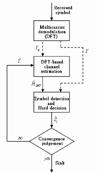
3.5 Flowchart of the iterative joint channel estimation and symbol detection (JCESD) algorithm. . . 44

4.1 Block diagram of the TMS320C6416 DSP [22]. . . 47

4.2 Pipeline phases of TMS320C6416 DSP [22]. . . 49

4.3 TMS320C64x CPU data paths [22]. . . 53

4.4 Block diagram of the Quixote board [21]. . . 55

4.5 Illustration of the DSP streaming mode [21]. . . 56

4.6 Code development flow for TI C6000 DSP [28]. . . 61

5.1 Block diagram of the simulated system (from [29]). . . 67

5.2 Channel estimation steps (from [29]). . . 67

5.3 The SER curve for uncoded QPSK resulting from simulation matches the theoretical one. . . 69

5.4 (a) Amplitude response and (b) phase response of the multipath channel at a certain time instant. . . 70

5.5 (a) MSE and (b) SER for QPSK in multipath channel estimation without utilization of the preamble. . . 72

5.6 Fixed-point data formats in our design. . . 73

5.7 (a)MSE and (b)SER for different interpolation order. . . 76

(18)

5.9 Performance at worst and best subcarriers. (a) MSE. (b) SER. . . 78

5.10 Program structure for channel estimation. . . 78

5.11 Function Modulation (QPSK). . . . 79

5.12 Function Complex Mul. . . . 79

5.13 Function Linear Interp. . . . 80

5.14 Function SecondOrder Interp. . . . 81

5.15 Function Complex Div. . . . 82

5.16 Function De-modulation(QPSK). . . . 82

5.17 Assembly code of function Modulation (QPSK). . . . 83

5.18 Assembly code of function Complex Mul. . . . 84

5.19 Assembly code of function Linear Interp. . . . 85

5.20 Assembly code of function SecondOrder Interp. . . . 86

5.21 Assembly code of function Complex Div. . . . 87

5.22 Assembly code of function De-modulation(QPSK). . . . 88

5.23 Software pipelining information of 16-bit fixed-point Complex Mul. . . . 89

6.1 Amplitude variations for different velocities. (a) v = 60 km/h. (b) v = 120 km/h. (c) v = 180 km/h. (d) v = 240 km/h. (e) v = 300 km/h. (f) v = 360 km/h. . . 93

6.2 Resampling a nonsample-spaced channel extends the channel (from [3]). . . . 94

6.3 Simulation results (1D linear interpolation) for AWGN channel. (a) MSE. (b) SER. . . 95

(19)

6.4 The path extension effect in our model. (a) Nonsample-spaced multipath

channel. (b) Equivalent sample-spaced multipath channel. . . 96

6.5 OFDMA DL PUSC MSE and SER for v = 60 km/h in each modulation scheme. (a) MSE for QPSK. (b) SER for QPSK. (c) MSE for 16QAM. (d) SER for 16QAM. (e) MSE for 64QAM. (f) SER for 64QAM. . . 97

6.6 MSE and SER spread over used subcarriers in QPSK at 30 dB. . . 98

6.8 The performance of 1D linear interpolation for different velocity with 16QAM. (a) MSE. (b) SER. . . 99

6.9 Performance of 2D interpolation for v = 60 km/h with 16QAM. (a) MSE. (b) SER. . . 100

6.10 Performance of 2D-(21) interpolation for different velocities with 16QAM. (a) MSE. (b) SER. . . 100

6.11 Performance of linear prediction using different merit functions. (a) MSE. (b) SER. . . 101

6.12 Performance of time-averaging. (a) SER for averaging 4 symbols (b) SER for averaging 6 symbols . . . 102

6.13 OFDMA DL FUSC MSE and SER for v = 60 km/h in each modulation scheme. (a) MSE for QPSK. (b) SER for QPSK. (c) MSE for 16QAM. (d) SER for 16QAM. (e) MSE for 64QAM. (f) SER for 64QAM. . . 104

6.14 MSE and SER spread over used subcarriers in QPSK at 30 dB. . . 105

(20)

6.17 NLMS performance based on equalization. (a) MSE for QPSK. (b) SER for QPSK. . . 107 6.18 NLMS performance based on channel estimation. (a) MSE for QPSK. (b)

SER for QPSK. . . 107 6.19 Maximum likelihood channel estimators for different computational precision.

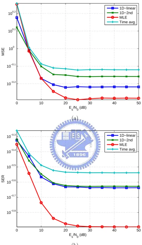
(a) MSE. (b) SER. . . 109 6.20 Eigenvalue spread of the matrix D in (3.27). . . 110 6.21 Maximum likelihood versus joint channel estimation and symbol detection.

(a) MSE. (b) SER. . . 111 6.22 Performance of JCESD with different number of iterations. (a) MSE. (b) SER.111 6.23 PUSC mode versus FUSC mode (1D-2nd interpolation). (a) MSE. (b) SER. 113 6.24 Comparison of channel estimation techniques. (a) MSE. (b) SER. . . 114

(21)

List of Tables

2.1 OFDM Symbol Parameters (from [4]) . . . 14

2.2 OFDMA DL Subcarrier Allocation under PUSC [4], [5] . . . 21

2.3 OFDMA DL Subcarrier Allocation under FUSC [4], [5] . . . 24

4.1 Execution Stage Length Description for Each Instruction Type [22] . . . 50

4.2 Functional Units and Operations Performed [22] . . . 51

5.1 OFDM Uplink Parameters . . . 66

5.2 Power-Delay Profile of the ETSI “Vehicular A” Channel . . . 66

5.3 Q1.14 Bit Fields . . . 73

5.4 Profile of the Channel Estimator Implementation . . . 74

(22)

Chapter 1 Introduction

Oncoming technologies such as WiFi and WiMAX are changing wireless communication. The demand for high data rate transmission and multimedia type traffic grows rapidly. Due to its inherent advantages in high-speed communication, orthogonal frequency division multiplexing (OFDM) has become the choice for a number of high wireless systems (e.g., DVB-T, WiFi, WiMAX).

OFDM system transmits data using a set of parallel low bandwidth subcarriers. The subcarriers are independent from each other even though their spectra overlap, which results in its bandwidth efficiency and resistance to the ICI (inter-carrier interference) effect. And due to the low bandwidth of subcarriers, each subcarrier can avoid worse subchannels. Thus ISI (inter-symbol-interference) is also reduced. High data rate systems are also achieved by using a large number of carriers. OFDM can be easily generated using an inverse fast Fourier transform (IFFT) and received using a fast Fourier transform (FFT).

The IEEE 802.16 standard committee has developed a group of standards for wireless metropolitan area networks (MANs). The original 802.16 standard specifies the air interface for fixed broadband wireless access systems supporting multimedia services. The medium access control layer (MAC) supports a primarily point-to-multipoint architecture, with an

(23)

optional mesh topology. The MAC is structured to support multiple physical layer (PHY) specifications, each suited to a particular operational environment. For operational frequen-cies from 10–66 GHz, the WirelessMAN-SC PHY, based on single-carrier modulation, is specified. For frequencies below 11 GHz, where propagation without a direct line of sight must be accommodated, three alternatives are provided in the later 802.16a: WirelessMAN-OFDM (using orthogonal frequency-division multiplexing), WirelessMAN-WirelessMAN-OFDMA (using orthogonal frequency-division multiple access), and WirelessMAN-SCa (using single-carrier modulation).

IEEE 802.16 has developed the IEEE Standard 802.16-2004 for broadband wireless access systems, which provides a variety of services to fixed outdoor as well as nomadic indoor users. Work is underway on a mobile extension, referred to as Project 802.16e, supporting new capabilities needed for the mobile environment. The object of this thesis focus on the channel estimation part for WirelessMAN-OFDM and WirelessMAN-OFDMA.

This thesis is organized as follows. First, in chapter 2, we introduce some OFDM basics together with the IEEE 802.16e OFDM uplink and OFDMA downlink standard. In chapter 3, the various channel estimation techniques are introduced. In chapter 4, we describe the implementation platform, which consists of Texas Instrument’s TMS320C6416 digital signal processor (DSP) on a cPCI board named Quixote made by Innovative Integration. Then in chapter 5, we discuss the performance of channel estimation methods of OFDM uplink and some DSP implementation issues. The simulation results of OFDMA downlink will be left to chapter 6. At last, we give the conclusion and discuss potential future work in chapter 7.

(24)

Chapter 2 Introduction to IEEE802.16e OFDM

and OFDMA

This chapter presents a brief overview of the OFDM and the OFDMA techniques for mul-ticarrier modulation. The OFDM uplink and OFDMA downlink specifications of IEEE 802.16e are also introduced.

2.1 Basics of OFDM and OFDMA

The basic idea of OFDM-like or OFDMA-like system is to split the data stream into several parallel streams, each transmitted on a separate subcarrier. Moreover, these subcarriers are made orthogonal is to allow spectral overlapping and better spectral efficiency can be achieved. Material in this section is taken from [1], [2] and [3].

Figure 2.1 shows the block diagram of a simplex transmission system using OFDM. The three main principles incorporated are as follows:

1. The IDFT and the DFT are used for modulating and demodulating the data constel-lations on the orthogonal subcarriers. These signal processing algorithms replace the banks of I/Q-modulators and demodulators that would otherwise be required. Usually,

(25)

N is taken as an integer power of two, enabling the application of the efficient FFT

algorithms for modulation and demodulation.

2. The second key principle is the introduction of a cyclic prefix, whose length should ex-ceed the maximum excess delay of the multipath propagation channel. Due to the cyclic prefix, the transmitted signal becomes periodic, and the effect of the time-dispersive multipath channel is equivalent to a cyclic convolution, after discarding the cyclic pre-fix at the receiver. Owing to the properties of the cyclic convolution, the effect of the multipath channel is limited to a pointwise multiplication of the data constellations by the channel transfer function. The only drawback of this principle is a slight loss of effective transmit power. The equalization (symbol demapping) required for detect-ing the data constellations (when there is no error control coddetect-ing) is an elementwise multiplication of the DFT output by the inverse of the estimated channel transfer function.

3. FEC (forward error control) coding and interleaving are usually also applied. The frequency-selective radio channel may severely attenuate the data symbols transmitted on one or several subcarriers. Spreading the coded bits over the bandwidth, an efficient coding scheme can correct the erroneous bits and hence exploit the frequency diversity. Synchronization is a key issue in the design of a robust OFDM receiver. Time and frequency synchronization are paramount to identify the start of the OFDM symbol and to align local oscillator frequencies.

2.1.1 The OFDM Principle

For multicarrier modulation, the available bandwidth W is divided into a number Nc of

(26)

Figure 2.1: OFDM system block diagram (from [2]).

bandwidth is illustrated in Fig. 2.2, where arrows represent the different subcarriers. Instead of transmitting the data symbols in a serial way, at a baud rate R, a multicarrier transmitter partitions the data stream into blocks of Ncdata symbols that are transmitted in parallel by

modulating the Nc carriers. The symbol duration for a multicarrier scheme is Ts= Nc/R.

As shown in Fig. 2.3, the general form of the multicarrier signal can be written as a set of modulated carriers: s(t) = ∞ X m=−∞ ¡NXc−1 k=0 xk,mψk(t − mTs) ¢ (2.1) where xk,m is the data symbol modulating the kth subcarrier in the mth signalling interval

and ψk is the waveform for the kth subcarrier.

The symbol duration can be made long compared to the maximum excess delay of the channel, Ts À τmax, or by choosing Nc sufficiently high. At the same time, the

band-width of the subbands can be made small to reduce the coherence bandband-width of the channel

(Bcoh À W/Nc). The subbands then experience flat fading, which reduces equalization to a

signal complex multiplication per carrier. Hence, increasing Nc reduces the ISI (intersymbol

interference) effects.

(27)

Figure 2.2: Subdivision of the bandwidth into Nc subbands (from [3]).

Figure 2.3: Multicarrier modulation (from [3]).

coherence time Tcoh of the channel is small compared to Ts, the channel frequency response

changes significantly during the transmission of one symbol. As a result, the coherence time of the channel defines an upper bound for the number of subcarriers. Together with the condition for flat fading within the subbands, a reasonable range for Nc is given by

W

Bcoh

¿ Nc¿ RTcoh. (2.2)

(28)

Figure 2.4: Spectrum of an OFDM signal (from [3]).

spectra. A general set of orthogonal waveforms is given by:

ψk(t) = ½ ₁ √ Tse jωkt, t ∈ [0, T s], 0, otherwise, (2.3) where ωk= ω0+ kωs and k = 0, 1, . . . , Nc− 1. Here fk = ωk/2π is the subcarrier frequency

and f0 = w0/2π is the lowest frequency used (k = 0). The spacing between the adjacent subcarriers equals ∆f = ωs/2π = W/Nc. Since the waveform ψk(t) is restricted to the time

window [0, Ts], the intercarrier spacing must also satisfy 4f = 1/Ts= R/Nc. The windowing

results in a convolution with Ts· exp(−jπf Ts) · sin(πf T_{πf T}_ss) in the frequency domain. How the

subbands overlap is shown in Fig. 2.4.

2.1.2 Cyclic Prefix

As mentioned, to overcome the ISI and ICI (interchannel interference) problem, the cyclic prefix (CP) is introduced. A cyclic prefix is a copy of the last part of the OFDM symbol (see Fig. 2.5). The cyclic prefix should be at least as long as the significant part of the channel impulse response. The benefit of the CP is twofold. First, it avoids ISI because it acts as a guard space between successive symbols. Second, it also converts the linear convolution with channel impulse response into a cyclic convolution. However, the transmitted energy

(29)

Figure 2.5: Cyclic prefix (form [3]).

increases with the length of the CP. The SNR loss is given by

SNRloss= −10 log10(1 −

Tg

Ts

). (2.4)

2.1.3 Discrete-Time Equivalent System Model

The discete-time baseband equivalent model is shown in Fig. 2.6. In the transmitter, the data stream is grouped in blocks of Ncdata symbols. These groups are called OFDM symbols and

can be represented by a vector xm = [x0,m x1,m · · · xNc−1,m]T. Then an IDFT is performed

on each data symbol block, and a cyclic prefix of length Ncpis added. The resulting complex

baseband discrete time signal of mth OFDM-symbol can be written as

sm(n) =    1 Nc NPc−1 k=0 xk,mej2πk(n−Ncp)/Nc, if n ∈ [0, Nc+ Ncp− 1], 0, otherwise. (2.5)

The complete time signal s(n) is given by the concatenation of all OFDM symbols that are transmitted: s(n) = ∞ X m=0 sm(n − m(Nc+ Ncp)). (2.6)

Here we assume that

• The channel fading is slow enough to consider it constant during one OFDM symbol. • The transmitter and receiver are perfectly synchronized.

(30)

Figure 2.6: Discrete-time baseband equivalent model (from [3]).

• The CP is sufficiently long to accommodate the channel impulse response.

We can then write

r(n) =

N_Xcp−1

η=0

h(η)s(n − η) + n(n). (2.7)

In the receiver, the incoming sequence is split into blocks and the cyclic prefix associated with each clock is removed. This results in a vector rm= [r(zm) r(zm+1) · · · r(zm+Nc−1)]T,

with zm = m(Nc+ Ncp) + Ncp. Performing DFT on rm yields

yk,m=

NXc−1

n=0

r(zm+ n)e−j2πkn/Nc. (2.8)

Substituting r(n) in (2.7) into (2.8) gives

yk,m= NXc−1 n=0 ·N_Xcp−1 η=0 h(η)sm(Ncp + n − η) ¸ e−j2πkn/Nc ₊ NXc−1 n=0 n(zm+ n)e−j2πkn/Nc. (2.9)

Then substituting sm(n) in (2.5) into it yields

yk,m= NXc−1 n=0 ·N_Xcp−1 η=0 h(η) 1 Nc NXc−1 k=0 xk,mej2πk(n−η)/Nc ¸ e−j2πkn/Nc _{+ n} k,m (2.10) where nk,m= NPc−1 n=0

n(zm+ n)e−j2πkn/Nc is the kth sample of the Nc-point DFT of n(zm+ n).

(31)

Note that h(η) = 0 for all η > Ncp − 1. Additional swapping the two inner sums and reordering yields yk,m= NXc−1 n=0 h 1 Nc NXc−1 k=0 ¡NXc−1 η=0 h(η)e−j2πkη/Nc¢_x k,mej2πkn/Nc | {z } IDF T i e−j2πkn/Nc | {z } DF T +nk,m. (2.11)

The first part of this expression consists of an IDFT operation nested in a DFT operation. The inner sum is the kth sample of the Nc-point DFT of h(n), or hk. The equation hence

translates into

yk,m = hkxk,m+ nk,m. (2.12)

This equation demonstrates that the received data symbol yk,m on each subcarrier k

equals the data symbol xk,m, multiplied by the corresponding frequency-domain channel

coefficient hk in addition to the transformed noise nk,m.

For a more compact notation, a matrix equivalent is often used. For a single OFDM symbol, it equals

ym = H ◦ xm+ nm = diag(H) · xm+ nm (2.13) where ◦ denotes the element-wise product, diag(H) is the diagonal matrix of the elements of

H, ym = [y0,my1,m · · · yNc−1,m]T, nm = [n0,mn1,m · · · nNc−1,m]T and H = [h0h1 · · · hNc−1]T.

2.2 Generic OFDM and OFDMA Symbol Description

for IEEE 802.16e

2.2.1 Time Domain Description

IDFT creates the OFDM symbol waveforms. The time duration of each OFDM symbol is referred to as the useful symbol time Ts. A copy of the last Tcp of the useful symbol period

(32)

Figure 2.7: OFDM frequency description (from [4]).

by increasing the FFT size, which would however, among other things, adversely affect the sensitivity of the system to phase noise of the oscillators. Using a cyclic extension, the samples required for performing the FFT at the receiver can be taken anywhere over the length of the extended symbol. This provides multipath immunity as well as a tolerance for symbol time synchronization errors.

2.2.2 Frequency Domain Description

An OFDM (see Fig. 2.7) or OFDMA (see Fig. 2.8) symbol is made up from several carrier types:

• Data carriers: For data transmission.

• Pilot carriers: For various estimation purposes.

• Null carriers: No transmission ar all, for guard bands, non-active subcarriers and the

DC subcarrier.

2.2.3 Primitive Parameters

Four primitive parameters characterize the OFDM and the OFDMA symbols:

(33)

Figure 2.8: OFDMA frequency description (from [4]).

• Nused: Number of used subcarriers.

• n: Sampling factor. This parameter, in conjunction with BW and Nused, determines

the subcarrier spacing and the useful symbol time.

• G: This is the ratio of CP time to “useful” time, i.e., Tcp/Ts.

2.2.4 Derived Parameters

The following parameters are defined in terms of the primitive parameters.

• NF F T: Smallest power of two greater than Nused.

• Sampling frequency: Fs = f loor(n·BW/8000) × 8000.

• Subcarrier spacing: 4f = Fs/NF F T.

• Useful symbol time: Ts= 1/4f .

• CP time: Tcp = G × Ts.

• OFDM or OFDMA symbol time: T = Ts+ Tcp.

(34)

Figure 2.9: PEV EN time domain structure (from [4]).

2.3 OFDM Uplink Specifications in IEEE 802.16e

This section introduces the IEEE 802.16e OFDM uplink (UL) standard. The material is mainly taken from [4] and [5]. The parameters are given in Table 2.1. Note that Table 2.1 also indicates the pilot locations and the subchannelization method which will not be detailed later.

2.3.1 OFDM UL Preamble Structure and Modulation

In the uplink, the data preamble is as shown in Fig. 2.9. It consists of one OFDM symbol utilizing only even subcarriers. The time domain waveform consists of 2 times 128 samples preceded by a CP. The subcarrier values shall be set as

PEV EN(k) =

½ √

2 · PALL(k), k mod 2 = 0,

(35)

(36)

where PALL(−100 : 100) = {1 − j, 1 − j, −1 − j, 1 + j, 1 − j, 1 − j, −1 + j, 1 − j, 1 − j, 1 − j, 1 + j, −1 − j, 1 + j, 1 + j, −1 − j, 1 + j, −1 − j, −1 − j, 1 − j, −1 + j, 1 − j, 1 − j, −1 − j, 1 + j, 1 − j, 1 − j, −1 + j, 1 − j, 1 − j, 1 − j, 1 + j, −1 − j, 1 + j, 1 + j, −1 − j, 1 + j, −1 − j, −1 − j, 1 − j, −1 + j, 1 − j, 1 − j, −1 − j, 1 + j, 1 − j, 1 − j, −1 + j, 1 − j, 1 − j, 1 − j, 1 + j, −1 − j, 1 + j, 1 + j, −1 − j, 1 + j, −1 − j, − 1 − j, 1 − j, −1 + j, 1 + j, 1 + j, 1 − j, −1 + j, 1 + j, 1 + j, −1 − j, 1 + j, 1 + j, 1 + j, −1 + j, 1 − j, −1 + j, −1 + j, 1 − j, −1 + j, 1 − j, 1 − j, 1 + j, −1 − j, −1 − j, − 1 − j, −1 + j, 1 − j, −1 − j, −1 − j, 1 + j, −1 − j, −1 − j, −1 − j, 1 − j, −1 + j, 1 − j, 1 − j, −1 + j, 1 − j, −1 + j, −1 + j, −1 − j, 1 + j, 0, −1 − j, 1 + j, −1 + j, − 1 + j, −1 − j, 1 + j, 1 + j, 1 + j, −1 − j, 1 + j, 1 − j, 1 − j, 1 − j, −1 + j, −1 + j, − 1 + j, −1 + j, 1 − j, −1 − j, −1 − j, −1 + j, 1 − j, 1 + j, 1 + j, −1 + j, 1 − j, 1 − j, 1 − j, −1 + j, 1 − j, −1 − j, −1 − j, −1 − j, 1 + j, 1 + j, 1 + j, 1 + j, −1 − j, −1 + j, − 1 + j, 1 + j, −1 − j, 1 − j, 1 − j, 1 + j, −1 − j, −1 − j, −1 − j, 1 + j, −1 − j, −1 + j, − 1 + j, −1 + j, 1 − j, 1 − j, 1 − j, 1 − j, −1 + j, 1 + j, 1 + j, −1 − j, 1 + j, −1 + j, − 1 + j, −1 − j, 1 + j, 1 + j, 1 + j, −1 − j, 1 + j, 1 − j, 1 − j, 1 − j, −1 + j, −1 + j, − 1 + j, −1 + j, 1 − j, −1 − j, −1 − j, 1 − j, −1 + j, −1 − j, −1 − j, 1 − j, −1 + j, − 1 + j, −1 + j, 1 − j, −1 + j, 1 + j, 1 + j, 1 + j, −1 − j, −1 − j, −1 − j, −1 − j, 1 + j, 1 − j, 1 − j}.

2.3.2 OFDM UL Pilot Modulation

Pilot subcarriers shall be inserted into each data burst in order to constitute the symbol. The PRBS (pseudo-random binary sequence) generator depicted in Fig. 2.10 shall be used

(37)

Figure 2.10: PRBS for pilot modulation (from [4]).

to produce a sequence, wk. The polynomial for the PRBS generator is X11+ X9+ 1.

The initialization sequence shown in Fig. 2.10 shall be used on the downlink (DL) and uplink. The value of the pilot modulation for OFDM symbol k is derived from wk. On both

uplink and downlink, the first symbol of the preamble is denoted by k = 0. For each pilot, the BPSK modulation shall be as follows:

DL : c−88= c−38 = c63= c88= 1 − 2wk and c−63= c−13 = c13= c38 = 1 − 2wk, (2.15)

UL : c−88= c−38 = c13= c38 = c63= c88= 1 − 2wk and c−63= c−13 = 1 − 2wk. (2.16)

2.3.3 OFDM UL Data Modulation

The OFDM data modulation schemes are shown in Fig. 2.11. The data bits are entered serially to the constellation mapper. BPSK, Gray-mapped QPSK, Gray-mapped 16QAM and Gray-mapped 64QAM must be supported. The indicated factor c is used to achieve equal average power.

The constellation-mapped data shall be subsequently modulated onto all allocated data subcarriers in order of increasing frequency offset index. The first symbol out of the data

(38)

Figure 2.11: BPSK, QPSK, 16QAM and 64QAM constellations (from [4]).

constellation mapping shall be modulated onto the allocated subcarrier with the lowest frequency offset index.

2.4 OFDMA Downlink Specifications in IEEE 802.16e

This section briefs the IEEE 802.16e OFDMA downlink standard. Both the PUSC (Partial Usage of SubChannels) and FUSC (Full Usage of SubChannels) are introduced. The material is mainly taken from [4] and [5].

2.4.1 Definition of OFDMA Basic Terms

In OFDMA, a slot in the OFDMA PHY is a two-dimensional entity spanning both a time and a subchannel dimension. It is the minimum possible data allocation unit.

(39)

• For downlink FUSC, one slot is one subchannel by one OFDMA symbol. • For downlink PUSC, one slot is one subchannel by two OFDMA symbols.

A Data Region is a two-dimensional allocation of a group of contiguous subchannels, in a group of contiguous OFDMA symbols; a segment is a subdivision of the set of available OFDMA subchannels.

The downlink data mapping rules are as follows:

1. Segment the data after the modulation block into blocks sized to fit into one OFDMA slot.

2. Each slot shall span one subchannel in the subchannel axis and one or more OFDMA symbols in the time axis, as per the slot definition mentioned before. Map the slots such that the lowest numbered slot occupies the lowest numbered subchannel in the lowest numbered OFDMA symbol.

3. Continue the mapping such that the OFDMA subchannel index is increased. When the edge of the Data Region is reached, continue the mapping from the lowest numbered OFDMA subchannel in the next available symbol.

Figure 2.12 illustrates the order in which OFDMA slots are mapped to subchannels and OFDMA symbols.

2.4.2 OFDMA DL Preamble Structure and Modulation

The first symbol of the downlink transmission is the preamble. There are three types of preamble carrier-sets, which are defined by allocation of different subcarriers for each one of them. The subcarriers are modulated using a boosted BPSK modulation with a specific PN

(40)

Figure 2.12: Example of mapping OFDMA slots to subchannels and symbols in the downlink in PUSC mode (from [5]).

(pseudo-noise) code. The PN series modulating the preamble carrier-sets can be found in [4, pp. 553–562]. The preamble carrier-sets are defined as

P reambleCarrierSetn= n + 3 · k, (2.17)

where:

• P reambleCarrierSetn specifies all subcarriers allocated to the specific preamble,

• n is the number of the preamble carrier-set indexed 0, 1, 2, • k is a running index 0,. . . ,567.

Each segment uses one type of preamble out of the three sets in the following manner: The DC carrier will not be modulated at all and the appropriate PN will be discarded. Therefore, DC carrier shall always be zeroed. For the preamble symbol, there will be 172 guard band

(41)

Figure 2.13: Cluster structure (from [5]).

subcarriers on both the left side and on the right side of the spectrum. Segment i uses preamble carrier-set i, where i = 0, 1, 2.

The pilot in downlink preamble shall be modulated as

<{P reambleP ilotsModulated} = 4 ·√2 ·¡1 2 − wk ¢ , ={P reambleP ilotsModulated} = 0. (2.18)

2.4.3 OFDMA DL Carrier Allocation

For both uplink and downlink in OFDMA, Nusedsubcarriers are allocated to pilot subcarriers

and data subcarriers. In the downlink, the pilot tones are allocated first; what remains are data subcarriers, which are divided into subchannels that are used exclusively for data. Table 2.2 summarizes the parameters of the OFDMA PUSC symbol structure and Table 2.3 the corresponding parameters of OFDMA FUSC.

2.4.3.1 PUSC DL

The OFDMA symbol structure is constructed using pilots, data and zero subcarriers. The symbol is first divided into basic clusters and zero carriers are allocated. Pilots and data carriers are allocated within each cluster. Figure 2.13 shows the cluster structure with subcarriers from left to right in order of increasing subcarrier index.

(42)

Table 2.2: OFDMA DL Subcarrier Allocation under PUSC [4], [5] Parameter Value Comments

Number of DC subcarriers

1 Index 1024 (counting from 0) Number of guard subcarriers, left 184 Number of guard subcarriers, right 183 Number of used subcarriers (Nused)

1681 Number of all subcarriers used within a symbol, including all possible allocated pilots and the DC carrier

Number of subcarriers per cluster

14 Number of clusters 120

Renumbering sequence 1 Used to renumber clusters before allocation to subchannels: 6,108,37,81,31,100,42,116,32,107,30,93,54,78, 10,75,50,111,58,106,23,105,16,117,39,95,7, 115,25,119,53,71,22,98,28,79,17,63,27,72,29, 86,5,101,49,104,9,68,1,73,36,74,43,62,20,84, 52,64,34,60,66,48,97,21,91,40,102,56,92,47, 90,33,114,18,70,15,110,51,118,46,83,45,76,57, 99,35,67,55,85,59,113,11,82,38,88,19,77,3,87, 12,89,26,65,41,109,44,69,8,61,13,96,14,103,2, 80,24,112,4,94,0 Number of data subcarriers in each symbol per subchannel

24 Number of subchannels 60 Basic permutation sequence 12 (for 12 subchannels) 12 6,9,4,8,10,11,5,2,7,3,1,0 Basic permutation sequence 8 (for 8 subchannels) 8 7,4,0,2,1,5,3,6

1) Dividing the subcarriers into the number (Nclusters) of physical clusters containing 14

(43)

2) Renumbering the physical clusters into logical clusters using the following formula: LogicalCluster =   

RenumberingSequence(P hysicalCluster), first DL zone,

RenumberingSequence¡(P hysicalCluster+

13 · DL P ermBase)mod Nclusters

¢

, otherwise.

3) Dividing the clusters into six major groups. Group 0 includes clusters 0–23, group 1 clusters 24–39, group 2 clusters 40–63, group 3 clusters 64–79, group 4 clusters 80– 103 and group 5 clusters 104–119. These groups may be allocated to segments. If a segment is being used, then at least one group shall be allocated to it. (By default group 0 is allocated to sector 0, group 2 to sector 1, and group 4 to sector 2).

4) Allocating subcarriers to subchannels in each major group as

subcarrier(k, s) = Nsubchannels· nk+

©

ps[nk mod Nsubchannels]+

DL P ermBaseªmod Nsubchannels.

where:

• subcarrier(k, s) is the subcarrier index of subcarrier k in subchannel s; • nk= (k + 13 · s)mod Nsubcarriers;

• Nsubchannels is the number of subchannels (for PUSC use number of subchannels

in the currently partitioned group);

• ps[j] is the series obtained by rotating basic permutation sequence cyclically to

the left s times;

• Nsubcarriers is the number of data subcarriers allocated to a subchannel in each

OFDMA symbol;

(44)

2.4.3.2 FUSC DL

In comparison with PUSC, the subcarrier allocation and subchannelization methods for FUSC are much simpler. For data subcarrier allocation and subchannelization, use the parameters listed in Table 2.3 and apply the same carrier allocation procedures mentioned in PUSC part. As for pilot allocation, use

P ilotsLocation =£V ariableSet#x + 6 · (F USC SymbolNumber mod 2)¤

∪ConstantSet#0 ∪ ConstantSet#1.

2.4.4 OFDMA DL Pilot Modulation

In OFDMA, the polynomial for PRBS generator is X11_{+ X}9_{+ 1, which is the same as that} in OFDM system. However, in this case, the initialization vector used to generate wk shall

refer to the MAC layer and is not introduced here. The interested reader can get detailed information from [5, pp. 631–632].

In both FUSC and PUSC modes, each pilot shall be transmitted with a boosting of 2.5 dB over the average non-boosted power of each data tone. The pilot subcarriers shall be modulated according to as <{ck} = 8 3 ¡1 2 − wk ¢ , ={ck} = 0. (2.19)

2.4.5 OFDMA DL Data Modulation

As shown in Fig. 2.11, in the OFDMA system, the data bits are entered serially to the constellation mapper. Gray-mapped QPSK and Gray-mapped 16QAM shall be supported, whereas the support of 64QAM (also Gray-mapped) is optional and BPSK is not supported.

(45)

Table 2.3: OFDMA DL Subcarrier Allocation under FUSC [4], [5] Parameter Value Comments

Number if DC subcarriers

1 Index 1024 (counting from 0) Number of Guard subcarriers, Left 173 Number of Guard subcarriers, Right 172 Number of used subcarriers (Nused)

1703 Number of all subcarriers used within a symbol, including all possible allocated pilots and the DC carrier Pilots VariableSet #0 71 0,72,144,216,288,360,432,504,576,648,720,792,864, 936,1008,1080,1152,1224,1296,1368,1440,1512,1584, 1656,48,120,192,264,336,408,480,552,624,696,768, 840,912,984,1056,1128,1200,1272,1344,1416,1488, 1560,1632,24,96,168,240,312,384,456,528,600,672, 744,816,888,960,1032,1104,1176,1248,1320,1392, 1464,1536,1608,1680 ConstantSet #0 12 9,153,297,441,585,729,873,1017,1161,1305,1449, 1593 VariableSet #1 71 36,108,180,252,324,396,468,540,612,684,756,828, 900,972,1044,1116,1188,1260,1332,1404,1476,1548, 1620,1692,12,84,156,228,300,372,444,516,588,660, 732,804,876,948,1020,1092,1164,1236,1308,1380, 1452,1524,1596,1668,60,132,204,276,348,420,492, 564,636,708,780,852,924,996,1068,1140,1212,1284, 1356,1428,1500,1572,1644 ConstantSet #1 12 81,225,369,513,657,801,945,1089,1233,1377,1521, 1665 Number of data subcarriers 1536 Number of data subcarriers per subchannel 48 Number of sunchannels 32 Basic permutation sequence 32 3,18,2,8,16,10,11,15,26,22,6,9,27,20,25,1,29, 7,21,5,28,31,23,17,4,24,0,13,12,19,14,30

(46)

It is worth noting that before mapping the data to the physical subcarriers, each sub-carrier shall be multiplied by the factor 2 × (1/2 − wk) according to the subcarrier physical

(47)

Chapter 3 Channel Estimation Techniques

3.1 Pilot-Symbol-Aided Channel Estimation

Channel estimators usually need some kind of pilot information as a point of reference. A fading channel requires constant tracking, so pilot information has to be transmitted more or less continuously. Decision-directed channel estimation can also be used. But even in these types of schemes, pilot information has to be transmitted regularly to mitigate error propagation [6].

3.1.1 The Least-Squares (LS) Estimator

The simplest channel estimator one can imagine consists simply in dividing the received signal by the symbols that have been actually sent (and that are supposed to be known). Based on a priori known data, we can estimate the channel information on pilot carriers roughly by the least-squares (LS) estimator. An LS estimator minimizes the following squared error [7]:

||Y − ˆHLSX||2 (3.1)

where Y is the received signal and X is a priori known pilots, both in the frequency domain and both being N × 1 vectors where N is the FFT size. ˆHLS is an N × N matrix whose

(48)

values are 0 except at pilot locations mi where i = 0, · · · , Np − 1: ˆ HLS =       Hm0,m0 · · · 0 · · · 0 · · · 0 0 · · · Hm1,m1 · · · 0 · · · 0 0 · · · 0 · · · Hm2,m2 · · · 0 0 · · · 0 · · · 0 · · · 0 0 · · · 0 · · · 0 · · · HmNp−1,H_mNp−1      . (3.2)

Therefore, (3.1) can be rewritten as

[Y (m) − ˆHLS(m)X(m)]2, for all m = mi. (3.3)

Then the estimate of pilot signals, based on only one observed OFDM symbol, is given by ˆ HLS(m) = Y (m) X(m) = X(m)H(m) + N(m) X(m) = H(m) + N(m) X(m) (3.4)

where N(m) is the complex white Gaussian noise on subcarrier m. We collect HLS(m) into

ˆ

Hp,LS, an Np× 1 vector where Np is the total number of pilots, as

ˆ Hp,LS = [Hp,LS(0) Hp,LS(1) · · · Hp,LS(Np− 1)]T = [Yp(0) Xp(0), Yp(1) Xp(1), . . . , Yp(Np−1) Xp(Np−1)] T_. (3.5)

The LS estimate of Hp based on one OFDM symbol is susceptible to noise effects, and thus

an estimator better than the LS estimator is preferable.

3.1.2 The LMMSE Estimator

The minimum mean-square error (MMSE) estimate has been shown to be better than the LS estimate for channel estimation in OFDM systems, but the major drawback of the MMSE estimate is its high complexity. A low-rank approximation results in a linear minimum mean squared error (LMMSE) estimator that uses the frequency-domain correlation of the channel [8]. The linear minimum mean-square error channel estimator tries to minimize the mean squared error between the actual and estimated channels, obtained by a linear transformation

(49)

applied to ˆHp,LS. The mathematical representation of the LMMSE estimator on pilot signals is ˆ Hp,lmmse = RHpHp,LSR −1 Hp,LSHp,LSHˆp,LS = RHpHp(RHpHp+ σ 2 n(XpXHp )−1)−1Hˆp,LS (3.6)

where ˆHp,LS is the least-square estimate of Hp in (3.5), σn2 is the variance of the Gaussian

white noise, Xp is the vector of transmitted signal on pilot subcarriers, and the covariance matrices are defined by

RHpHp,LS = E{HpH H p,LS}, (3.7) RHp,LSHp,LS = E{Hp,LSH H p,LS}, (3.8) RHpHp = E{HpH H p }. (3.9)

Note that there is a matrix inverse involved in the MMSE estimator, which must be calculated every time, and the computation of matrix inversion requires O(N3

p) arithmetic operations

[9]. We also need the statistical properties of the unknown channel. Therefore, we use the LS estimator which requires only O(Np) operations instead of the LMMSE due to the concerns

of complexity and unknown information.

3.2 One-Dimensional Channel Estimators

By one-dimensional channel estimation, we mean that we only use channel information along the frequency domain. In other words, we use the channel information at pilot subcarriers obtained by the LS estimator to estimate the channel information at data subcarriers via interpolation or extrapolation. The material in this section is largely taken from [10].

(50)

3.2.1 Polynomial Interpolation and Extrapolation

The interpolation polynomial of degree N − 1 through the N points y1 = f (x1), y2 =

f (x2), . . . , yN = f (xN) is given by Lagrange’s classical formula as

P x = (x − x2)(x − x3) . . . (x − xN) (x1− x2)(x1− x3) . . . (x1− xN) y1+ (x − x1)(x − x3)(x − xN) (x2− x1)(x2− x3)(x2− xN) y2 + · · · + (x − x1)(x − x2)(x − xN −1) (xN − x1)(xN − x2)(xN − xN −1) yN. (3.10)

There are N terms, each a polynomial of degree N − 1 and each constructed to be zero at all of the xi except one, at which it is constructed to be yi.

A better method for constructing the interpolating polynomial is Neville’s algorithm as follows: Let P1 be the value at x of the unique polynomial of degree zero passing through the point (x1, y1); so P1 = y1. Likewise define P2, P3, . . . , PN. Now let P12 be the value at x of the unique polynomial of degree one passing through both (x1, y1) and (x2, y2). Likewise

P23, P34, . . . , P(N −1)N. Similarly, for higher-order polynomials, compute up to P123...N, which

is the value of the unique interpolating polynomial through all N points, i.e., the desired answer. The various P s form a “tableau” on the left lading to a single “descendent” at the extreme right. For example, with N = 4,

x1 : x2 : x3 : x4 : y1 = P1 y2 = P2 y3 = P3 y4 = P4 P12 P23 P34 P123 P234 P1234 (3.11)

Neville’s algorithm is a recursive way of filling in the numbers in the tableau a column at a time, from left to right. It is based on the relationship between a “daughter” P and its two “parents” as

Pi(i+1)...(i+m)=

(x − xi+m)Pi(i+1)...(i+m−1)+ (xi− x)P(i+1)(i+2)...(i+m)

(51)

This recurrence works because the two parents already agree at points xi+1, . . . , xi+m−1.

An improvement on the recurrence (3.12) is to keep track of the small differences between parents and daughters, namely, to define (for m = 1, 2, . . . , N − 1),

Cm,i ≡ Pi...(i+m)− Pi...(i+m−1),

Dm,i ≡ Pi...(i+m)− P(i+1)...(i+m).

(3.13) Then one can easily derive from (3.12) the relations

Dm+1,i =

(xi+m+1− x)(Cm,i+1− Dm,i)

xi− xi+m+1 , Cm+1,i = (xi− x)(Cm,i+1− Dm,i) xi− xi+m+1 . (3.14)

At each level m, the Cs and Ds are the corrections that make the interpolation one order higher. The final answer P1...N is equal to the sum of any yi plus a set of Cs and/or Ds that

form a path through the family tree to the rightmost daughter.

Usually, linear and second-order interpolations are employed due to the consideration of complexity, as discussed in [11], [12] and [13]. The mathematical expression of linear and second order interpolations are given below.

3.2.1.1 Linear interpolation The linear interpolation is given by

He(k) = He(m + l) = (Hp(m + 1) − Hp(m))

l

L + Hp(m) (3.15)

where Hp(k), k = 0, 1, · · · , Np, are the channel frequency responses at pilot subcarriers, L is

(52)

3.2.1.2 Second order interpolation The second-order interpolation is given by

He(k) = He(m + l) = c1Hp(m − 1) + c0Hp(m) + c−1Hp(m + 1) (3.16) where c1 = α(α − 1) 2 , c0 = −(α − 1)(α + 1), c−1 = α(α + 1) 2 , α = l L.

Other notations are the same as in linear interpolation.

3.2.2 Rational Function Interpolation and Extrapolation

Some functions are not well approximated by polynomials, but are well approximated by rational functions. We denote by Ri(i+1)...(i+m) a rational function passing through the m + 1

points (xi, yi), . . . , (xi+m, yi+m). Suppose

Ri(i+1)...(i+m)= Pµ(x) Qν(x) = p0+ p1x + · · · + pµx µ q0+ q1x + · · · + qνxν . (3.17) Since there are µ + ν + 1 unknown µs and νs (q0 being arbitrary), we must have m + 1 =

µ + ν + 1.

Rational functions are sometimes superior to polynomials because of their ability to model functions with poles, that is, zeros of the denominator of (3.17). These poles might occur for real values of x, if the function to be interpolated itself has poles. More often, the function

f (x) is finite for all finite real x, but has an analytic continuation with poles in the complex x-plane. Such poles can ruin a polynomial approximation, especially those at real values of x.

(53)

Bulirsch and Stoer found an algorithm of the Neville type which performs rational function extrapolation on tabulated data. The algorithm is summarized by a recurrence relation:

Ri(i+1)...(i+m) = R(i+1)...(i+m)+ R(i+1)...(i+m)− Ri...(i+m−1) ¡ _x−x i x−xi+m ¢¡ 1 − R(i+1)...(i+m)−Ri...(i+m−1) R(i+1)...(i+m)−R(i+1)...(i+m−1) ¢ − 1. (3.18)

This recurrence generates the rational functions through m + 1 points from the ones through

m and (the term R(i+1)...(i+m−1)) m − 1 points. It is started with

Ri = yi and R ≡ [Ri(i+1)...(i+m) with m = −1] = 0.

Now, we can convert the recurrence (3.18) to one involving only the small differences

Cm,i ≡ Ri...(i+m)− Ri...(i+m−1),

Dm,i ≡ Ri...(i+m)− R(i+1)...(i+m).

(3.19) Note that these satisfy the relation

Cm+1,i − Dm+1,i = Cm,i+1− Dm,i (3.20)

which is useful in proving the recurrences

Dm+1,i = ¡Cm,i+1_x−x_i(Cm,i+1− Dm,i)

x−xi+m+1 ¢ Dm,i− Cm,i+1 , Cm+1,i = ¡ _x−x i x−xi+m+1 ¢

Dm,i(Cm,i+1− Dm,i)

¡ _x−x i x−xi+m+1 ¢ Dm,i− Cm,i+1 . (3.21)

3.2.3 Cubic Spline Interpolation [10], [14], [15]

Cubic spline is one very effective, well-behaved, computationally efficient interpolation. The approach is to fit cubic polynomials to adjacent pairs of points and choose the values of the two remaining parameters associated with each polynomial such that the polynomials covering adjacent intervals agree with one another in both slope and curvature at their common endpoint. The cubic spline interpolation is developed in the following.

(54)

Given a tabulated function yi = y(xi) and its second order derivative y00, i = 1, . . . , N,

let us focus our attention on one particular interval, say between xj and xj+1. The goal of

cubic spline interpolation is to get an interpolation formula that is smooth in the first deriv-ative and continuous in the second derivderiv-ative, both within the interval and at its boundaries. A little calculation shows that there is only one way to arrange this construction, that is,

y = Ayi+ Byi+1+ cyj00+ Dy00j+1 (3.22)

where A, B, C and D are given by

A = xj+1− x xj+1− xj , B = 1 − A = x − xj xj+1− xj , C = 1 6(A 3_{− A)(x} j+1− xj)2, D = 1 6(B 3_{− B)(x} j+1− xj)2. (3.23)

Combined with (3.23), we take the derivatives of (3.22) with respect to x, yielding

dy dx = yj+1− yj xj+1− xj −3A 2_{− 1} 6 (xj+1− xj)y 00 j + 3B2_{− 1} 6 (xj+1− xj)y 00 j+1 (3.24)

for the first derivative and

d2_y

dx2 = Ay

00

j + Byj+100 (3.25)

for the second derivative. Since A = 1 at xj, A = 0 at xj+1, while B is just the other way

around, (3.25) shows that y00 _{is just the tabulated second derivative, and also that the second}

derivative will be continuous across the boundary. The only problem now is that we supposed the y00

i’s to be known, when actually they are

not. The key idea of a cubic spline is to require the continuity of the first derivative and to use it to get equations for the second derivatives y00

i.

We set (3.24) evaluated for x = xj in the interval (xj−1, xj) equal to the same equation

evaluated for x = xj but in the interval (xj, xj+1). With some arrangement, this gives, for

j = 2, . . . , N − 1, xj − xj−1 6 y 00 j−1+ xj+1− xj−1 3 y 00 j + xj+1− xj 6 y 00 j+1 = yj+1− yj x − x − yj − yj−1 x − x . (3.26)

(55)

These are N − 2 linear equations in the N unknowns y00

i, i = 1, . . . , N. Therefore there is a

two-parameter family of possible solutions.

For a unique solution, we need to specify two further conditions, typically taken as boundary conditions at x1 and xN. The most common ways of doing this are either

• set one or both y00

1 and y00N equal to zero, giving the so-called natural cubic spline, or

• set either of y00

1 and yN00 to some values so as to make the first derivative of the

interpo-lating function have a specified value on either or both boundaries.

3.2.4 The Maximum Likelihood Channel Estimator

As mentioned before, the LMMSE estimator exploits channel correlations in time and fre-quency domains. It needs knowledge of the channel statistics and the operating SNR. As indicated in [8], although it can work with mismatched conditions on parameter values, its performance degrades if the assumed Doppler frequencies and the delay spread are smaller than the true ones.

The LMMSE estimator regards the channel impulse response as a random vector whose particular realization is to be estimated. On the contrary, in maximum likelihood estimation (MLE), the channel impulse response is viewed as a deterministic but unknown vector and no information on the channel statistics or the operating SNR is required in this scheme.

The MLE of h is give by [16] b

(56)

where D is a square matrix D = BH_{B whose entries are given by} £ B¤_n,k = e−j2πkin/N_, _{0 ≤ n ≤ N} p− 1, 0 ≤ k ≤ L − 1, (3.28) £ D¤_n,k = N_Xp−1 m=0 ej2π(n−k)im/N_, _{0 ≤ n, k ≤ L − 1,} _(3.29)

where bHp,LS is given by (3.5), in are pilot locations, Np is the number of pilots and L is

channel length.

Equation (3.27) indicates that MLE requires the invertibility of D. Such a condition is met if and only if B is full rank and Np ≥ L. this means that the number of pilots must be

not smaller than the number of channel taps.

3.3 Two-Dimensional Channel Estimators

By two-dimensional channel estimation, we mean that in addition to using channel informa-tion along the frequency domain, we also use channel informainforma-tion along the time domain to get better performance.

3.3.1 Interpolation in Time Domain

Figure 3.1 shows a typical pilot pattern of OFDM symbols. Channel response is interpolated along the time axis based on that derived along the frequency axis. The interpolation methods are the same as that used in frequency-domain interpolation and are not detailed here.

3.3.2 Linear Prediction [10]

We consider the problem of fitting a set of N data points (xi, yi) to a straight-line model:

(57)

Figure 3.1: A typical pilot pattern (from [3]).

We assume that the uncertainty σi associated with each measurement yi is known, and that

the xi’s are known exactly.

3.3.2.1 Minimizing the chi-square merit function

To measure how well the model agrees with the data, we use the chi-square merit function, which in this case is

χ2(a, b) = N X i=1 ³yi− a − bxi σi ´ . (3.31)

Equation (3.31) is minimized to determine a and b. At the minimum, derivatives of χ2_{(a, b)} with respect to a and b vanish as

0 = ∂χ 2 ∂a = −2 N X i=1 yi− a − bxi σ2 i , 0 = ∂χ 2 ∂b = −2 N X i=1 xi(yi− a − bxi) σ2 i . (3.32)

Define the following sums:

S ≡ N X i=1 1 σ2 i , Sx ≡ N X i=1 xi σ2 i , Sy ≡ N X i=1 yi σ2 i , Sxx ≡ N X i=1 x2 i σ2 i , Sxy ≡ N X i=1 xiyi σ2 i . (3.33)

(58)

Figure 3.2: An example where robust statistical methods are desirable (from [10]).

With these definitions (3.32) becomes

aS + bSx = Sy,

aSx+ bSxx = Sxy.

(3.34)

The solution of these two equations in two unknowns is given by ∆ ≡ SSxx− (Sx)2, a = SxxSy− SxSxy ∆ , b = SSxy− SxSy ∆ . (3.35)

which gives the solution for the best-fit model parameters a and b. 3.3.2.2 Minimizing absolute deviation

Instead of using chi-square as the merit function, consider minimizing

N

X

i=1

|yi− a − bxi|. (3.36)

This merit function is more robust, i.e., insensitive to small departures from the idealized assumptions from which the estimator is optimized. An example where robust statistical methods are desirable are shown in Fig. 3.2.

(59)

The key simplification is based on the following fact: The median cM of a set of number

ci is also that value which minimizes the sum of the absolute deviations

X

i

|ci− cM|. (3.37)

It follows that, for fixed b, the value of a that minimizes (3.36) is

a = median{yi− bxi}. (3.38)

Employing (3.38) for the parameter b gives 0 =

N

X

i=1

xisgn(yi− a − bxi). (3.39)

We use these two methods to predict the channel response along the time axis (see Fig. 3.1). Suppose this results in a predicted channel response Hpredict(k) together with an

interpolated channel response (along the frequency axis) Hinterp(k). We combine the two

results by averaging as [Hpredict(k) + Hinterp(k)]/2.

3.3.3 Time Averaging

Because we assume the noise is white Gaussian, averaging several channel responses over a period of time can mitigate the influence of noise. Now the problem is how long the period of time should we choose. Coherence time is a statistical measure of the time duration over which the channel impulse response is essentially invariant, and it quantifies the similarity of the channel response at different times.

Take OFDMA system for example. Assume the SS has a velocity of 60 km/h. The maximum Dopper shift with a center frequency 3.5 GHz can be calculated as

fm =

v

(60)

Figure 3.3: NLMS equalizer adaptation.

The corresponding coherence time can be approximately obtained as [17]

Tc ≈

9 16πfm

= 920.83 µs. (3.41) As the considered OFDMA system operates with bandwidth 10 MHz, the symbol period is then (2048 + 64)/¡b28

25· 10M/8000c × 8000

¢

= 188.57 µs. Hence, the channel response over

b920.83

188.57c = 4 symbols can be regarded static. Thus we use an averaging over 4 symbols to reduce noise effect as

Havg(k) =

H₀interp(k) + H₋₁interp(k) + H₋₂interp(k) + H₋₃interp(k)

4 (3.42)

where Hinterp

n (k) is the interpolated channel response at the previous nth symbol time.

3.4 Adaptive Channel Estimators [18]

The LMS algorithm is the most widely used adaptive filtering algorithm in practice for its simplicity. Meanwhile, it is stable and robust against different channel conditions.

3.4.1 Model Based on Equalization

The first approach is to model the inverse of the channel response, i.e., 1/H(k), and the signal flow is shown in Fig. 3.3, where X is the input signal sent into the decision device, H is the

(61)

channel frequency response, and Y is the channel output. The following equations apply to our work. Note that for the sake of simplicity, H(n, k| n: time index, k: frequency index) is denoted H(n) and the frequency index is ignored.

• Estimation error:

e(n) = bX(n) − X(n) where X(n) = w(n) · Y(n). (3.43)

• Weights updating function:

w(n + 1) = w(n) − ν∇||e2_(n)||. _(3.44) Hence, we get

w(n + 1) = w(n) + 2νe∗(n)Y(n). (3.45) The w(n) term is the estimated inverse of the channel frequency response. The final LMS adaptation equation can be written as

1 H(n + 1) = 1 H(n)+ µe ∗_(n) Y(n) ||Y(n)||2. (3.46)

3.4.2 Model Based on Channel Estimation

The second approach is to model the channel response, as shown in Fig 3.4. The equation is the same as before except that the estimation error is given by

e(n) = Y(n) − bY(n) where Y(n) = w(n) · bb X(n). (3.47) Further derivation gives

w(n + 1) = w(n) + 2νe∗_{(n) b}_X(n). _(3.48)

Here, the w(n) is the estimated channel frequency response and the resulting NLMS adaptation equation is

H(n + 1) = H(n) + µe∗(n) X(n)b

IEEE 802.16e OFDM上行及OFDMA下行通道估測技術與數位信號處理器實現之探討

國 立 交 通 大 學

電子工程學系 電子研究所碩士班

碩

士

論

文

IEEE 802.16e OFDM 上行及 OFDMA 下行通道估測技

術與數位訊號處理器實現之探討

Research in Channel Estimation Techniques and

DSP Implementation for IEEE 802.16e OFDM

Uplink and OFDMA Downlink

研 究 生：王治傑

IEEE 802.16e OFDM 上行及 OFDMA 下行通道估測

技術與數位信號處理器實現之探討

Research in Channel Estimation and DSP Implementation for

IEEE 802.16e OFDM Uplink and OFDMA Downlink

研究生: 王治傑

Student:

Chih-Chieh

Wang

指導教授: 林大衛 博士 Advisor: Dr. David W. Lin

國 立 交 通 大 學

電子工程學系 電子研究所碩士班

碩士論文

IEEE 802.16e OFDM 上行及 OFDMA 下行通道估測

技術與數位訊號處理器實現之探討

研究生：王治傑 指導教授：林大衛 博士

國立交通大學

電子工程學系 電子研究所碩士班

摘要

Research in Channel Estimation Techniques and

DSP Implementation for IEEE 802.16e OFDM

Uplink and OFDMA Downlink

Student：Chih-Chieh Wang Advisor：Dr. David W. Lin

Department of Electronics Engineering

Institute of Electronics

National Chiao Tung University

Abstract

誌謝

Contents

List of Figures

List of Tables

Chapter 1

Introduction

Chapter 2

Introduction to IEEE802.16e OFDM

and OFDMA

2.1

Basics of OFDM and OFDMA

2.1.1

The OFDM Principle

2.1.2

Cyclic Prefix

2.1.3

Discrete-Time Equivalent System Model

2.2

Generic OFDM and OFDMA Symbol Description

for IEEE 802.16e

2.2.1

Time Domain Description

2.2.2

Frequency Domain Description

2.2.3

Primitive Parameters

2.2.4

Derived Parameters

2.3

OFDM Uplink Specifications in IEEE 802.16e

2.3.1

OFDM UL Preamble Structure and Modulation

2.3.2

OFDM UL Pilot Modulation

2.3.3

OFDM UL Data Modulation

2.4

OFDMA Downlink Specifications in IEEE 802.16e

2.4.1

Definition of OFDMA Basic Terms

2.4.2

國立交通大學

電子工程學系電子研究所碩士班

研究生：王治傑

指導教授: 林大衛博士 Advisor: Dr. David W. Lin

國立交通大學

電子工程學系電子研究所碩士班

研究生：王治傑指導教授：林大衛博士

電子工程學系電子研究所碩士班