多重網格法與保結構二次特徵值問題計算對預測壓電材料裂縫成長的重要性

(1)

行政院國家科學委員會專題研究計畫成果報告

多重網格法與保結構二次特徵值問題計算對預測壓電材料

裂縫成長的重要性

研究成果報告(精簡版)

計畫類別：個別型計畫編號： NSC 97-2119-M-009-006- 執行期間： 97 年 08 月 01 日至 98 年 07 月 31 日執行單位：國立交通大學應用數學系（所）計畫主持人：吳金典計畫參與人員：碩士級-專任助理人員：黃振庭碩士班研究生-兼任助理人員：李偉任碩士班研究生-兼任助理人員：蔡玉麟大專生-兼任助理人員：蔣明虔報告附件：國外研究心得報告處理方式：本計畫可公開查詢

中華民國 98 年 10 月 30 日

(2)

In this report, we study the corner singularity of Laplace equation. We employee the finite element (FE) discretization on three different meshes (uniform mesh, Shishkin‐type mesh and adaptively refined mesh). We also investigate the multigrid convergence of the FE solutions over these three types of mesh. We observed that the singularity is well resolved and the multigrid convergence remain robust on the Shishkin‐type of meshes. In the following, we first state our problem setting and followed by the numerical results we have obtained. In the end of this report, we attach a paper that is under this NSC‐grant support and has been accepted for publication in the journal, Computer Physics Communications.

I. introduction:

We consider the following problem. Let Ωbe a bounded polygonal domain in with at least one re‐entrant angle. Consider the Poisson equation with homogeneous Dirichlet boundary condition: 2 \ u f −Δ = in Ω u= in ∂Ω , 0

where 2 . Let be a sector of the unit disk with angle ( ) f ∈L Ω Ω π β , / : {( , ) : 0r θ r 1, 0 θ π β/ }. Ω = < < < <

Let ( , )v r

θ

=rβsin

βθ

. Define 2

( , ) (1 ) ( , ) u r

θ

= −r v r

θ

. Note that u is zero on . By direct computing, we find ∂Ω 2 2 (1 ) 2 (1 ) (1 ) u r v r v v r Δ = − Δ + ∇ − ⋅∇ + Δ − 2 4r v 4v (4 4 r β ) .v ∂ = − − = − + ∂ To solve this problem , we use the Finite Element method with piecewise linear function on a quasi‐uniform grid. It is well‐known, the FE solutions convergence is of the order 2 in the ( ) O h 2

L −normand is of orderO h( )_in H1−norm, when 0< < ,where h is the mesh size of the triangulation. When the angle is over

θ π

π

, the convergence rates become 1 ( / )

( )

O h+π θ ε− _in 2

L −norm_and O h( ( / )π θ ε− ) in

1

H −norm_{. (cf.[1] S.C. BRENNER and L.‐Y.SUNG 1997)}

(3)

global refinement on uniform grids , global refinement on Shishkin‐type grids and adaptive local refinement on uniform grids. The uniform grid is constructed by giving uniformly distributed boundary nodes and the Shishkin type of grid is constructed by giving uniformly distributed nodes for the boundary segments on unit circle (x,y) and exponentially spacing nodes for the boundary segments that intersect with the origin, . The local refined grid is constructed by refining the triangles inside circular regions centered at (0,0) with radius at ith refinement step.

( )

x y, =

(

2 , 0 and −i

)

( )

x y, =

(

0 , 2−i

)

,i=1"10. 2 i r= − Four cases with different angles, 2 π θ = , 3 2 π θ = , 7 4 π θ = and 0.51 π θ = , are considered in this study. The convergence rates are shown in section 3.

II. Multigrid algorithm:

It is well known that multigrid convergence rate is mesh independent for the solutions of laplace equations when the exact solution has regularity. On the non‐convex domain due to the corner singularity, the order of regularity of the exact solution is decreased when the angle θ approaches to 2π. Therefore, we suspect the convergence rate of the MG algorithm will be deteriorated due to lack of regularity. On the other hand, it has been shown uniform convergence can be obtained on Shishkin meshes. We are interested in the change of the convergence rate of MG for FE solutions obtained on Shichkin type of meshes. The results shown in section 3 seem to partially support our conjectures. 2 H ( , ) h h h V ←MV v fh 1

1. Relax

υ

times on h h h with a given initial guess .

A u = f vh 2. If = coarsest grid, then go to 4. Else h Ω 2 2 ( ) h h h h h h f ← I f −A V 2 ) h h 2 2 0 h v ← 2 2 2 ( , h h h v ←MV v f 3. Correct 2 2 . h h h h v ←v +I v

4. Relax

υ

times on h h h with initial guess .

(4)

III.

NUMERICAL EXPERIMENTS

Errors for each studied case over different meshes

Case1: 2 π θ = Global refinement with Uniform Grid # of points = 2205 Global refinement with Exponential Grid # of points = 4141 Local refinement with Uniform Grid # of points = 395 Mesh after two refinement steps H1‐norm error L2‐norm error Comparison of the errors in L2‐norm and H1‐norm

(5)

Case2: 3 2 π θ = Global refinement with Uniform Grid # of points = 2331 Global refinement with Exponential Grid # of points = 8035 Local refinement with Uniform Grid # of points = 542 Mesh after two refinement steps H1‐norm error L2‐norm error Comparison of the errors in L2‐norm and H1‐norm

(6)

Case3 7 4 π θ = Mesh after two refinement steps Comparison of the errors in L2‐norm and H1‐norm Global refinement with Uniform Grid # of points = 2733 Global refinement with Exponential Grid # of points = 9001 Local refinement with Uniform Grid # of points = 638 H1‐norm error L2‐norm error

(7)

Case4: 0.51 π θ = Mesh after two refinement steps Global refinement Global refinement id Local refinement with Uniform Grid # of points = 2733 with Exponential Gr # of points = 9001 with Uniform Grid # of points = 638 L2‐norm error H1‐norm error Comparison of the errors in L2‐norm and H1‐norm

(8)

wave equations

Zhen-Ting Huang 1_{,Huan-Chun Hsu} 2_,Chau-Lyan Chang3_{,Chin-Tien Wu} 1_{, and T.F. Jiang} 2,4∗

1 _{Institute of Mathematical Modeling and Scientiﬁc Computing,} National Chiao-Tung University,

Hsinchu 30010, Taiwan 2 _{Institute of Physics,} National Chiao-Tung University,

Hsinchu 30010, Taiwan

3 _{Computational Aerosciences Branch,} NASA Langley Research Center, Hampton, VA 23681-2199, USA

4 _{Center for Quantum Science and Engineering,} National Taiwan University,

Taipei 10617 , Taiwan

(11)

Abstract

We present a conservation element solution element method in time and momentum space. Several paradigmatic wave problems including simple wave equation, convection-diffusion equation, driven harmonic oscillating charge and nonlinear Korteweg-de Vries (KdV) equation are solved with this method and calibrated with known solutions to demonstrate its use. With this method, time marching scheme is explicit, and the non-reflecting boundary condition is automatically fulfilled. Compared to other solution methods in coordinate space, this method preserves the complete information of the wave during time evolution which is an useful feature especially for scattering problems.

PACS numbers: 02.70.-c, 02.60.Lj

(12)

I. INTRODUCTION

In the early 90’s, Chang et al. first introduced the idea of space-time flux conservation to solving the general wave problems [1], later coined the conservation element and solution element (CESE) method. Since its inception, the CESE method has shown distinguished power in solving wave equations in various fields, notable examples including problems in computational fluid dynamics, aeroacoustics, electromagnetism and magnetohydrodynamics, etc. [2]. In the CESE method, the space degree and the time degree of freedom are treated in an unified way. The space-time domain is discretized into solution elements (SE), and the non-overlap space-time cells bounded by SE are called the conservation elements (CE), as depicted in Fig. 1. In each CE, the space-time flux conservation law is enforced, from which the time marching scheme is derived. The nonreflecting boundary condition (NRBC) [3] is naturally implied by applying the flux conservation idea at the boundary CE, requires no filter function, absorbing potential, etc. [4] near the boundary to keep the numerical region from being contaminated by the aliased reflection at the numerical boundary.

However, there is a general problem in coordinate space calculations : the correct in-formation is obtained in the model numerical region, but the part of wave outside of the numerical region which are of interest in some physics problems, is lost. For example, in the problem of highly excited states or the photoionized electron spectrum, the wave function extends to a very large spatial range, making calculations in coordinate space intractable. Theoretically, the coordinate space and the momentum space representations are equivalent and complementary to each other in case the solution is complete. This complementarity implies that a widely diffusive wave in coordinate space will correspond to a narrowly local-ized one in momentum space, and because momentum is directly related to kinetic energy, extremely large momentum for a system would usually be unphysical. Thus a moderate momentum region will be sufficient for a numerical modeling of complete information. Also, the wave will simply vanish at the numerical boundary and cause no trouble like meth-ods in coordinate space. Naturally, solving problems in momentum space was attempted, yet difficulties such as singularity in Coulombic system are usually encountered [5]. Some method such as Lande regularization was proposed to resolve that singularity, but the range of momentum space must be unreasonably large to produce correct eigenstates, causing a disadvantage in practice. Recently we found that the controversy can easily be resolved by

(13)

taking the numerical ﬁnite coordinate range into consideration in constructing the momen-tum space representation. With this recipe, we have eﬃciently calculated the photoelectron spectra of hydrogen atom under intense laser pulses [6].

In this paper, we aim to develop a new momentum space CESE (p-CESE) method that preserves the power of CESE and keeps the complete information of the solution simulta-neously during time evolution. A Fourier transformation can convert the momentum space solution into coordinate space representation at any time if information in the latter is requested, making the momentum space approach useful for time-dependent systems and scattering problems. This paper contains the layout of the fundamental ideas of the p-CESE method and justification of this new method by calculating the analytic solutions of some paradigmatic wave equations. The development covered classical, quantum mechanical and nonlinear wave problems. The extension to higher dimensional systems will be reported in future work. The rest of the paper is organized as follows : In Sec. II, we present the formulation of the p-CESE method for the simple wave equation. In Sec. III, we treat the convection-diffusion equation. In Sec. IV, we calculate the time-dependent Schrödinger equation of a driven harmonically oscillating charge. And in Sec. V, the nonlinear Korteweg-de Vries (KdV) equation was solved by p-CESE method. Discussion and conclusions are given in Sec. VI.

II. SIMPLE WAVE EQUATIONS AND THE FORMULATION OF MOMENTUM

SPACE CESE METHOD

Consider ﬁrst the simple wave equation ∂𝑢 ∂𝑡 + 𝑎

∂𝑢

∂𝑥 = 0, (1)

where the wave speed 𝑎 is a constant. The solution of 𝑢(𝑥, 𝑡) is in the form of 𝑓 (𝑥−𝑎𝑡) with a shape function 𝑓 . For positive 𝑎, the wave will move toward the positive 𝑥 direction. Because the numerical range of 𝑥 is finite, eventually the wave front will reach the numerical boundary in sufficiently long time. The treatment in coordinate space will encounter difficulties if the wave at large distance is important, such as in the scattering state problem. This simple system was employed in Ref. [1] to develop the basic CESE method and was named the 𝑎-scheme. Making the following Fourier transformations, the system has the coordinate and

(14)

the momentum representation alternatively : 𝑢(𝑥, 𝑡) = ∫ ˜ 𝑢(𝑝, 𝑡) 𝑒𝑖𝑝𝑥_𝑑𝑝, ˜ 𝑢(𝑝, 𝑡) = 1 2𝜋 ∫ 𝑢(𝑥, 𝑡) 𝑒−𝑖𝑝𝑥_𝑑𝑥, ₍₂₎

the wave equation in momentum representation becomes ∂ ˜𝑢(𝑝, 𝑡)

∂𝑡 = −𝑖𝑎𝑝 ˜𝑢(𝑝, 𝑡). (3)

This is simply an ordinary diﬀerential equation. With initial condition ˜𝑢(𝑝, 𝑡 = 0), the solution at any time is

˜

𝑢(𝑝, 𝑡) = ˜𝑢(𝑝, 𝑡 = 0) 𝑒−𝑖𝑝𝑎𝑡. (4)

Obviously, the amplitude of the solution ˜𝑢(𝑝, 𝑡) is stationary at any time in the momentum space. Though the equation and its solution in momentum space are rather simple, they serve the development as a calibration example for the p-CESE method. Following the formalism of the 𝑎-scheme in coordinate space CESE [1], we derive the 𝑎-scheme of p-CESE method below. We deﬁne the two-dimensional Euclidean space (𝑥1, 𝑥2) ≡ (𝑝, 𝑡), ∇ ≡ (∂/∂𝑝, ∂/∂𝑡) and the two-dimensional vector h ≡ (ℎ1, ℎ2) = (0, ˜𝑢). Then, Eq.(3) becomes

∇ ⋅ h = −𝑖𝑝𝑎 ˜𝑢(𝑝, 𝑡). (5)

The momentum-time (𝑝 − 𝑡) space is discretized with the staggered SEs and nonoverlapping CEs similarly as described in Ref. [1] except the coordinate 𝑥 is now the momentum 𝑝. For completeness, the 𝑝 − 𝑡 space is drawn in Fig. 1. Associated with each 𝑝 − 𝑡 mesh point (𝑝𝑗, 𝑡𝑛), designated as (𝑗, 𝑛), is the SE(𝑗, 𝑛) shown as the cross line segments passing

the mesh point (𝑗, 𝑛). Conservation elements CE−(𝑗, 𝑛) and CE+(𝑗, 𝑛) are associated with SE(𝑗, 𝑛). Integrating Eq.(5) over the CE±(𝑗, 𝑛) and applying the divergence theorem, we

have ∫ 𝐶𝐸+ h ⋅ 𝑑s =∫_𝐶𝐸 +[−𝑖𝑝𝑎 ˜𝑢(𝑝, 𝑡)]𝑑𝑝𝑑𝑡, ∫ 𝐶𝐸− h ⋅ 𝑑s =∫_𝐶𝐸₋[−𝑖𝑝𝑎 ˜𝑢(𝑝, 𝑡)]𝑑𝑝𝑑𝑡, (6)

where 𝑑s is the generalized line element associated with the generalized area element 𝑑𝑝 𝑑𝑡, with ﬁxed convention in the normal direction. We take 𝑑s = (𝑑𝑡, −𝑑𝑝), that is, the line

(15)

integral in each CE is calculated counterclockwise. For the left-hand side of Eqs.(6), the line integrals along 𝑡 segments are null because h ⋅ 𝑑s = −˜𝑢 𝑑𝑝, which has no component in the 𝑡-direction. For any (𝑝, 𝑡) lying on SE(𝑗, 𝑛), ˜𝑢(𝑝, 𝑡) and h(𝑝, 𝑡) are expanded at ˜𝑢(𝑝, 𝑡; 𝑗, 𝑛) and h(𝑝, 𝑡; 𝑗, 𝑛) up to the ﬁrst order, respectively

˜

𝑢(𝑝, 𝑡; 𝑗, 𝑛) ≃ ˜𝑢𝑛

𝑗 + (˜𝑢𝑝)𝑛𝑗(𝑝 − 𝑝𝑗) + (˜𝑢𝑡)𝑛𝑗(𝑡 − 𝑡𝑛),

h(𝑝, 𝑡; 𝑗, 𝑛) ≃ (0, ˜𝑢(𝑝, 𝑡; 𝑗, 𝑛)),

(7)

where (𝑗, 𝑛) denotes the mesh point (𝑝𝑗, 𝑡𝑛) . With the expansion, it is seen that on the

space-time mesh grids,

(˜𝑢𝑡)𝑛𝑗 = −𝑖 𝑎 𝑝𝑗𝑢˜𝑛𝑗. (8)

By Eqs. (7), the ﬂux conservation Eqs. (6) become

˜ 𝑢𝑛 𝑗 ± (˜𝑢𝑝¯)𝑛𝑗 − [ ˜ 𝑢𝑛−12 𝑗±1₂ ∓ (˜𝑢𝑝¯) 𝑛−1₂ 𝑗±1₂ ] = −𝑖 𝑎 𝑝_𝑗±1 4 Δ𝑡 2 𝑢˜ ∗ ±, (9)

where we designate ˜𝑢𝑝¯ = Δ𝑝₄ ⋅ ˜𝑢𝑝. ˜𝑢∗± denotes the mean value of ˜𝑢 in the integrand of the

area integrals of Eqs. (6) such that ∫ 𝐶𝐸± [−𝑖𝑝𝑎 ˜𝑢(𝑝, 𝑡)]𝑑𝑝𝑑𝑡 = −𝑖 𝑎 𝑝_𝑗±1 4 Δ𝑡 ⋅ Δ𝑝 4 𝑢˜ ∗ ±, (10)

for CE(𝑗, 𝑛)±, respectively. Since ˜𝑢∗± are not located on our mesh grids, we develop a

convenient numerical iteration scheme for time marching. Let the index ℓ indicate the iteration level of convergence. In the ﬁrst step, ˜𝑢∗

± is approximated by ˜𝑢 𝑛−1 2 𝑗±1 4 ; after the initial step, ˜𝑢𝑛

𝑗±1₄ is employed as the new input ˜𝑢 ∗

±. Although these ˜𝑢∗± are not on the mesh

grids, they are in the solution elements and Eq. (7) can be used. The iteration scheme goes as follows : ˜ 𝑢𝑛_𝑗,ℓ± (˜𝑢𝑝¯)𝑛𝑗,ℓ− [ ˜ 𝑢𝑛−12 𝑗±1 2 ∓ (˜𝑢𝑝¯) 𝑛−1₂ 𝑗±1 2 ] = −𝑖 𝑎 𝑝_𝑗±1 4 Δ𝑡 2 𝑢˜ ∗ ±,ℓ−1. (11)

The iteration is stopped if the convergence criterion ¯

¯˜𝑢𝑛

𝑗,ℓ+1− ˜𝑢𝑛𝑗,ℓ

¯

¯ < 𝜀 (12)

is satisﬁed for a plausibly small 𝜖, which is usually matched within ten iterations. The time-marching scheme developed above is explicit. From the known ˜𝑢𝑛−1/2_𝑗±1/2 and (˜𝑢𝑝¯)𝑛−1/2_𝑗±1/2 at time level 𝑛 − 1/2, we can solve for unknowns ˜𝑢𝑛

𝑗 and (˜𝑢𝑝¯)𝑛𝑗 at subsequent time level 𝑛. A

time step Δ𝑡 consists of two half-time steps 1

(16)

For testing, we set 𝑎 = 1 and study the following traveling Gaussian wave packet and its Fourier transform : 𝑢(𝑥, 𝑡) = 𝑒−12(𝑥−𝑡)2, ˜ 𝑢(𝑝, 𝑡) = √1 2𝜋𝑒 −𝑖𝑝𝑡−𝑝2₂ _. ₍₁₃₎

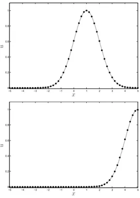
As a comparison, we perform the coordinate space CESE 𝑎-scheme with the range −5 ≤ 𝑥 ≤ 5. In Fig. 2 we show the calculated and analytic solutions at 𝑡 = 1 and at 𝑡 = 5. For the case of 𝑡 = 1, the wave is still wholly inside the numerical region; for the case of 𝑡 = 5, part of the wave has already flowed out of the coordinate space. The NRBC derived from flux conservation automatically gives a smooth leakage of wave through the numerical boundary without causing aliased reflection error.

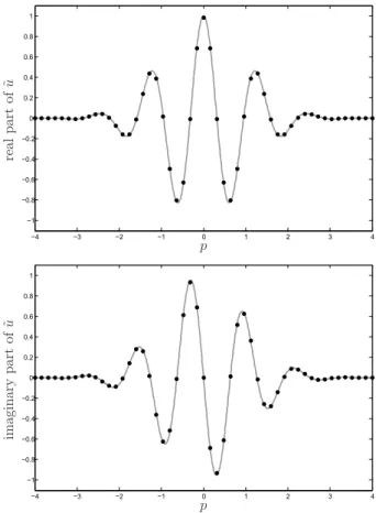
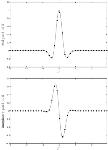
Next we calculate the same wave equation through the developed 𝑎-scheme of the p-CESE method using Δ𝑝 = 0.16, Δ𝑡 = 0.08 and the Courant number 0.5. Fig. 3 shows the real part and the imaginary part of the analytic and computed waves at 𝑡 = 5. Note that ∣˜𝑢(𝑝, 𝑡)∣ = 𝑒−𝑝2₂ _{, thus the momentum space solution at the boundary is equal to 𝑒}−12.5 _{= 3.7 × 10}−6

times of its peak value at 𝑝 = 0, appropriate to be considered as vanishing. Therefore we can take the momentum space wave as stationary with no ﬂow out of the numerical region. The behavior of computational errors will be discussed in the section of KdV equation later, but basically the error is visually invisible. The results of this section imply that for a traveling wave, the momentum space method contains more complete information than the coordinate space method, and the formulation of the new p-CESE method is justiﬁed.

III. CONVECTION-DIFFUSION EQUATIONS Next, we consider the convection-diﬀusion equation :

∂𝑢 ∂𝑡 + 𝑎 ∂𝑢 ∂𝑥 − 𝜇 ∂2_𝑢 ∂𝑥2 = 0, (14)

where the wave velocity 𝑎, and the viscosity coeﬃcient 𝜇 are constants, called the 𝜇-scheme in the CESE framework [1]. By Fourier transformation, Eq. (14) can be transformed into the momentum space form,

∂ ˜𝑢 ∂𝑡 +

(

(17)

Applying the Gauss divergence theorem to the two-dimensional 𝑝 − 𝑡 space, ∮ 𝑆(CE±(𝑗,𝑛)) h ⋅ 𝑑s = − ∫ CE±(𝑗,𝑛) ( 𝑖 𝑎 𝑝 + 𝜇 𝑝2) _{𝑢 𝑑𝑝𝑑𝑡.}_˜ ₍₁₆₎

where h ≡ (ℎ1, ℎ2) = (0, ˜𝑢), we can see that with ˜𝑢 = ˜𝑢(𝑝, 𝑡; 𝑗, 𝑛) deﬁned by Eq. (7), at the mesh points (𝑗, 𝑛), (˜𝑢𝑡)𝑛𝑗 = − ( 𝑖 𝑎 𝑝𝑗 + 𝜇 𝑝2𝑗 ) ˜ 𝑢𝑛 𝑗. (17)

The explicit time-marching scheme is derived similarly to the previous simple wave case, that is, ˜ 𝑢𝑛 𝑗,ℓ± (˜𝑢𝑝¯)𝑛𝑗,ℓ− [ ˜ 𝑢𝑛−12 𝑗±1 2 ∓ (˜𝑢𝑝¯) 𝑛−1 2 𝑗±1 2 ] = −Δ𝑡 2 ( 𝑖 𝑎 𝑝_𝑗±1 4 + 𝜇 𝑝 2 𝑗±1 4 ) ˜ 𝑢∗ ±,ℓ−1, (18)

where ℓ is the iteration index and the iterative scheme is the same as described in the previous section. With the aid of Eqs. (17) and (18), the unknowns ˜𝑢𝑛

𝑗 and (˜𝑢𝑝¯)𝑛𝑗 can be

solved iteratively in terms of known ˜𝑢𝑛−1/2_𝑗±1/2 and (˜𝑢𝑝¯)𝑛−1/2_𝑗±1/2 in the preceding time level. The momentum space convection-diﬀusion equation is also an ordinary diﬀerential equa-tion with the general soluequa-tion

˜

𝑢𝑒(𝑝, 𝑡) = 𝑓 (𝑝) × exp

[

−(𝑖 𝑎 𝑝 + 𝜇 𝑝2)_𝑡]_, ₍₁₉₎

with an arbitrary shape function 𝑓 (𝑝). As a calibration of the p-CESE method, we use a Gaussian shape 𝑓 (𝑝) = exp(−𝑝2_{) below. The numerical results for 𝑎 = 1 and 𝜇 = 1 at} 𝑡 = 5 are depicted in Fig. 4, showing excellent agreements between calculated and exact solutions. As we know, solving Eq. (14) in coordinate space is not as straightforward as this momentum space approach. A 𝑐−scheme with numerical dissipation was implemented for the treatment in the coordinate space approach [2], while the simplest 𝑎−scheme in p-CESE method already gives accurate results. For a reference, the exact solution in coordinate space corresponds to Eq. (19) is

𝑢(𝑥, 𝑡) = √ 𝜋 1 + 𝜇𝑡 × exp [ −(𝑥 − 𝑎𝑡) 4(1 + 𝜇𝑡) ] . (20)

IV. DRIVEN SIMPLE HARMONIC OSCILLATOR

Next we solve a quantum mechanical problem by the p-CESE method. Under the velocity gauge and the dipole approximation, a charge 𝑞 oscillating in the simple harmonic potential

(18)

with applied electromagnetic pulse is described by the time-dependent Schr¨odinger equation 𝑖∂𝑢 ∂𝑡 = [ 𝑝2 2 + 1 2Ω 2_𝑥2_{− 𝐴(𝑡) ⋅ 𝑝} ] 𝑢. (21)

Throughout this section, we use atomic units ¯ℎ = 1, 𝑚 = 1 and 𝑒 = 1, thus 1 a.u. laser peak intensity equals to 7.02 × 1016_{𝑤𝑎𝑡𝑡/𝑐𝑚}2_{. The relationship between electric ﬁeld and} vector potential is given by

𝐸(𝑡) = −∂𝐴(𝑡)/∂𝑡.

The transition probability from the ground state ∣0 > to an excited state ∣𝑁 > is given by Poisson’s distribution [7]

𝑃0→𝑁 = 𝑒−𝜎 𝜎𝑁

𝑁!, (22)

where 𝜎 is a pulse parameter

𝜎 = 1 2Ω ¯ ¯ ¯ ¯ ∫ _∞ ∞ 𝐸(𝑡)𝑒𝑖Ω𝑡_𝑑𝑡 ¯ ¯ ¯ ¯ 2 . (23)

Recast Eq. (21) into p-space, we obtain

𝑖 ˜𝑢𝑡+ 1 2Ω 2_𝑢_˜ 𝑝𝑝= [ 𝑝2 2 − 𝐴(𝑡) ⋅ 𝑝 ] ˜ 𝑢. (24)

With ˜𝑢 = ˜𝑢(𝑝, 𝑡; 𝑗, 𝑛) and expansion of Eq. (7) at mesh point (𝑗, 𝑛), Eq. (24) becomes

(˜𝑢𝑡)𝑛𝑗 = −𝑖 [ 𝑝2 𝑗 2 − 𝐴(𝑡 𝑛_{) ⋅ 𝑝} 𝑗 ] ˜ 𝑢𝑛 𝑗. (25)

Furthermore, for (𝑝, 𝑡) ∈ SE(𝑗, 𝑛) , we deﬁne

h(𝑝, 𝑡; 𝑗, 𝑛) = ( 1 2Ω 2_𝑢_˜ 𝑝(𝑝, 𝑡; 𝑗, 𝑛), 𝑖 ˜𝑢(𝑝, 𝑡; 𝑗, 𝑛) ) , (26)

and the ﬂux theorem for CE±(𝑗, 𝑛) becomes

∮ 𝑆(CE±(𝑗,𝑛)) h ⋅ 𝑑s = ∫ CE±(𝑗,𝑛) [ 𝑝2 2 − 𝐴(𝑡) ⋅ 𝑝 ] ˜ 𝑢 𝑑𝑝𝑑𝑡. (27)

Evaluating the area integral over CE±(𝑗, 𝑛) by the mean value method of ˜𝑢∗± as described

in former sections, we obtain

𝑖{𝑢˜𝑛 𝑗,ℓ± (˜𝑢𝑝¯)𝑛𝑗,ℓ− [ ˜ 𝑢𝑛−12 𝑗±1 2 ∓ (˜𝑢𝑝¯)𝑛− 1 2 𝑗±1 2 ]} ∓ 1 2Ω 2Δ𝑡 Δ𝑝 [ (˜𝑢𝑝)𝑛𝑗,ℓ− (˜𝑢𝑝)𝑛− 1 2 𝑗+1 2 ] = Δ𝑡 2 [ 𝑝2 𝑗±1₄ 2 − 𝐴(𝑡 𝑛−1₄_{) ⋅ 𝑝} 𝑗±1₄ ] × ˜𝑢∗ ±. (28)

(19)

where ℓ is the iteration index, and the iteration scheme as in previous sections is applied for time marching. With the aid of Eqs. (25) and (28), the unknowns ˜𝑢𝑛

𝑗 and (˜𝑢𝑝¯)𝑛𝑗 can be

solved iteratively in terms of the known ˜𝑢𝑛−1/2_𝑗±1/2 and (˜𝑢𝑝¯)𝑛−1/2_𝑗±1/2 of the previous time level. As an illustration of the method, we choose a light pulse with a 𝑆𝑖𝑛2 _envelop,

𝐸(𝑡) = 𝐸𝑚 sin2

𝜋𝑡

𝑇 cos 𝜔𝑡, (29)

0 < 𝑡 < 𝑇.

We assume the carrier frequency of the electric ﬁeld is 𝜔 = 0.057 a.u. (800 nm in wavelength), 𝐸𝑚 = 0.002 a.u., and the total time duration 𝑇 is 8 optical cycles. Furthermore, we assume

the near resonant case, Ω = 0.058 so that excitations are signiﬁcant. The system is initially prepared in the ground state

˜ 𝑢(𝑝, 𝑡 = 0) = 1 (Ω 𝜋)14 exp ( − 𝑝2 2 Ω ) . (30)

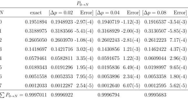
The transition probabilities 𝑃0→𝑁 from the ground state to other excited state 𝑁 are listed in Table I, calculated from the overlap of the ﬁnal wave function ˜𝑢(𝑝, 𝑡 = 𝑇 ) with the eigenstate ˜ 𝑢𝑁 : 𝑃0→𝑁 = ¯ ¯ ¯ ¯ ∫ _∞ −∞ ˜ 𝑢 ˜𝑢∗ 𝑁𝑑𝑝 ¯ ¯ ¯ ¯ 2 . (31)

We can see that reasonably good results are obtained through the p-CESE method, and the error in each transition probability is scaled nearly to (Δ𝑝)2 _{with diﬀerent grids. This error} behavior will be discussed in KdV system.

V. THE KORTEWEG-DE VRIES EQUATION

The Korteweg-de Vries (KdV) equation is a classic example of the nonlinear wave equa-tions [8, 9]. The general form is

1 𝛽 ∂𝑢 ∂𝑡 + 𝛼 𝛾𝑢 ∂𝑢 ∂𝑥 + 1 𝛾3 ∂3_𝑢 ∂𝑥3 = 0, (32)

where 𝛼, 𝛽 and 𝛾 are non-zero constants. The system contains both nonlinearity and dispersion. For convenience, we study in this section the scaled equation

(20)

By Fourier transformation and some manipulations, the momentum space equation is ˜ 𝑢(𝑝, 𝑡)𝑡= 3 𝑖 𝑝 ∫ _∞ −∞ ˜ 𝑢(𝑞, 𝑡) ˜𝑢(𝑝 − 𝑞, 𝑡)𝑑𝑞 + 𝑖 𝑝3_𝑢._˜ ₍₃₄₎

Let h = (0, ˜𝑢) and applying the Gauss divergence theorem in 𝐸2, Eq. (34) becomes ∮ 𝑆(𝑉 ) h ⋅ 𝑑s = ∫ 𝑉 [ 3 𝑖 𝑝 ∫ _∞ −∞ ˜ 𝑢(𝑞, 𝑡) ˜𝑢(𝑝 − 𝑞, 𝑡) 𝑑𝑞 + 𝑖 𝑝3_𝑢_˜ ] 𝑑𝑝𝑑𝑡. (35)

We can see that for a nonlinear system, the source terms on the right-hand side of Eq. (34) contain the convolutional integral of unknown functions, hence the straightforward explicit iteration scheme described in previous sections does not work. We implement two new ideas for the treatment of nonlinear problems in the p-CESE method. First, at each time level, we calculate ˜𝑢(𝑝, 𝑡) and ˜𝑢𝑝(𝑝, 𝑡) at grids of half spacings, instead of spacings at staggered

Δ𝑝 in linear examples. The convolutional integral can then be calculated by Simpson’s rule [10]. Second, for every half-marching time step, say from 𝑡𝑛−1₂ _{to 𝑡}𝑛_{, we begin by using ˜}_𝑢

and ˜𝑢𝑝 at 𝑡𝑛− 1

2 for the source terms and ﬁnd the solution at 𝑡𝑛, then with the obtained, we

can ﬁnd ˜𝑢 and ˜𝑢𝑝 at grids (𝑗 ± 1₄, 𝑛) through the expansion with respect to SE(𝑗, 𝑛) as in

Eqs. (7). These are used in the source terms to generate new solutions iteratively until the convergent criterion is satisﬁed. Usually the results converge within a few iterations.

In mathematical forms, from the conservation laws for CE±(𝑗, 𝑛),

∮ 𝑆(CE±(𝑗,𝑛)) h(𝑥, 𝑡; 𝑗, 𝑛) ⋅ 𝑑s = 3 𝑖𝑝 ∫ CE±(𝑗,𝑛) (∫ _∞ −∞ ˜ 𝑢(𝑞, 𝑡) ˜𝑢(𝑝 − 𝑞, 𝑡) 𝑑𝑞 ) 𝑑𝑝𝑑𝑡 + ∫ CE±(𝑗,𝑛) 𝑖 𝑝3_{𝑢 𝑑𝑝𝑑𝑡,}_˜ (36)

where h(𝑝, 𝑡; 𝑗, 𝑛) = (0, ˜𝑢(𝑝, 𝑡; 𝑗, 𝑛)). We can derive the following 𝑎-scheme iterations

𝑢𝑛 𝑗 = 1 2 { [𝑢 − 𝑢𝑝¯]𝑛− 1 2 𝑗+1₂ + [𝑢 + 𝑢𝑝¯] 𝑛−1₂ 𝑗−1₂ } + 𝐹 Δ𝑝 + 𝐺 Δ𝑝, 𝑢𝑝¯,𝑛𝑗 = 1 2 { [𝑢 − 𝑢𝑝¯]𝑛− 1 2 𝑗+1 2 − [𝑢 + 𝑢𝑝¯]𝑛− 1 2 𝑗−1 2 } + 𝐹 Δ𝑝 − 𝐺 Δ𝑝, (37) where we designate 𝑢𝑛

𝑗 = ˜𝑢(𝑝𝑗, 𝑡𝑛) , 𝑢𝑝¯,𝑛𝑗 ≡ Δ𝑝4 (˜𝑢𝑝)𝑛𝑗, and Δ𝜏 = Δ𝑝2 Δ𝑡2 for shorthand. And

𝐹 = { 3𝑖𝑝𝑖+1/2 ∑ 𝑗 𝑢(𝑝𝑖+1/2− 𝑞𝑗, 𝑡𝑛−1/2)𝑢(𝑞𝑗, 𝑡𝑛−1/2) Δ𝑝 2 + 𝑖𝑝 3 𝑖+1/2𝑢(𝑝𝑖+1/2, 𝑡𝑛−1/2) } Δ𝜏, 𝐺 = { 3𝑖𝑝𝑖−1/2 ∑ 𝑗 𝑢(𝑝𝑖−1/2− 𝑞𝑗, 𝑡𝑛−1/2)𝑢(𝑞𝑗, 𝑡𝑛−1/2) Δ𝑝 2 + 𝑖𝑝 3 𝑖−1/2𝑢(𝑝𝑖−1/2, 𝑡𝑛−1/2) } Δ𝜏.

(21)

The KdV Eq. (33) has a solitonic solution 𝑢(𝑥, 𝑡) = −𝑐 2sech 2₍ √ 𝑐 2 (𝑥 − 𝑐𝑡 + 𝑥0)). (38)

Note that the solution depends on the speed 𝑐 of soliton and therefore multiplying the solution by an arbitrary constant is no longer a solution. Without loss of generality, we set the initial peak position at 𝑥0 = 0 with the wave propagating at speed 𝑐 to the right of the 𝑥-axis without shape change. The exact solution in momentum space is

˜

𝑢𝑒(𝑝, 𝑡) = −𝑝 csch(

𝜋𝑝 √

𝑐) exp(−𝑖 𝑝𝑐𝑡). (39)

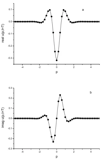
Fig. 5a and 5b depict the real and the imaginary part of the numerical results together with the analytic results at time 𝑡 = 5 and show excellent agreements between the p-CESE calculation and the analytic results.

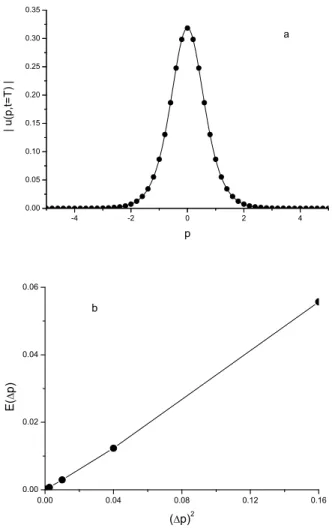
in Fig. 6a, comparison of the magnitudes of the calculated and the exact solutions at 𝑡 = 5 with 𝑐 = 1 is shown. For the soliton solution, although the real part and the imaginary part oscillate with time, the magnitude is stationary as seen from Eq. (39).

The previous section has shown that our developed p-CESE method works well for various kinds of wave problems. Here we present the error analysis for this method. We deﬁne the root-mean-square error at the ﬁnal moment of time as follows :

𝐸(𝑁) = v u u ⎷ 1 𝑁 𝑗=𝑁_∑ 𝑗=0 [𝑢(𝑝𝑗, 𝑡𝑓 𝑖𝑛𝑎𝑙) − 𝑢𝑒𝑥𝑎𝑐𝑡]2. (40)

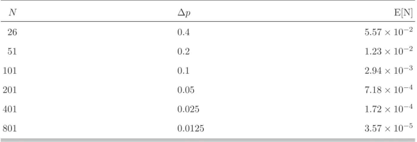
In Table II, we listed the errors with respect to the grid size Δ𝑝 and in Fig. 6b the error versus (Δ𝑝)2 _{are plotted. The straight line shows that the error behaves as ∼ 𝑂(Δ𝑝)}2_{, a} general scaling behavior of our developed p-CESE 𝑎-scheme method.

VI. DISCUSSION AND CONCLUSIONS

In this paper, we developed the CESE method in momentum space on a fundamental scope and explored the solutions of several paradigmatic wave equations, namely the ba-sic one-dimensional wave equation, the convection-diﬀusion equation, the driven quantum mechanical problem and the nonlinear KdV equation. In each problem, we developed an explicit time-marching scheme in the p-CESE method. While it is straightforward for linear

(22)

problems, for nonlinear problems such as the KdV equation, convolution integral of unknown functions in the source term is involved. This difficulty is resolved by employing the half-step grid size for the convolutions and the iterations during time marching. Each system was cal-ibrated with a known exact solution, and we showed that the p-space CESE method works well for systems from classical wave equations, quantum mechanical problems to nonlinear equations, and the error behavior of the developed scheme is ∼ 𝑂(Δ𝑝)2_{. The main} advan-tages of the p-CESE method, in cooperation with the superior CESE method in coordinate space, are threefold. First, like the original CESE method, applying the momentum-time flux conservation concept in staggered mesh, the explicit time marching scheme for every wave equation can be derived. Second, the boundary conditions are fulfilled automatically. That is, for a sufficient large momentum value, the wave and its derivatives are simply van-ishing small at the numerical boundary, because the kinetic energy of a system is physically finite. Third, the information of the wave is completely preserved within the numerical momentum region, without loss at the boundary as in the coordinate space method. This will be especially useful in treating scattering problems. In this paper, we aim to develop a method for waves that extend to far distance as time goes on. This category of problems is closely related to the experimental problems such as photoelectron spectra etc.. The prob-lem with waves extending to far distances is not easy to treat by coordinate space methods, as demonstrated in Fig. 2. We show that the p-CESE is capable for this kind of problem. On the other hand, the boundary value problems in finite domain were solved neatly by coordinate space CESE method [1], and is not our goal here. Our algorithm follows the core scheme of CESE method, and the stability criterion has been rigorously discussed [1, 11]. The criterion in our scheme is 𝑎 𝑑𝑡/𝑑𝑝 ≤ 1. Also, in each time step, we calculate the correla-tion integral and the cost is ∼ 𝑂(𝑁2_{) for 𝑁 grid points. During each time step, there is an} iteration scheme for accurate computation of the correlation integral. However, the integral converges within ten iterations, so the cost is ∼ 𝑐 ⋅ 𝑂(𝑁2_{) where 𝑐 is a constant of order 1.} The computational cost can be compared with other conventional finite-difference schemes. Finally, for realistic problems, higher dimensional method is necessary. This problem, to-gether with higher order of accuracy p-CESE method, is currently under development.

(23)

Acknowledgments

TFJ thanks the support of NSC, Taiwan under the contract of number NSC97-2112-M-009-002-MY3. He also acknowledges the hospitality of NASA/NIA through the MoE between NASA and NARL, Taiwan.

(24)

[1] S.C. Chang and W.M. To, ”A New Numerical Framework for Solving Conservation Laws –

The Method of Space-Time Conservation Element and Solution Element,” NASA/TM 104495

(1991); Chang, S.C. Chang, J. Comput. Phys., 119, 295 (1995).

[2] More details and references can be found in http://www.grc.nasa.gov/WWW/microbus/

[3] S.-C. Chang, A. Himansu, C.-Y. Loh, X.-Y. Wang and S.-T.J. Yu, ”Robust and Simple

Non-Reﬂecting Boundary Conditions for the Euler Equations, A New Approach Based on the Space-Time CE/SE Method, NASA/TMX2003-212495/REV1 (2003).

[4] See for example, Tsin-Fu Jiang and Shih-I Chu, Phys. Rev. A46, 7322 (1992).

[5] U.L. Pen and T.F. Jiang, Phys. Rev. A 46, 4297 (1992); and Phys. Rev. A 53, 623 (1996).

[6] See T.F. Jiang, Comp. Phys. Commun. 178, 571 (2008) and references therein.

[7] C. Cohen-Tannoudji, J. Dupont-Roc, C. Fabre, and G. Grynberg, Phys. Rev. A8, 2747 (1973).

[8] P.G. Drazin and R.S. Johnson, ”Solitons : an Introduction,” (Cambridge Univ. Press, Cam-bridge, 1989).

[9] G.B. Arfken and H.J. Weber, ”Mathematical Methods for Physicists”, 4th Ed. Sec. 8.1 (Aca-demic Press, San Diego, 1995).

[10] J.H. Mathews and K.D. Fink, ”Numerical Methods Using Matlab,” 4th. Ed. Sec. 7.2 (Pearson Prentice Hall, London, 2004).

[11] Sin-Chung Chang, On Space-Time Inversion Invariance and Its Relation to Non-dissipatedness

(25)

TABLE I: Numerical results of transition probability from the ground state to state ∣𝑁 >. Also listed are the exact values and the errors. Three grid spacings Δ𝑝 = 0.08, 0.04 and 0.02 were used in calculations. The time step Δ𝑡 = 8 × 10−4 _{is used throughout.}

𝑃0→𝑁

𝑁 exact [Δ𝑝 = 0.02 Error] [Δ𝑝 = 0.04 Error] [Δ𝑝 = 0.08 Error] 0 0.1951894 0.1948923 -2.97(-4) 0.1940719 -1.12(-3) 0.1916537 -3.54(-3) 1 0.3188975 0.3183566 -5.41(-4) 0.3168929 -2.00(-3) 0.3130507 -5.85(-3) 2 0.2605050 0.2603970 -1.08(-4) 0.2602243 -2.81(-4) 0.2612223 7.17(-4) 3 0.1418697 0.1421716 3.02(-4) 0.1430856 1.21(-3) 0.1462422 4.37(-3) 4 0.0579461 0.0582811 3.35(-4) 0.0591675 1.22(-3) 0.0609044 2.96(-3) 5 0.0189343 0.0191296 1.95(-4) 0.0195836 6.49(-4) 0.0198997 9.65(-4) 6 0.0051558 0.0052353 7.95(-5) 0.0053896 2.34(-4) 0.0053358 1.80(-4) 7 0.0012033 0.0012287 2.54(-5) 0.0012640 6.07(-5) 0.0012595 5.62(-5) ∑ 𝑃0→𝑁 = 0.9997011 0.9996922 0.9996794 0.9995683 noted :_{−2.97(−4) denotes −2.97 × 10}−4 _.

(26)

TABLE II: The root-mean-square error 𝐸[𝑁 ] versus mesh size Δ𝑝 shows 𝑂(Δ𝑝2_{) behavior for KdV}

equation in our p-CESE method under the 𝑎-scheme.

𝑁 Δ𝑝 E[N] 26 0.4 5.57 × 10−2 51 0.2 1.23 × 10−2 101 0.1 2.94 × 10−3 201 0.05 7.18 × 10−4 401 0.025 1.72 × 10−4 801 0.0125 3.57 × 10−5

(27)

n − 1 n −1 2 n n +1 2 n + 1 j − 2 _{j −}3 2 j − 1 j − 1 2 j j + 1 2 j + 1 j + 3 2 j + 2 ∆p/2 ∆t/2 p t ∆p/2 ∆p/2 ∆t/2 ∆t/2 A A A B B C C SE(j, n) (j, n) CE(j, n) (j, n) (j, n) (j −1 2, n − 1 2) (j + 1 2, n − 1 2) CE−(j, n) CE+(j, n) D D D E E F F

(28)

−5 −4 −3 −2 −1 0 1 2 3 4 5 0 0.2 0.4 0.6 0.8 1 x u −5 −4 −3 −2 −1 0 1 2 3 4 5 0 0.2 0.4 0.6 0.8 1 x u

FIG. 2: Results of the coordinate space CESE 𝑎-scheme at 𝑡 = 1 and 5 obtained with 𝑥 ∈ [−5, 5]. Notice that the wave 𝑢 will ﬂow out the boundary at suﬃcient long time. Dots : numerical results.

(29)

−4 −3 −2 −1 0 1 2 3 4 −1 −0.8 −0.6 −0.4 −0.2 0 0.2 0.4 0.6 0.8 1 p re al p ar t of ˜u −4 −3 −2 −1 0 1 2 3 4 −1 −0.8 −0.6 −0.4 −0.2 0 0.2 0.4 0.6 0.8 1 p im ag in ar y p ar t of ˜u

FIG. 3: Computational results ˜𝑢 at 𝑡 = 5 by the p-CESE method. Data obtained with 𝑝 ∈ [−5, 5],

(30)

−3 −2 −1 0 1 2 −0.4 −0.2 0 0.2 0.4 0.6 0.8 1 1.2 p re al p ar t of ˜u −3 −2 −1 0 1 2 −0.8 −0.6 −0.4 −0.2 0 0.2 0.4 0.6 0.8 p im ag in ar y p ar t of ˜u

FIG. 4: Results of ˜𝑢 at 𝑡 = 5 obtained with 𝑝 ∈ [−5, 5] at Δ𝑝 = 0.16, and Δ𝑡 = 0.16. Dots :

(31)

-4 -2 0 2 4 -0.3 -0.2 -0.1 0.0 0.1 r e a l u ( p , t = T ) p a -4 -2 0 2 4 -0.3 -0.2 -0.1 0.0 0.1 0.2 0.3 i m a g u ( p , t = T ) p b

FIG. 5: Results of the real and imaginary part of KdV solution at 𝑡 = 5 obtained with 𝑝 ∈ [−5, 5] and Δ𝑡 = 0.01. Solid line : analytical solution, dots : numerical results.

(32)

-4 -2 0 2 4 0.00 0.05 0.10 0.15 0.20 0.25 0.30 0.35 a | u ( p , t = T ) | p 0.00 0.04 0.08 0.12 0.16 0.00 0.02 0.04 0.06 E ( p ) ( p) 2 b

FIG. 6: a. Results of the magnitude of KdV solution at 𝑡 = 5 obtained with 𝑝 ∈ [−5, 5] and Δ𝑡 = 0.01. Solid line : exact solution, dots : numerical results. b. Error as function of square of grid size Δ𝑝. It shows ∼ 𝑂(Δ𝑝)2 _behavior.

(33)

Adaptive mesh refinement for elliptic interface

problems using the non-conforming immerse

finite element method

Chin-Tien Wu,

∗

Zhilin Li

†

Ming-Chih Lai,

‡

October 30, 2009

Abstract

In this paper, an adaptive mesh refinement technique is developted and analyzed for the non-conforming immersed finite element (IFE) method pro-posed in [25]. The IFE method was developed for solving the second order elliptic boundary value problem with interfaces across which the coefficient may be discontinuous. The IFE method was based on a triangulation that does not need to fit the interface. One of the key ideas of IFE method is to modify the basis functions so that the natural jump conditions are satis-fied across the interface. The IFE method has shown to be order of O(h2₎ and O(h) in L2 _{norm and H}1 _{norm, respectively. In order to develop the} adaptive mesh refinement technique, additional priori and posterior error es-timations are derived in this paper. Our new a priori error estimation shows that the generic constant is only linearly proportional to ratio of the diffusive coefficients β− _{and β}+_{, which improves the corresponding result in [25].}

∗_{Corresponding author. Department of Applied Mathematics, National Chiao-Tung University,}

1001, Ta Hsueh Road, Hsinchu 300, Taiwan. [email protected]

†_{Center for Research in Scientific Computation & Department of Mathematics, North Carolina}

State University, Raleigh, NC. 27695-8205.

‡_{Center of mathematical modeling and Scientific computing, National Chiao-Tung University,}

1001, Ta Hsueh Road, Hsinchu 300, Taiwan.

(34)

We also show that a posteriori error estimate similar to the one obtained by Bernardi and Verf¨urth [4] holds for the IFE solutions. Numerical examples support our theoretical results and show that the adaptive mesh refinement strategy is effective for the IFE approximation.

1 Introduction

The main purpose of this paper is to develop adaptive mesh refinement techniques for the immersed finite element (IFE) method proposed in [25]. Along this line, we also discuss the a priori and a posteriori error estimation for the immersed finite element method. The IFE method was developed for the following interface problem:

−∇ · (β∇u) = f, (x, y) ∈ Ω u |∂Ω = g,

(1)

together with the natural jump conditions on the interface ˜Γ:

[u] |˜_Γ= 0, (2)

[βun] |˜Γ= 0. (3)

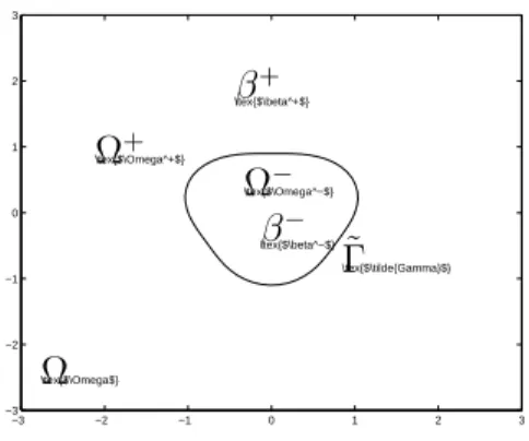
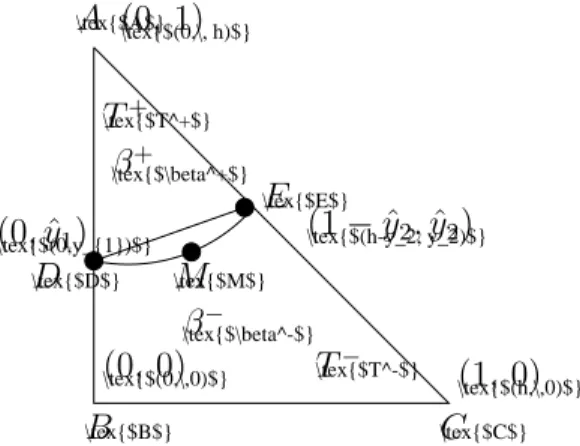
Here, see the sketch in Fig.1, Ω ⊂ R2_{is a convex polygonal domain, the interface} ˜

Γ is a curve separating Ω into two sub-domains Ω−_{, Ω}+_{such that Ω = Ω}−_∪Ω+_∪˜_Γ, and the coefficient β(x, y) is a piecewise constant function defined by

β(x, y) = ½

β−_{, (x, y) ∈ Ω}−_,

β+_{, (x, y) ∈ Ω}+_.

The interface problem considered here appears in many engineering and sci-ence applications. The immersed finite element (IFE) space was first introduced in [25], in which some preliminary analysis and numerical results are reported, and has been shown its capability on handling interface problems with nonho-mogeneous interface jump conditions [with a nonzero constant value on the right hand of (2) and/or (3)] by either simply modifying the IFE space or reducing the interface problem to a new problem with homogeneous interface jump conditions

(35)

−3 −2 −1 0 1 2 3 −3 −2 −1 0 1 2 3 \tex{$\tilde{Gamma}$} \tex{$\beta^+$} \tex{$\beta^−$} \tex{$\Omega$} \tex{$\Omega^+$} \tex{$\Omega^−$} ˜ Γ β+ β− Ω Ω+ Ω−

Figure 1: A rectangular domain Ω = Ω+_{∪ Ω}−_{with an immersed interface ˜}_{Γ. The}

coefficients β(x) may have a jump across the interface.

via the usual homogenization technique based on a change of variable [23]. Some related work can be found in [?, 18, 19, 26].

The basic idea of the immersed finite elements is to form a partition =h

in-dependent of interface ˜Γ so that partitions with simple regular structures can be used to solve an interface problem with a rather complicated or varying interface. Obviously, triangles in a partition can be separated into two classes:

• Non-interface triangles: The interface ˜Γ either does not intersect with this triangle, or it intersects with this triangle but does not separate its interior into two nontrivial subsets.

• Interface triangles: The interface ˜Γ cuts through its interior.

In a non-interface triangle, the standard linear polynomials is employed as local basis functions. However, in an interface triangle, a piecewise linear polynomial is defined in the two subsets formed by the interface in a way that the functions satisfy the natural jump conditions (either exactly or approximately) on the in-terface and retain specified values at the vertices of the inin-terface triangle. The immersed finite element space defined over the whole domain Ω can then be con-structed through the standard finite element assembling procedure. We refer the readers to [?, 9–11, 14, 17, 22, 24] for more background materials about immersed interface and immersed finite element methods as well as their applications.

(36)

Without loss of generality, we assume that the triangles in the partition have the following features:

(H1): If ˜Γ meets one edge of a triangle at more than two points, then the edge is part of ˜Γ.

(H2): If ˜Γ meets a triangle at two points, then these two points must be on different edges for this triangle.

In order to obtain error estimates, we assume that the underlying mesh is fine enough such that the interface can be approximated by a line segment with a small perturbation in a magnitude of O(h2_{). Furthermore, the source function f and the} interface ˜Γ are assumed to be smooth enough such that the weak solution of the problem (1) can be approximated by a piecewise C2_{function. These requirements} lead to our third hypothesis:

(H3): The segment of the interface ˜Γ in a triangle T ∈ =h is defined by a

piecewise C2_{function and the function space C}2_{(T ) is dense in H}2_{(T ).}

It is well known that the standard finite element method (FE) with linear finite elements can be used to solve such elliptic interface problems [see [3, 5, 6] and the references therein]. However, in order to achieve the optimal O(h2_{) accuracy} in the numerical solutions, an interface fitted grid is needed. In applications with nontrivial interfaces or the time-varying interfaces, this restriction prevents the Galerkin method with linear finite elements from working efficiently since mesh moving or re-meshing is required. On the other hand, although the mesh moving and re-meshing may produce extra technical difficulties and computation over-head for the standard FE method, the standard FE method has a great advantage on increasing the accuracy of the numerical solutions at low cost through the adaptive mesh refinement process. In the adaptive mesh refinement process, first an error indicator ηT used to pin point the locations with large error is computed on each

element in a given triangulation. Second, the elements in which the error indicator has large value are marked for refinement according to a given marking strategy. A heuristic marking strategy is the maximum marking strategy where an element T∗

will be marked for refinement if ηT∗ > θ max_{T ∈=}_hη_T, with a prescribed threshold

0 ≤ θ ≤ 1. Some other marking strategies can also be seen in [13]. Finally, the marked triangles are divided into sub-triangles by rules such as the regular

(37)

refinement algorithm or the longest side bisection algorithm [15] [16]. An ap-proximate solution is then computed on the refined mesh. The above procedure can be repeatedly applied until the accuracy of the approximated solution is sat-isfied. The theoretical foundation of the mesh refinement strategy is based on the a posteriori error estimation proposed by Babuˇska and Rheinboldt [1] and further developed by many researchers such as Zienkiewicz [27], Bank and Weiser [2], and Verf¨urth [20, 21]. The convergence of the adaptive mesh refinement process has been shown by Morin, Nochetto and Siebert [12].

It has been shown that the IFE interpolation errors on a uniform fixed (such as Cartesian) partition is of the order of O(h) in the H1 _{norm and of the order of} O(h2_{) in the L}∞ _{and L}2 _{norms under the hypothesis (H}

1), (H2) and (H3) [26]. In this work, we obtain the same order of the error estimations and further show that the generic constants in these estimations are linearly proportional to the ratio max

n ρ,1

ρ

o

of the diffusion coefficients, here ρ = β_β−+. The a posteriori

esti-mations of the finite element solutions mentioned above are obtained mostly on fitted grids. Recently, A. Hansbo and P. Hansbo propose an unfitted finite element method for the elliptic interface problem. The same order of a priori error esti-mations is obtained and an a posteriori estimator is proposed [8]. Here, we also derive an a posteriori error estimation for the IFE method based on the methodol-ogy developed by Verf¨urth [4]. Our numerical results support the effectiveness of the proposed a posteriori error estimation.

This paper is organized as follows. In section 2, we show the existence and uniqueness of the element IFE basis function and derive some auxiliary inequal-ities that are needed for the error estimation in section 3. We derive the a priori error estimations and the a posteriori error estimation in section 3 and present our numerical results in section 4. Finally, we draw our conclusions in section 5.

2 Review of the immersed finite element space

First we present a brief review of the immersed finite element space and the con-struction of the basis functions.

Given a regular mesh =h on the domain Ω, let T be an interface triangle in

(38)

=h with vertices A, B and C where the interface passes through the interior of

T and intersect with the edges of T at points D and E. Let ˜ΓT = ˜Γ ∩ T . In the

immersed finite element method, the interface ˜ΓT is commonly approximated by

the line segment DE, denoted by ΓT. The formulation of the immersed finite

element method follows the idea that similar to the Hsieh-Clough-Tocher macro element [7] in which the piecewise polynomial in each element is required to satisfy certain constrains to ensure the C1_{-continuity on the whole domain. The} immersed finite element space on a triangle T, denoted by SI

h(T ), is the linear

space of all piecewise linear functions that satisfy the continuity condition [φ]ΓT =

0 and the homogeneous flux jump condition [β∂nφ]ΓT = 0 on the approximate

interface ΓT. Assume the element basis functions on the reference triangle have

the following form:

φ+= a0+ a1x + a2y for (x, y) ∈ T+ φ− _{= b}

0+ b1x + b2y for (x, y) ∈ T−.

It has been shown that the coefficients ai and bi, i = 1 · · · 3, can be determined

uniquely. In [25], the continuity condition [φ]ΓT = 0 is satisfied by enforcing

the continuity on the intersection points D and E, i.e., φ+_{(D) = φ}−_{(D) and}

φ+_{(E) = φ}−_{(E). In this work, we replace the condition φ}+_{(E) = φ}−_{(E) by}

~t · Oφ+ _{= ~t · Oφ}−_{, here ~t is the unit tangent of the approximated interface Γ} T.

The existence and uniqueness of the immersed finite element basis functions are reassured in the following theorem. The interpolation errors in the L∞_{, L}2 _and H1 _{norms will be estimated in the next section.}

Theorem 2.1 Let T denote a triangle with vertices (xi, yi), i = 1 · · · 3 in a given

uniform mesh, the associated IFE basis functions φ ∈ SI

h(T ) consisting of φ+

and φ− _{on the reference triangle are uniquely determined by the nodal values}

φ(xi, yi), i = 1 · · · 3.

Proof: Let Φ be the affine transformation that maps the reference triangle to the triangle T via Φ(0, 0) = (x1, y1), Φ(1, 0) = (x2, y2) and Φ(0, 1) = (x3, y3). Let φ(xi, yi) = φi, i = 1 · · · 3. From the nodal values and the continuity at

(39)

\tex{$A$} \tex{$B$} \tex{$C$} \tex{$E$} \tex{$D$} \tex{$(h,\,0)$} \tex{$(h-y_2, y_2)$} \tex{$(0,\,0)$} \tex{$(0,y_{1})$} \tex{$(0,\, h)$} \tex{$\beta^+$} \tex{$\beta^-$} \tex{$T^+$} \tex{$T^-$} \tex{$M$} A B C E D (1, 0) (1 − ˆy2, ˆy2) (0, 0) (0, ˆy1) (0, 1) β+ β− T+ T− M

Figure 2: A typical triangle element with an interface cutting through. The arc DME is part of the interface curve ˜Γ which is approximated by the line segment DE. In this picture, T is the triangle 4ABC, T+ _{= 4ADE, T}− _{= T − T}+_{, and} T∗ _{is the region enclosed by the DE and ˜}_Γ.

node D, we have

φ3 = φ+(0, 1) = a0+ a2 ⇒ a0 = φ3− a2 (4)

φ1 = φ−(0, 0) = b0 (5)

φ2 = φ−(1, 0) = b0+ b1 ⇒ b1 = φ2− φ1 (6)

a0+ a2yˆ1 = b0+ b2yˆ1. (7)

Plugging equations (4) and (5) into equation (7) implies

(−1 + ˆy1)a2− ˆy1b2 = φ1− φ3. (8) Moreover, from the flux continuity condition and the continuity of the solution along the tangential direction of the interface, we have

(

~n(Φ−1₎T_Oφ+_{= ρ~n(Φ}−1₎T_∇φ−

~t(Φ−1₎T_Oφ+_{= ~t(Φ}−1₎T_Oφ−_, (9)

where n = (n1, n2) and t = (−n2, n1) are the normal and tangent vectors of the interface respectively, and ρ = β_β−+. Let (m1, m2) = ~n(Φ−1)T and (m3, m4) =

~t(Φ−1₎T_{. The two equations in (9) can be rewritten as following:}

m1a1+ m2a2− ρm2b2 = −ρm1φ1+ ρm1φ2 (10) m3a1+ m4a2 = m3(φ2 − φ1) + m4b2. (11)

(40)

Plugging (8) into (10) and (11) and writing the resulted equations in the matrix form, we have · m1yˆ1 m2(ˆy1+ ρ(1 − ˆy1)) m3yˆ1 m4 ¸ · a1 a2 ¸ = · (−ρm2− ρm1yˆ1) ρm1yˆ1 ρm2 −m4− m3yˆ1 m3yˆ1 m4 ¸  φ1 φ2 φ3   = · ρm1yˆ1 ρm2 m3yˆ1 m4 ¸ · φ2− φ1 φ3− φ1 ¸ . (12)

To prove the theorem, we only need to show the metric

A = · m1yˆ1 m2(ˆy1+ ρ(1 − ˆy1)) m3yˆ1 m4 ¸ is non-singular. Let ρ∗ _{= ˆ}_y

1+ ρ(1 − ˆy1). We can see clearly that ρ∗ ≥ 1 when ρ ≥ 1 and 0 ≤ ρ∗ _{≤ 1 when ρ ≤ 1. Since m}

1m4 − m2m3 = det(Φ) > 0, m2m3 < 0 and m1m4 > 0, we have

det(A) = ˆy1((m1m4− m2m3) − (ρ∗− 1)m2m3) > 0, if ρ ≥ 1 (13) and

det(A) = m1m4(1 − ρ∗)ˆy1+ ρ∗yˆ1(m1m4− m2m3) > 0, if 0 < ρ < 1. (14) Now from (13) and (14), we can conclude the matrix A is nonsingular and the theorem holds.¤

Remark 2.2 We can further estimate

det(A) = ˆy1(h−2+ (ρ∗− 1)ny2) = h−2(ˆy1ρ∗)

= h−2(ˆy1(ˆy1+ ρ(1 − ˆy1))) > min{1, ρ}h−2yˆ1, for ρ > 1, and det(A) = h−2_y_ˆ

1 > ˆy1h−2min{1, ρ}, for 0 ≤ ρ ≤ 1,

from the equations (13) and (14), respectively. Therefore, the following estimation of det(A) holds

det(A) ≥ ˆy1h−2min{1, ρ}. (15)

(41)

Moreover, Let ∆φ1 = φ2− φ1, ∆φ2 = φ3− φ1, and B = · ρm1yˆ1 ρm2 m3yˆ1 m4 ¸ . The equation (12) implies

· a1− ∆φ1 a2− ∆φ2 ¸ = A−1(B − A) · ∆φ1 ∆φ2 ¸ (16) = yˆ1(ρ − 1) det (A) · m2m4 m2m4 −ˆy1m2m3 −ˆy1m2m3 ¸ · ∆φ1 ∆φ2 ¸ . Also, from the equations (6), (8), and (16), we have

· b1 − ∆φ1 b2 − ∆φ2 ¸ = " 0 ˆ y1−1 ˆ y1 (a2− ∆φ2) # (17) = yˆ1(ˆy1− 1)(ρ − 1) det (A) · 0 0 −m2m3 −m2m3 ¸ · ∆φ1 ∆φ2 ¸

By applying the estimation (15) to the equations (16) and (17), we can easily show that the following inequalities hold:

° ° ° ° µ a2− ∆φ1 a3− ∆φ2 ¶°_° ° ° ∞ ≤ c+_max{ρ,1 ρ} ° ° ° ° µ ∆φ1 ∆φ2 ¶°_° ° ° ∞ , ° ° ° ° µ b2− ∆φ1 b3− ∆φ2 ¶°_° ° ° ∞ ≤ c−_max{ρ,1 ρ} ° ° ° ° µ ∆φ1 ∆φ2 ¶°_° ° ° ∞ , (18)

where c+ _{and c}−_{are constants independent with ρ.}

3 The priori and posteriori error estimations

In this section, we define the IFE solution of the interface problem (1) and derive the priori and posteriori error estimations of the IFE solution. We first introduce some notations in the following:

• Let =h denote the regular mesh that satisfies the usual admissibility and the

shape regularity. Let ˘=h be the set of elements intersect with the interface,

(42)

and=◦h= =h\ ˘=h. For τ ∈ =h, let ∂τ denote the set of boundary segments

of the element τ and Eh = ∪τ ∈=h∂τ . Let ˘Eh be the set of edges intersect

with the interface and E◦h = Eh\ ˘Eh. Moreover, Nh = the set of all vertices

in =h, Nτ = vertices of an element τ and Ne = vertices of an edge e ∈ Eh.

Also, for any element τ ∈ =h, edge e ∈ E and node z ∈ Nh, let

ωτ = [ τ0_{∩τ ∈∂τ} τ0_{, ˜}_ω τ = [ τ0_{∩τ 6=ø} τ0_{, ω} e= [ Nτ∩Ne6=ø0 τ0_{, ω} z = [ z∈τ0 τ0

• We denote by H0 _{and H}k_{, the usual Lebesgue L}2_{-integrable space and} the Sobolev spaces equipped with the standard norms kf k_k for f ∈ Hk_,

k = 0 · · · 2. The notations kf k_k,Ω₀, k = 0 · · · 2, and kf k_β,Ω₀ denote the usual Sobolev norms and the energy norm of f on a sub-domain Ω0 ⊂ Ω. The piecewise linear polynomial space on a sub-domain Ω0 is denoted by Sh(Ω0). The immersed finite element space on the domain Ω, is denoted by SI

h(Ω), is defined by ShI(Ω) =

©

φ | φ|τ ∈ ShI(τ ), for all τ ∈ =h, and

φ|τ(z) = φ|τ0(z), for z ∈ N_τ ∩ N_τ0}. The notation S_h,0I (Ω) denote the

sub-space in SI

h(Ω) with homogeneous boundary condition, {φ ∈ ShI(Ω) | φ|∂Ω =

0}.

• For each vertex z ∈ Nh, let ϕzdenote the linear nodal basis function. With

every element τ and every edge e, we associate the bubble functions ψτ =

27Q_z∈N_τϕz and ψe = 4

Q

z∈Neϕz. Let In denote the nodal interpolant,

πz denote the L2 orthogonal projection onto the piecewise linear function

space in ωz, and Iπ denote the quasi-interpolant of a function u defined as

Iπu =

P

z∈=h(πzu)ϕz.

For any function φ ∈ H1_{(Ω), the IFE interpolant of φ is denoted by φ}

I ∈ ShI

that satisfies ϕzφI = φ(z) for all z ∈ Nh. The IFE solution of problem (1) denoted

by uI

hsatisfies the standard variation formulation of (1) as following:

(βOν , OuI_h) = (ν , f ), for all ν ∈ SI h,0(Ω),

where (· , ·) is the usual inner product in the H0_{(Ω). To derive the a priori error} estimations of °°u − uI h ° ° 0 and ° °u − uI h ° °

1, we need to estimate the interpolation errors of φ − φI for any φ ∈ H1(Ω) ∩ C(Ω), here φI ∈ ShI(T ) denote the IFE

(43)

interpolant of φ. In the following theorem, we first estimate the errors of φ − φI

and Oφ − OφI in the L∞norm.

Theorem 3.1 Let T be a triangle in a uniform mesh =h and the interface ˜Γ

sat-isfies the hypothesis (H1), (H2) and (H3). Let ΓT denote the line segment that

approximates ˜ΓT. Let φ be an arbitrary function in C2(T ) and φI ∈ ShI(T ) be the

IFE interpolant of φ. The following error estimates hold. kOφ(x, y) − OφI(x, y)k∞,T ≤

( ch kD2_φk ∞,T when (x, y) ∈ Ω\T∗ c kD2_φk ∞,T when (x, y) ∈ T∗ (19) kφ(x, y) − φI(x, y)k∞,T ≤ ch2 ° °D2_φ°° ∞,T, (20) where c = O(max{1 ρ, ρ}) and T

∗ _{is the region enclosed by ˜}_Γ

T and ΓT.

Proof: First, we estimate the error of Oφ − OφIat element nodal points of the

reference triangle in the following: From the Taylor expansion of φ, we have

φ+_(ˆ_{x, ˆ}_{y) = φ}+_{(0, 1) + Oφ}+_{(0, 1)} · ˆ x ˆ y − 1 ¸ + e1 (21) φ−_(ˆ_{x, ˆ}_{y) = φ}−_{(0, 0) + Oφ}−_{(0, 0)} · ˆ x ˆ y ¸ + e2, (22)

where e1 ≤ (ˆy1−1)(kD2φk_∞(ˆy1−1)h2) and e2 ≤ ˆy1kD2φk_∞yˆ1h2, and |e2− e1| ≤ 2 maxv∈{|ˆy1|,|ˆy1−1|}{vT kD2φk_∞v}h2. By imposing the continuity at node D, from

(21) and (22), we have

φ(0, ˆy1) = φ+(0, 1) + φ+yˆ(0, 1)(ˆy1− 1) + e1 = φ−_{(0, 0) + φ}−

ˆ

y(0, 0)(ˆy1) + e2. The above equation implies

(−1 + ˆy1)φ+yˆ(0, 1) − ˆy1φy−ˆ(0, 0) = φ1− φ3+ e2− e1. (23) Next, from the flux continuity and tangential continuity on the interface, we have

m1φ+xˆ + m2φ+yˆ = ρ(m1φ−xˆ + m2φ−yˆ) m3φ+xˆ + m4φ+yˆ = m3φ−xˆ + m4φ−yˆ.

(24)

多重網格法與保結構二次特徵值問題計算對預測壓電材料裂縫成長的重要性

行政院國家科學委員會專題研究計畫 成果報告

多重網格法與保結構二次特徵值問題計算對預測壓電材料

裂縫成長的重要性

研究成果報告(精簡版)

中 華 民 國 98 年 10 月 30 日

I.

introduction:

θ

βθ

θ

θ

θ π

π

( )

(

)

( )

(

)

II.

Multigrid algorithm:

υ

υ

III.

Errors for each studied case over different meshes

π

θ

π

θ

π

θ

π

θ

π

θ

π

θ

π

θ

π

θ

Multigrid convergence

π

θ

π

θ

π

θ

π

θ

π

θ

π

θ

π

θ

π

θ

π

θ

π

θ

π

θ

π

θ

Momentum-time ﬂux conservation method for one-dimensional

wave equations

Abstract

Adaptive mesh refinement for elliptic interface

problems using the non-conforming immerse

finite element method

Chin-Tien Wu,

Zhilin Li

Ming-Chih Lai,

October 30, 2009

1 Introduction

2 Review of the immersed finite element space

3

行政院國家科學委員會專題研究計畫成果報告

中華民國 98 年 10 月 30 日

_π