國
立
交
通
大
學
資訊科學與工程研究所
碩
士
論
文
在多核心嵌入式平台使用平行處理加速 H.264 視訊解碼
Parallelization of H.264 video decoder for Embedded Multicore
Processor
研 究 生:陳彥廷 Student:Yan-Ting Chen
指導教授:蔡淳仁 Advisor:Chun-Jen Tsai
在多核心嵌入式平台使用平行處理加速 H.264 視訊解碼
Parallelization of H.264 video decoder for Embedded Multicore
processor
研 究 生:陳彥廷 Student:Yan-Ting Chen
指導教授:蔡淳仁 Advisor:Chun-Jen Tasi
國 立 交 通 大 學
資 訊 科 學 與 工 程 研 究 所
碩 士 論 文
A ThesisSubmitted to Institute of Computer Science and Engineering College of Computer Science
National Chiao Tung University in partial Fulfillment of the Requirements
for the Degree of Master
in
Computer Science
July 2014
Hsinchu, Taiwan, Republic of China
I
中文摘要
本論文主旨在於在多核心平台上對 Baseline H.264/AVC decoder 用不同的平行化 方式達到加速的效果,並分析 data parallelism 與 task parallelism 的平行技術,如 static scheduling 與 dynamic scheduling、static partition 與 dynamic partition、task buffer monitoring 等等,並探討平行化過程中所產生的負擔與問題,如資料的搬移、記憶體 使用率、synchronization、load balancing 議題等等,以上的平行視訊解碼設計及分析 是在一個新的應用處理器架構上進行[14]。這個新的多核心處理器架構可以在不增加 額外 system bus 負擔下,採用工作切割精細的 software-pipeline 平行化方式,來增加 pipeline-based video decoder 的效能,根據我們實驗的結果,採用 dynamic pipeline partition 在三顆核心下能相對於單核心 H.264/AVC 解碼器有接近三倍的加速。
II
Abstract
In this thesis, we present two parallel decoding approaches to enhance the performance of H.264/AVC decoders on multiprocessor platform. We analyze data-level parallelism and task-level parallelism for various parallel decoding techniques, such as static and dynamic scheduling, static and dynamic partitioning or FIFO task buffers monitoring etc. We discuss some overheads and problems resulted from the parallelization process, such as data transfer, memory usage, synchronization, or load balancing issue etc. The investigation of parallel video decoding is conducted on a new multicore application processor architecture that facilitates the adoption of the fine-granularity software-pipeline parallelism without causing extra burden on the system bus and it will increase pipeline-based video decoder performance. Experimental results show that the adoption of the dynamic pipeline partition approach could nearly be three times faster than a single-core H.264/AVC decoder does.
III
誌謝
這篇論文能夠順利完成,最需要感謝的就是蔡淳仁老師,每次研究遇到瓶頸時, 老師總是耐心的提點,而每次在與老師討論的過程中,總是能獲益良多,而且也讓我 見識到何謂是嚴謹的推演、以及對數據的敏感,也謝謝老師總是能分享在業界的經驗 以及小技巧。在這裡也感謝實驗室的各個同學,謝謝他們總是能分享各種經驗,讓許 多事情能順利的完成,也消磨了不少研究所單調的日子。接下來要感謝父母支持我完 成碩士學位,而因為有大家的支持,才能成就今日的我,我也才能順利的完成論文、 並且畢業。IV
章節目錄
一、緒論 ... 1 1.1 簡介 ... 1 1.2 論文架構 ... 2 二、H.264/AVC ... 3 2.1 H.264/AVC 壓縮標準概論 ... 3 2.1.1 Profile ... 4 2.1.2 H.264/AVC 影像格式階層架構 ... 5 2.2 H.264/AVC 核心技術 ... 7 2.3 熵編碼(Entropy) ... 82.4 Inverse Transform and Inverse Quantization... 10
2.5 Intra Prediction ... 12
2.6 Inter Prediction ... 14
2.6.1 Sub-pixel interpolation ... 16
2.7 In-loop Filter ... 18
2.8 Google Android’s H.264/AVC baseline decoder ... 19
三、Introduction to Parallel H.264 Decoding Scheme ... 20
3.1 Related Work ... 20
3.2 Macroblock dependencies of H.264/AVC ... 22
3.3 Data-level Parallelism ... 24
3.3.1 DLP Overview ... 24
3.3.2 Static scheduling 實作與技術 ... 26
四、Proposed Parallel H.264 Decoder Scheme ... 30
4.1 TLP Overview ... 30
V
4.3 Memory usage of parallel H.264/AVC video decoding ... 43
五、實驗結果 ... 47
5.1 Xilinx XUPV5-LX110T development board ... 47
5.1.2 Application Processor Soc 架構 ... 49
5.1.3 The IPC controller ... 52
5.1.4 Software kernel and Synchronization Schemes... 53
5.2 NEXUS 7 (2013 版)平台 ... 55
5.3 測試環境 ... 56
5.4 實驗數據與探討 ... 58
六、結論與未來展望 ... 67
參考文獻 ... 69
附錄 A:Speedup ratio of different cache size ... 72
附錄 B:Macroblock Mode Distributions and Performance (Detail version) ... 73
附錄 C:PAC Duo Platform ... 74
C.1、摘要 ... 74
C.2、系統架構 ... 74
C.2.1 PAC 系統架構 ... 74
C.3、Software Pipeline 實作 ... 79
C.3.3 Pipeline stage partition ... 81
C.4、實驗結果 ... 82
C.4.1 Impact of MB type distribution... 82
C.4.2 Impact of circular buffer depth ... 83
VI
List of Figures
Figure 1. Chronological Table of Video Coding Standards 3
Figure 2. H.264/AVC 分層圖 4
Figure 3. H.264 Profile 5
Figure 4. H.264/AVC Slice and MB 6
Figure 5. H.264 syntax 6
Figure 6. H.264/AVC Baseline Deocder 7
Figure 7. Exp-Golomb code table 8
Figure 8. Zig-Zag order scan 9
Figure 9. Transform formulas 10
Figure 10. DCT formulas 10
Figure 11. Transformation and Quantization 11
Figure 12. Intra 4x4 modes and their directions 12
Figure 13. Intra 16x16 modes and their directions 13
Figure 14. Sample sequence 14
Figure 15. Partition of macroblock and sub-block 14
Figure 16. Inter Prediction 15
Figure 17. Full-pixel samples (shaded blocks with upper-case letters) and sub-pixel sample positions (un-shaded blocks with lower-case letters) fro
quarter-pixel sample luma interpolation 16
Figure 18. Sub-pixel sample position a in chroma interpolation and surrounding
full-pixel position samples A, B, C, and D 17
Figure 19. Determining the boundary strength 18
Figure 20. In-loop filter 流程圖 18
VII
Figure 22. Android Media Framwork 19
Figure 23. Dependencies of H.264/AVC 23
Figure 24. Data dependency neighborhood of the MB decoding process 23
Figure 25. Data-level Parallelism 24
Figure 26. Exploiting MB parallelism in the spatial domain. 25
Figure 27. DLP- Flow chart 26
Figure 28. The Single-row splitting approach 26
Figure 29. Example of the Single-row splitting approach 27
Figure 30. Two different entropy decoding schemes 28
Figure 31. Task-level Parallelism 32
Figure 32. The decoding steps of an I-MB and a P-MB of H.264/AVC 32
Figure 33. Static pipeline partitioning for the P-MBs and I-MBs of H.264/AVC 34 Figure 34. (a) ~ (b) Two kinds of different partition for dynamic pipeline
partitioning using MB mode 36
Figure 35.Top: the speedup ratio of the dynamic (use MB type) and static
pipeline partition decoder for [email protected]. Bottom:bits per frame of the
video sequence 37
Figure 36. Top: the speedup ratios of the dynamic (use MB type) and static pipeline partition decoder for [email protected]:bits per frame of the
video sequence 37
Figure 37. Top: the speedup ratio of the dynamic and static pipeline partition
decoder for [email protected]. Bottom: the number of the I4x4 MBs 38 Figure 38. Top: the speedup ratio of the dynamic and static pipeline partition
decoder for Stefan@512kbps. Bottom: the number of the Skip MBs 38 Figure 39. The runtime buffer growth at frame #1 of the Stefan@512kbps for the
VIII
static and dynamic (skip) partition pipeline decoder 39
Figure 40. The runtime buffer growth at frame #152 of the [email protected] for
the static and dynamic (skip) partition pipeline decoder 40
Figure 41.The rule for dynamic partition using monitoring buffer 41
Figure 42. The decoding steps for dynamic partition pipeline decoder using
monitoring buffer 41
Figure 43. The runtime buffer growth at frame #152 of the [email protected] for the dynamic#1 (use skip) and dynamic#2 (monitor) partition pipeline
decoder 42
Figure 44. The count of repeated reference pixel for [email protected] 44 Figure 45. The count of repeated reference pixel for crew@512kbps 44
Figure 46. The count of repeated reference pixel for new@15mbps 45
Figure 47. The count of repeated reference pixel for news@512kbps 45
Figure 48.Xilinx XUPV5-LX110T Evaluation Platform 48
Figure 49.Proposed architecture on a Xilinx Virtex-5 FPGA錯誤! 尚未定義書籤。
Figure 50. Stage k 之 IPC controller 架構圖 52
Figure 51. The memory map of the system on an FPGA development boad 53 Figure 52. Pseudo code that performs stage k operations in pipeline datapath 54
Figure 53. NEXUS 7 (2013) platform 55
Figure 54. PAC Duo 開發板 75
Figure 55. PAC Duo SoC 晶片 75
Figure 56. PAC Duo SoC 系統架構圖 76
Figure 57. PAC DSP 系統架構圖 78
Figure 58. PAC DSP 指令封裝格式 78
IX
Figure 60. The proposed software pipeline architecture for the H.264/AVC
decoder 80
Figure 61. Overlapping of each core's operations. The subscripts are MB number 81
Figure 62. 各模組時間分佈 81
X
List of Tables
Table 1. The interplation filters and reference data size of one MxN luma
partition of single direction... 17
Table 2. Maximum parallel MBs for several resolutions using DLP ... 25
Table 3. Macroblock mode distributions and performance (use static pipeline partitioning) ... 35
Table 4. The count of Integer MV and Non-Integer MV... 46
Table 5. Memory access ratio of each H.264/AVC decoder module (W: frame width, H: frame height) ... 46
Table 6. FPGA LOGIC USAGE OF THE PROPOSED ARCHITECTURE ... 51
Table 7. The information contained in video sequences... 56
Table 8. Baseline Single-Core Video Decoder Performance ... 59
Table 9. Proposed Static Pipeline Partition Decoder Performance... 59
Table 10. Proposed Dynamic Pipeline Partition Decoder (use MB mode) Performance ... 60
Table 11. Proposed Dynamic Pipeline Partition Decoder (monitoring buffer) Performance ... 60
Table 12. DRAM-BASED Three-Core Pipeline Decoder Performance ... 61
Table 13. Wavefront Three-Core Decoder Performance ... 61
Table 14. Speedup Ratio of Different Decoders at 512 kbps ... 64
Table 15. Speedup Ratio of Different Decoders at 1.5mbps ... 64
Table 16. Speedup Ratio Wavefront with Interleaved Entropy Decoder ... 65
Table 17. Speedup Ratio for crew 720x480 video sequence ... 65
Table 18. Speedup Ratio of Wavefront Decoder on NEXUS 7 2013 ... 66 Table 19. Comparisons of parallelization in various H.264/AVC Wavefront
XI
Decoder ... 66
Table 20. SPEEDUP RATIO OF DIFFERENCE DECODERS AT 512 KBPS ... 72
Table 21. SPEEDUP RATIO OF DIFFERENCE DEOCDERS AT 1.5 MBPS ... 72
Table 22. Distribution of the MB types ... 82
1
一、緒論
1.1 簡介
隨著 3C 技術的整合與網際網路的蓬勃發展,嵌入式系統被視為是未來科技應用 的主軸,而與我們生活息息相關的是以嵌入式系統為主的資訊家電,如智慧型手 機、數位隨身聽、數位相機、平板電腦、遊戲機等等,其中以智慧型手持式裝置滲 透率最高,未來成長最具有潛力,而手持式裝置的功能也已經從單純收發簡訊及電 話通訊轉為現今的視訊通話、高清影片播放和進行高特效遊戲等等的強大功能,智 慧型手持裝置可以被視為一台縮小版的桌上型電腦。近年來網路興盛,3G、4G 技 術興起,網路速度飛躍性的成長,這意味著手持式裝置能在極短的時間內接收大量 的資料,因此嵌入式系統將需要提供更強大的運算能力來因應使用者需求。 而在嵌入式系統各種應用中,多媒體應用往往是嵌入式系統設計中的一大重點, 因為多媒體應用是最直接與使用者進行互動,且多媒體程式其優劣能容易被使用者 在視覺或聽覺上感受到,要能提供使用者感受到平順的影音同步播放,就必須在短 時間內處理大量多媒體資料,而又因為網路速度的提升,支援 FULL HD 以上規格 的多媒體應用已經是往後必須面對的課題1,不僅影音呈現上要達到平順且能源的 消耗也要被嚴格的限制,因此單核心架構已經不足以負擔,故提出了多核心架構 (multiprocessor architecture)。 多核心架構比傳統的單核心架構有著許多的優勢,單核心處理器在高頻率執行作 業時其功率大幅驟升,而多核心處理器可用較低的頻率運作,這通常會耗用較少的 功率,也可以透過平行運算來處理,因此可以比單核心處理器更快完成運算工作。 而且在能源的使用上,多核心架構可以依照工作量而動態的開啟或是關閉某些核 心,達到節能的效果。在多媒體處理方面,但在較高的解析度、位元率(bit rate)和 帧率(frame rate)的情況下,利用多核心平行解碼是不可避免的。 1 手持式裝置通常可支援高於其螢幕解析度的輸出2
過去我們提出一個新的 SMP 多核心架構[14],在傳統的 SMP 應用處理器中增加 一些由硬體實作的 IPC(Inter-processor communication) controller,能使 processor cores 透過 IPC channels 及 local scratchpad memory 來共享資料,用來減輕 system bus 頻寬且減少傳送或接收資料的負擔,是專門為 SMP processors 設計的 hardwired pipeline datapath。另外,我們也為此 IPC controller 設計易於使用的 APIs,以減輕 程式設計師實作 pipeline program 的負擔。
而本篇論文在這個系統架構下,以 DLP(data-level parallelism)和 TLP(task-level
parallelism)2的平行化方式實作 H.264/AVC baseline decoder,在第四章節會對相關論
文做討論,並對兩種平行化方式各別進行分析探討,如 TLP 動態切割與靜態切割的
load balancing 議題3、或是 DLP 同步化機制的探討等等,並分析本研究提出的 IPC
對於 TLP 效能上的幫助。
1.2 論文架構
本篇論文主要分為六個章節,第一章緒論與論文架構,第二章簡介 H.264/AVC 各 個模組的基本架構與演算法,第三章則是介紹 H.264 平行化的技術與 data-level parallel video decoder 實作,第四章則是探討在特殊架構下的 task-level parallel video decoder,第五章則是介紹硬體平台與系統架構以及實驗結果和分析,最後,第六章 則是結論與未來的展望。另外論文後面附加附錄,附錄為介紹在 PAC DUA 平台上 實作 Software pipelined decoder 與分析。
2 Task-level parallelism 又可稱 function-level parallelism 或是 pipeline
3
二、H.264/AVC
本章節是對 H.264/AVC 主要的模組進行介紹,並對每個模組可能平行化的部分進 行討論。
2.1 H.264/AVC 壓縮標準概論
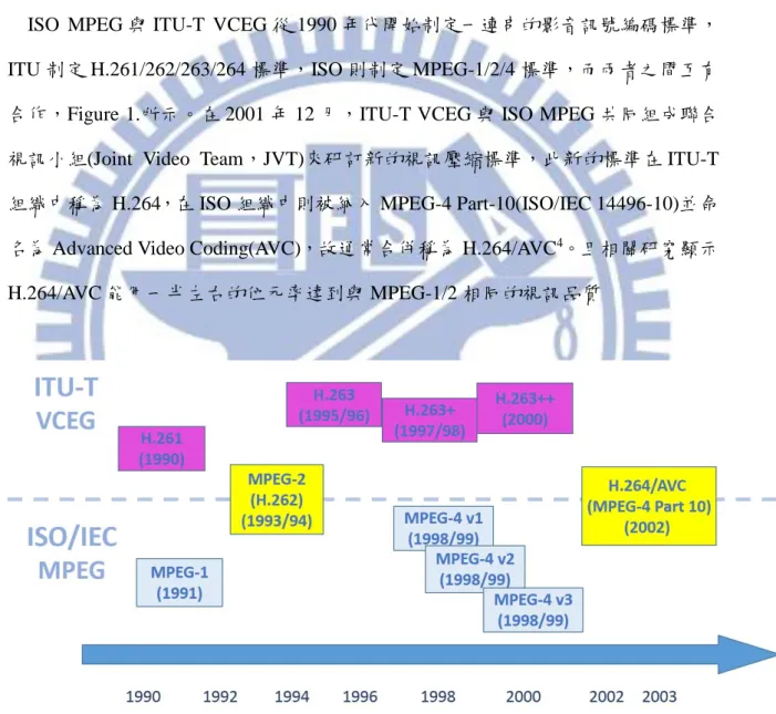
ISO MPEG 與 ITU-T VCEG 從 1990 年代開始制定一連串的影音訊號編碼標準, ITU 制定 H.261/262/263/264 標準,ISO 則制定 MPEG-1/2/4 標準,而兩者之間互有 合作,Figure 1.所示。在 2001 年 12 月,ITU-T VCEG 與 ISO MPEG 共同組成聯合 視訊小組(Joint Video Team,JVT)來研訂新的視訊壓縮標準,此新的標準在 ITU-T 組織中稱為 H.264,在 ISO 組織中則被納入 MPEG-4 Part-10(ISO/IEC 14496-10)並命
名為 Advanced Video Coding(AVC),故通常合併稱為 H.264/AVC4。且相關研究顯示
H.264/AVC 能用一半左右的位元率達到與 MPEG-1/2 相同的視訊品質
Figure 1. Chronological Table of Video Coding Standards
4
H.264/AVC 標 準 在 架構 上 包 含了 VCL(Video Coding Layer) 與 NAL(Natwork Abstraction Layer)兩層,VCL 為視訊壓縮的部分,其技術核心包含動作估計(Motion Estimation)、線性轉換編碼(Linear transform coding)、預測編碼(Prediction coding)、 去區塊效應濾波器(In-loop filter)、及熵編碼(Entropy)等技術,詳細內容會在後續小 節說明,NAL 提供 VCL 編碼資料與實際網路之間的介面,進行編碼資料的格式化, 加入必要的檔頭資訊(NAL header),在封裝成適當的傳輸單元,而 H.264/AVC 的 NAL 提供多種封裝方式,以方便適用於各種的通訊傳輸協定,如 Figure 2.所示,而 Transport Protocol 不屬於 H.264/AVC 標準的規範。
VCL (Video Coding Layer)
NAL
(Network Abstraction Layer)
視訊壓縮
格式化與封裝 編碼資料
H.264/AVC規格 定義範圍
RTP/IP TCP/IP MPEG-2
Systems 其他 NAL unit Transport Layer 傳輸網路 資料流 Internet Figure 2. H.264/AVC 分層圖
2.1.1 Profile
H.264/AVC 根據使用的編碼工作種類來提供十幾種 Profiles, 其中較常使用在消費 性電子產品的幾種 profiles 包括了 Baseline profile、Main profile、extension profile、High profile,不同 profile 規範了適合不同應用的編碼工具,前三種 profiles 的工具如 Figure 3 所示,至於 High profile 則是在 Main profiles 之上增加了 88 transform 等工 具。而相對應的影片解析度與位元率等資訊由不同的 Level 所規範。Baseline profile5
主要是應用在低複雜度,低延時的應用,所以適合應用在手持式裝置的多媒體支援, 本篇論文則是使用 H.264/AVC Baseline profile decoder 作為 reference design,Main profileadd 則增加了 coding tools(如 B slice 、CABAC ),故具有較好的壓縮效率,適 合應用於 HDTV 數位電視廣播,Extensio profile 則有高抗錯性的編碼工具(error resilient tools),以及增加 SP 和 SI slice,故適合於 streaming media application。
Baseline profile I slices P slices CAVAC Slice Grops And ASO Redundant Slice B slices Weighted Prediction Interlace CABAC SP and SI slices Data Partitioning Main profile Extended profile Figure 3. H.264 Profile
2.1.2 H.264/AVC 影像格式階層架構
H.264/AVC 的階層架構由小到大依序是 Sub-block、block、Macroblock(MB)、slice、 slice group、frame/field-picture、sequence,以 Baseline profile 常用的 420 取樣的 MB 而言,是由 16x16 點的 Luma(Y)與相對應的 2 個 8x8 點 Chroma(Cb 和 Cr)所組成, MB 可在分割成多個 16x8、8x16、8x8、4x8、8x4、4x4 格式的 sub-blocks,MB 為 H.264/AVC 解碼的最小基本單位,則所謂的 slice 是許多連續的 MB 的集合,如圖 Figure 4.所示,slice 為 H.264/AVC 格式中的最小可解碼單位(self-docedable unit),即 一個 slice 單靠本身的壓縮資料就能做解碼,不需要仰賴其他的 slice,而 slice 主要 可以分成三種,第一種為 I-slice, slice 的全部 MB 都採用 intra prediction 的方式編 碼;第二種為 P-slice,slice 中的 MB 使用 intra prediction 和 inter prediction 的方式6
來編碼,但每一個 inter prediction MB 最多只能使用一個移動向量(Motion vector);
第三種為 B-slice5,與 P-slice 類似,但是可以使用兩個移動向量,而本論文研究是
使用 baseline profile,所以不討論 B-slice 的情況。而 H.264/AVC 另外有增加兩種特 殊的 slice 類型(使用在 extension profie),第一種為 SP-slice(Switching P slice),為 P-slice 的一種特殊類型,可以用來串接兩個不同 bitrate 的 bitstream;第二種為 SI-slice(Switching I slice),為 I-slice 的一種特殊類型,除了用來串接兩個不同內容 的 bitstream 外,也可用來執行隨機存取(random access)。Slice group 由一個以上的 slice 所組成,在本論文沒有使用這個格式。Figure 5.為 H.264 Syntax。
I P P I
P P
Video frame Slice Macroblock I : Intra coding
P : Inter coding
Time Macroblock
Each MB is composed of 16x16 pixels
Figure 4. H.264/AVC Slice and MB
Figure 5. H.264 syntax
5 B 是指 Bi-prediction,與 MPEG-2/4 B-frame 的 Bi-directional 概念不同,H.264/AVC 不拘限於指定
7
2.2 H.264/AVC 核心技術
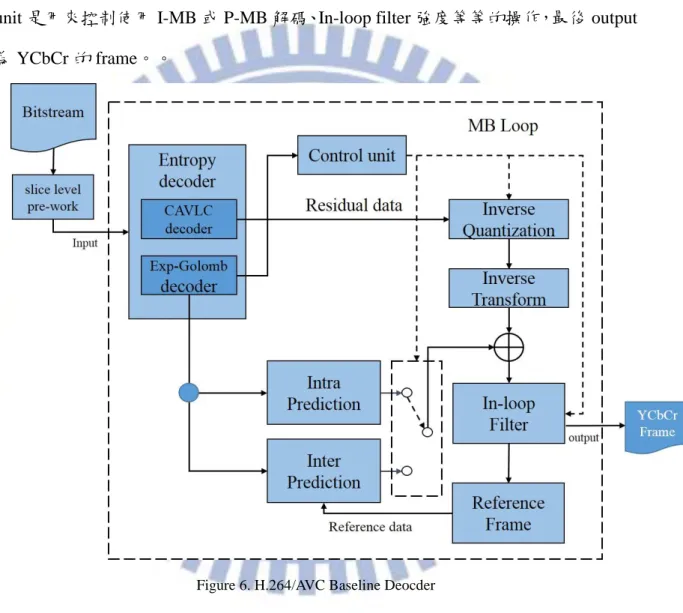
從 H.261 至今的主要的視訊壓縮標準都是遵循 Block-Based Hybrid Video Coding 的架構,如 Figure 6.所示為 H.264/AVC Baseline Deocder,而圖中(虛線內)在各個模
組執行的基本單位為 Macroblock(MB),接下來小節將對主要的模組做介紹6,Control
unit 是用來控制使用 I-MB 或 P-MB 解碼、In-loop filter 強度等等的操作,最後 output 為 YCbCr 的 frame。。
Figure 6. H.264/AVC Baseline Deocder
8
2.3 熵編碼(Entropy)
此模組是針對量化後的轉換系數和其餘的 H.264/AVC syntax 進行編碼,其目的是 去除編碼冗餘(coding redundancy)來提高壓縮比,而編碼冗餘是指量化後符號機率 並非完全相等,且符號之間也存在著相關性。 (1) Exp-Golomb在 H .264/AVC syntax 的部分指的是 Header information 或是 Motion Vector Difference、Prediction mode 等等的有關影像資訊,而這些資訊是使用 universal VLC(UVLC)中的名為 Exp-Golomb 編解碼技術,該技術是以採表的方式來完成,如 圖 Figure 7.,因此需要額外的記憶體來儲存編碼表。
9
(2) Contex Adaptive Variable Length Coding (CAVLC)
在轉換系數編碼的部分,H.264/AVC 提供兩套編碼技術,Contex-adaptive binary arithmetic coding(CABAC) 和 Contex-adaptive variable length coding(CAVLC) , CABAC 提供了較佳的壓縮效率,但相對的複雜度是高於 CAVLC,而在 baseline profile 是採用 CAVLC。
由於每個影像區塊在經過 Linear Transform 後會將大部分的能量集中在低頻的部 分,而在經由量化後會產生大量的為零係數,而末端的非零係數通常都是為正負
一,所以 CAVLC 是針對此特色來進行處理,先用 zig-zag oreder 的掃描方式7,如
Figure 8.所示,然後在將 4x4 區塊係數整理成一連串的係數,針對非零係數與為零 係數間位置的關係採用 run-level 的技術來做編碼。解碼則是利用 coeff_token 得知 非零數值與 TrailingOne 的個數,根據 TrailingOne 的個數可得知最後幾個的值為+1 或-1,其實不是 TrailingOne 的 Residual 則是按照其他方向由後到前依序解碼,根據 TotalZero 與 RunBefore,計算出每個非零數值與其前ㄧ個非零數值之間其零的個 數,並將這些零放入。
Figure 8. Zig-Zag order scan
7 把資料由 2D 轉向 1D 或反之
10
2.4 Inverse Transform and Inverse Quantization
H.264/AVC 轉換(Transform)的部分是採用類似 DCT(DCT-like)進行訊號能量集 中,與傳統 DCT,即 Figure 10.,差異是採的是純整數空間的轉換,在解碼端得到 的結果和編碼端相同,即不會產生 Mis-match 的情況,而且 H.264/AVC 在轉換時採
較小的 4x4 區塊運算8,可使用較短的運算元長度(16-bit)並只需要使用加法與乘法,
故降低在轉換上的複雜度,而小區塊的運算也能降低區塊效應(Blocking effect)的影 響,其 4x4 inverse transform 的轉換公式如 Figure 9.。
Figure 9. Transform formulas
Figure 10. DCT formulas
8 彩度(chroma)是採用 2x2 的矩陣轉換
11
H.264/AVC 提供量化器(Quantizer)來縮減轉換參數和降低編碼資訊,其原因是人 類視覺對於高頻影像部分敏感度較低,故可以做到降低編碼資訊而人眼感受不大。 而 H.264/AVC 提供 52 個量化步階(step sizes)可供選擇,其對應的量化步階(step sizes) 依指數非線性成長,相鄰的量化步階約差 12%,每隔六個量化步階其值變成原來的 兩倍,這樣的設計讓 H.264/AVC 可以適用於不同壓縮率的環境,其完整流程如 Figure 11.所示。
12
2.5 Intra Prediction
H.264/AVC 利用一張畫面內相鄰的 MB 的關聯性來減少原本大量的資料量,即拿 相鄰資料來預測(Prediction),而稱做 Intra prediction,而 Intra prediction 提供兩種不 同 block size 選擇,即 Intra 4x4 mode 和 Intra 16x16 mode。
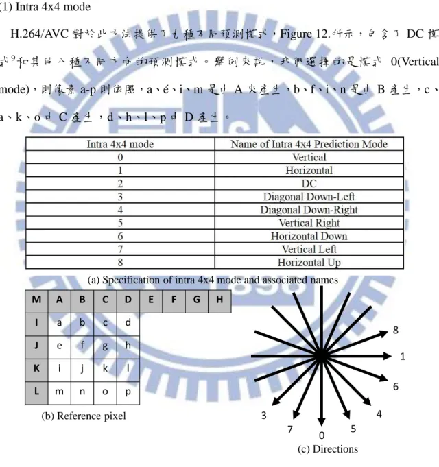
(1) Intra 4x4 mode
H.264/AVC 對於此方法提供了九種不同預測模式,Figure 12.所示,包含了 DC 模
式9和其他八種不同方向的預測模式。舉例來說,我們選擇的是模式 0(Vertical
mode),則像素 a-p 則依照,a、é、i、m 是由 A 來產生,b、f、i、n 是由 B 產生,c、 a、k、o 由 C 產生,d、h、l、p 由 D 產生。 M A B C D E F G H I a b c d J e f g h K i j k l L m n o p 0 1 3 7 5 4 6 8 (b) Reference pixel (c) Directions
(a) Specification of intra 4x4 mode and associated names
Figure 12. Intra 4x4 modes and their directions
13
(2) Intra 16x16 mode
H.264/AVC 則對於 16x16 亮度(luma)區塊提供四種不同的預測模式10,如 Figure
13.所示,在處理方式上 Intra 4x4 與 Intra16x16 是差不多的,由相鄰的 A-P 像素來 當作 a-p 之預測值,而如果有鄰近的參考區塊無法取得時(如畫面邊緣),則某些模 式則無法採用。 0 3 3 1 A B C D E F G H I a b c d a b c d J e f g h e f g h K i j k l i j k l L m n o p m n o p M a b c d a b c d N e f g h e f g h O i j k l i j k l P m n o p m n o p
(a) Specification of intra 16x16 mode and associated names
(b) Reference pixel (c) Directions
Figure 13. Intra 16x16 modes and their directions
14
2.6 Inter Prediction
動態影像(video sequence)是由連續的畫面(frame)所構成,每張畫面是景物(Object Scene)加上背景(Back Scene)所構成,在連續的畫面之間移動量較小時,背景通常不 變或相似度極高,景物通常則是以有規律性的方向移動,綜合以上以上景物與背景 的現象,在連續的畫面中畫面與畫面之間的關聯性很高,如 Figure 14 所示,因此 在畫面與畫面間進行預測編碼,我們稱之為 Inter Prediction11。在 H.264/AVC 視訊壓縮標準中提供了七種不同的 Macroblock partition 模式,有 P16x16、P16x8、P8x16、P8x8、P4x8、P8x4、P4x4,且每個 Macrblock 內部又可以 切成多個 sub-macroblock,有 8x8、8x4、4x8、4x4 形式,Figure 15.所示
Figure 14. Sample sequence
0 0 1 1 0 0 1 2 3 0 0 1 1 0 0 1 2 3 16x16 16x8 8x16 8x8 8x8 8x4 4x8 4x4
Figure 15. Partition of macroblock and sub-block
15
Inter Prediction 解碼的過程主要分成兩個部分,第一個部分為取得 Reference Index 和 Motion Vector(MV)資料,Reference Index 代表目前我們要解碼的 MB 參考到哪張 frame,這資料能從 Bitstream 中取得(由 Entropy 解碼),另外 MV 是代表目前解碼的 MB 和參考的 MB 之間的移動向量,而 H.264/AVC 為了減少 bitstream 大小,所以 沒有把 MV 直接紀錄在 Bitstream 中,只會紀錄 Motion vector differences(MBD),而
我們要算出 Motion Vector Predictor(MVP)在加上 MVD 才能取得 MV12,而我們把第
一個步驟稱為 Motion Vector Reconstruction(MVR)。
第二部分,當我們知道 Reference Index 和 Motion Vector 兩項資料後,先從 Reference Index 找出參考的 Frame,再利用 Motion Vector 取得 Inter Prediction Block,如 Figure 16.所示,接下來把經過 IQIT 後的 Residual Block 和 Inter Prediction Block 做重建(Reconstruct)動作,這動作我們稱為 MB Video Reconstruction(VR),而 以上兩個步驟就是 Inter Prediction 解碼的流程。
Figure 16. Inter Prediction13
12 計算方式為 MV = MVP+MVD
16
2.6.1 Sub-pixel interpolation
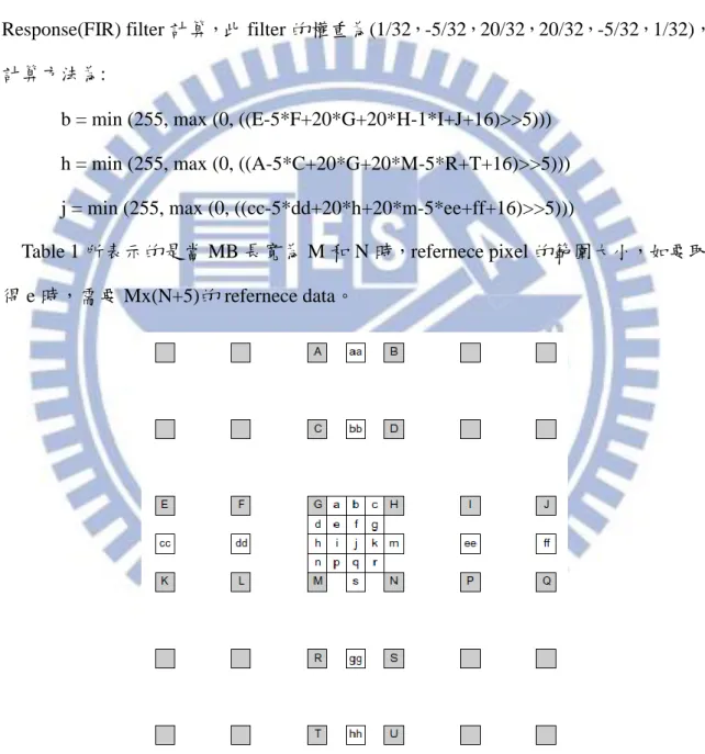
Sub-pixel positions sample 是不存在在 reference picture,所以需要使用 interpolation filter 使用附近的 image pixels 來建立 Sub-pixel,如 Figure 17 所示,灰色區塊為 full-pixel,白色區塊則是 sub-pixel,sub-pixel sample 需要使用 6 tap Finite Impulse Response(FIR) filter 計算,此 filter 的權重為(1/32,-5/32,20/32,20/32,-5/32,1/32), 計算方法為:
b = min (255, max (0, ((E-5*F+20*G+20*H-1*I+J+16)>>5))) h = min (255, max (0, ((A-5*C+20*G+20*M-5*R+T+16)>>5))) j = min (255, max (0, ((cc-5*dd+20*h+20*m-5*ee+ff+16)>>5)))
Table 1 所表示的是當 MB 長寬為 M 和 N 時,refernece pixel 的範圍大小,如要取 得 e 時,需要 Mx(N+5)的 refernece data。
Figure 17. Full-pixel samples (shaded blocks with upper-case letters) and sub-pixel sample positions (un-shaded blocks with lower-case letters) fro quarter-pixel sample luma interpolation
17
Table 1. The interplation filters and reference data size of one MxN luma partition of single direction
Interpolation position Interpolation filters Minimized reference data size
G No MxN
a,b,c 6-tap horizontal Mx(N+5)
d,h,n 6-tap vertical (M+5)xN
e,f,g,i,j,k,p,q,r 6x6 tap filter (M+5)x(N+5)
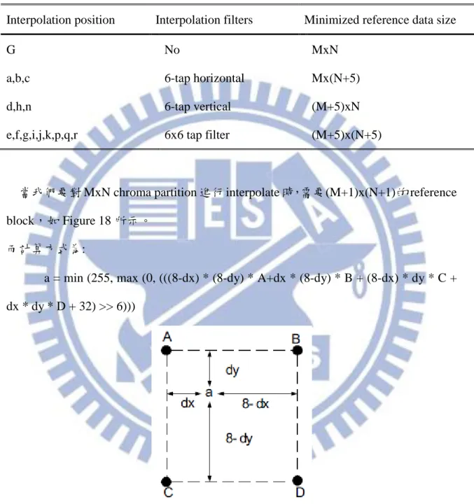
當我們要對 MxN chroma partition 進行 interpolate 時,需要(M+1)x(N+1)的 reference block,如 Figure 18 所示。
而計算方式為:
a = min (255, max (0, (((8-dx) * (8-dy) * A+dx * (8-dy) * B + (8-dx) * dy * C + dx * dy * D + 32) >> 6)))
Figure 18. Sub-pixel sample position a in chroma interpolation and surrounding full-pixel position samples A, B, C, and D
18
2.7 In-loop Filter
H.264/AVC 是以區塊為單位進行處理,所以會有區塊效應(Blocking effect),因此 我們需要 In-loop filter 來消除區塊效應,來改善影像品質。
在 In-loop Filter 的流程中,由兩個主要的參數來控制 Filter,第一個為 Boundary Strength(BS),是用來決定該使用何種強度的濾波器(Filter)來執行濾波的動作,而 BS 由 Figure 19.公式來決定。另一個重要參數為 Threshold(α、β、indexA),而此
參數是用來判斷是否為 true edge14,而 In-loop filter 流程如 Figure 20.所示。
Figure 19. Determining the boundary strength
p3 p2 p1 p0 q0 q1 q2 q3 p1 p2 q0 q1 q2
Get BS Get Threshold
Input Luma Pixels Input Chroma Pixels Boundary strength
Coding Information QP
Edge Filter ( Deblocking filter )
p1 p2 q0 q1 q2 p3 p2 p1 p0 q0 q1 q2 q3
Filtered Pixels
Figure 20. In-loop filter 流程圖
19
2.8 Google Android’s H.264/AVC baseline decoder
在我們的研究中,single-core H.264/AVC decoder 是從 Google Android project[20] 取出來的 baseline reference decoder,此程式碼位於 Figure 21 所示 Libraries 中的 Media Framework 部分,Figure 22.為 OpenCore 的架構,H.264/AVC 為 Video Codecs 其中之ㄧ。
Figure 21. Android System Architecture
20
三、Introduction to Parallel H.264 Decoding Scheme
此章節是分析 H.264 Baseline Decoder 平行化的方式,首先 3.1 節為 Related work 來探討 Parallel H.264 Decoder 的發展與技術,第 3.2 節就 H.264/AVC 架構上與資料 結構上的相依性做討論。因為本論文是探討軟體平行解碼,而目前在傳統 Symmetric Multi-Processor(SMP)架構下的軟體平行解碼大多採用 Data-Level Parallelism(DLP) 的技術,因此接下來在 3.3 節針對 DLP Video decoder 與其實作進行詳細討論。在下 一章,我們會探討針對特殊架構處理器設計 Task-Level Parallelism(TLP)的視訊平行 解碼器進行討論。
3.1 Related Work
現今主要的視訊壓縮標準大多只有支援 slice-level coarse-granularity 的 DLP 平行
計算15,如果想採用 MB-level 的 fine granularity DLP 運算,在視訊格式中存在著資
料相依性(Data dependencies),而相關的平行演算法使用不同級別的劃分方式來確保 沒有資料相依性的問題。在 frame level partitioning 是不適用於嵌入式系統中,因為 其 inter prediction [1] 和 buffer size 的限制,尤其是在高解析度的視訊(如 FHD 或 HD),其記憶體需求會是ㄧ個極大的負擔。而在 slice level partitioning,除了 MPEG-2 標準能充分的發揮平行化,其他主流的標準,如 MPEG-4、H.264/AVC 皆無法在此 級別發揮良好的平行化,因為 MPEG-2 標準定義每個 MB row 為一個獨立的 slice, 而在 H.264/AVC 可以允許一個 frame 只有一個 slice,而大多視訊壓縮也皆採用此壓
縮方式16,因此最適合的級別將會是 MB level partitioning,但 MB level 仍有資料相
依性的問題需要解決,將會在之後章節介紹。雖然 slice level partition 在實務上平行 度有限,但在實作上,因為每個 slice 為獨立解碼的基本單位,所以在平行化的實
15 最新的 HEVC 標準提供 fine-granularity DLP 平行化計算的支援,如 Wavefront 與 Titles 技術但會
犧牲 coding efficiency。
21
作上負擔不大,而 FFmpeg H.264 decoder[21]就有提供 slice-level parallelism 的支援。 使用 MB level 的平行化方式主要分成兩類,Data level parallelism(DLP)和 Task
level parallelism(TLP)兩種,DLP 是讓不同的 threads 或 cores 同時去執行相同的
function 但不同範圍的 input data,Van Der Tol et al.在 [2] 提出 Stairway-shaped data
partition,用來減少 inter-partition 的相依性。Seitner et al.在 [3] 中,分析了多種不 同 partition 方式,如 single row(即每個 thread 或 process 對 single row 作解碼動作)、 Multi-column partition 等等,探討其 cache performace、buffer size、data transfer for
reference data 在不同 partition 的情況。而在 [4] [5] [6] 中,在探討 DLP 之 scalability, 並提出 2D-Wave 方式,且更進一步的加入 frame level 的平行化,稱之 3D-Wave, 而此種方法可以大幅提升 MB 平行化的程度,但存在了一些限制,如需限制 encoder 端的 MV range 和 reference list number,且在核心數和記憶體有限的嵌入式系統中,
效益並不顯著。而也有相關研究在 Cell Broadband Engine17上做分析 [7] [8],利用
其多個 Synergistic Processing Units(SPUs),來同時執行不同的 MB,但其平台在撰 寫 Parallel programming 其 Local storage 和 Shared memory 資料之間的管理,對於 Programmer 是ㄧ個負擔。Jike Chong et al. 在 [9] 針對 data scheduling 的挑戰 (即平 行度與複雜度等等) 與技術進行討論。
TLP 為分別讓指定的 thread 或 core 去執行不同的 function(或稱 task),或以 pipeline 的方式稱之。Schöffmann et al.在 [10] 提出了 static partition pipelining,分成五個
17 為 IBM 和 SONY 共同開發之平台
22
stage,而此方法會存在 load balance 的問題,且在 thread 個數大於核心數的情況下, 平行化效能會因為 thread scheduling 的影響,而造成加速幅度有限。Minsoo Kim et al. 在 [11] 提出 Dynamic load balancing method 在其雙核心 DSP 平台,系統架構包含 了雙核心 DSP、VLD 硬體、MC 硬體、Deblocking 硬體和 SDRAM,因此在整個解 碼流程中,DSP 只負責少許的部分,而 Minsoo Kim et al 在 [12] 擴充其系統架構 至四核心的 DSP,且 Debloking 和 MC 也由 DSP 處理,另外提出了減輕 system bus 頻寬的平行化技巧。Chen, Ding-Yun, et al 在 [13] 在雙核心平台提出藉由監控兩核 心之間 buffer 來動態更改其 partition 來解決 load balance 問題。Chun-Jen Tsai et al. 在 [14] 提 出 Application Processor Architecture for Multi-Core Software Video Decoding,並利用提出的 Inter-preocssor communication (IPC) controller 能使得 TLP
deocder 減輕 system bus 頻寬,以及減少資料傳輸所造成的開銷。
3.2 Macroblock dependencies of H.264/AVC
H.264/AVC 在 Macroblock level 的資料相依性可以分成三類,如 Figure 23.和 Figure
24.所示。Figure 23 (a) Intra prediction 是利用目前解碼的 Macroblock 其左邊、左上、 上方、右上之 pixels 來作為 prediction 之依據,而此部分的解碼能利用放在同一顆 核心來執行,可以減少用來解決相依性的 inter-preocessor communication。Figure 23 (b) Deblocking filter 部分則是需要上面 MB 的最後四個 rows 和左邊 MB 的最後四 個 columns 的 pixels 值,用來解決 blocking effect,另外還需要目前 MB 其上面與左 邊 MB 的 Motion Vector 和 Reference Index 來計算 Boundary Strength(BS)。最後 Figure
23
23 (c) Inter-prediction 則是需要確保目前 frame 所要參考的 frame 其位置(MB or
Sub-MB)已經解碼完畢,Meenderinck et al.在 [4] 中,有利用在 H.264/AVC encoder
端限制 SearchRange 和 NumberReferenceFrames18來增加 Scalability。
另外 Entropy 解碼部分因為現今視訊標準採用的壓縮編碼法(如 VLC,AC)再兩個
synchronization points 之間必須進行完全循序的資料處理。而且不少 video bitstreams 每張影像只插入一個 synchronization point,因此此模組不會加入至平行化的實作 中,意思是先執行完 Entropy 在進行之後模組的平行化,因此不討論 Entropy 模組 的資料相依性。 Frame n-1 Frame n (a) Intra-prediction dependency (b) Deblocking filter dependency (c) Inter-prediction dependency Figure 23. Dependencies of H.264/AVC
Intra pred. MV pred. Intra Pred. MV pred. loop filter Intra pred. MV pred. Intra pred. MV pred. Loop filter Current MB
Intra pred. : pixel prediction for the current MB requires data from this block.
MV pred. : motion vector prediction for the current MB requires data from this block. Loop filter : de-blocking of the current MB requires
data from this block
Figure 24. Data dependency neighborhood of the MB decoding process
24
3.3 Data-level Parallelism
在 3.3.1 節會簡單的介紹 DLP 並介紹使用何種 scheduling,第 3.3.2 節會介紹本論 文實作的 static scheduling,而第 3.3.3 則是對 DLP 的總結。
3.3.1 DLP Overview
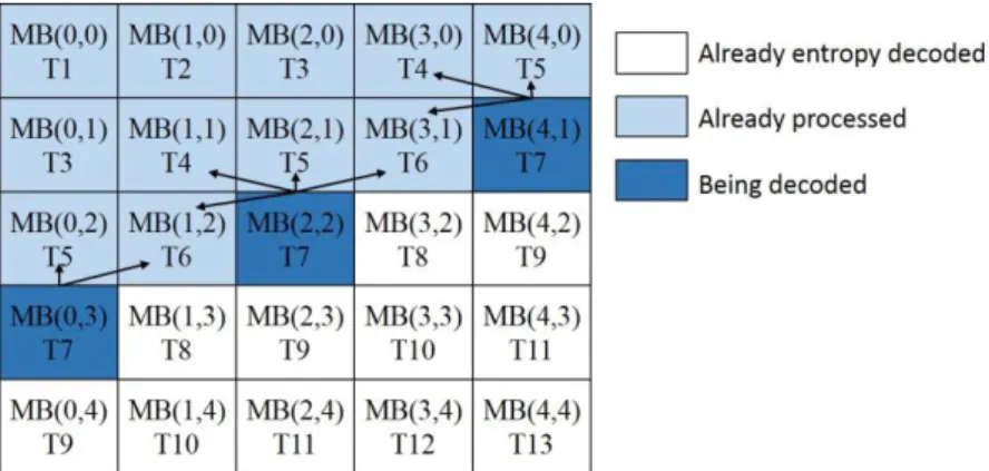
Data-level Parallelism(DLP) decoder 又可以稱做 Wavefront-based decoder,DLP 是 讓不同的 threads 或 cores 同時去執行相同的 function 但不同範圍的 input data,如 Figure 25.所示。根據 4.2 節可以知道 H.264/AVC 在結構上存在的相依性,而依照其 相依性在 MB level 的平行化,我們可以很容易的推出 Figure 26.19,此圖為一個 5x5 的 frame,其代表的是當 T1 時間點時只存在一個 MB(0,0)被解碼,而當 T7 時間點 時,則可以三個 MB(4,1)、(2,2)、(0,3)同時被解碼,以此類推,當解析度放大至 Full High Definition(FHD,1920x1080)時,在整個解碼過程中平均約有三十個 MB 能同 時進行解碼,甚至最多能達到同時有六十個 MB 能並行解碼,如 Table 2.所示(Slots 代表達到最高 MBs 時 times slots 個數)。 Proc. 1 Proc. 2 Proc. 3 Proc. 4 Video frame
Figure 25. Data-level Parallelism
25
Figure 26. Exploiting MB parallelism in the spatial domain.
DLP 在 MB-level 擁有許多優點,最明顯的就是增加 scalaility(參考 Figure 26.)。 而 Á lvarez Mesa 在[5] 計算 Maximum speedup 和最高處理器的使用數都能證實 DLP 的高擴展性。另外就是在 dynamic scheduling 中能做到較好的 load balance,因為對 每一個 MB 解碼時間不固定,而是要取決於 MB 的形態(I 4x4 or I 16x16 or P 8x8 etc.) 與資料量(如 residual data)。但本論文是採用 Static scheduling,即指定某範圍的資料 (MB)給指定的 Thread 或 Core 解碼,其原因是本研究是以嵌入式手持式平台(如 smart phone)為目標,使用 dynamic scheduling 需要維護 FIFO queue(用來讓 worker thread 取資料來解碼),且 dynamic scheduling 複雜度會相對於 static scheduling 高,而在手 持式裝置上處理器核心數有限的情況,無法從 scalability 得到好處,因此本論文採 用是 static scheduling,可以減少額外的記憶體使用,也能減輕 scheduler 的負擔。
Table 2. Maximum parallel MBs for several resolutions using DLP
Resolution MBs Slots QCIF 176x144 6 4 CIF 352x288 11 8 SD 720x576 23 14 HD 1280x720 40 6 FHD 1920x1080 60 9
26
3.3.2 Static scheduling 實作與技術
首先先把 H.264/AVC decoder 分成兩部分,第一部份為 Main thread,是用來執行 Entropy 跟 Scheduling,第二部分則是 worker threads,是執行 IQIT、MC、Intra 或 Inter prediction 和 Loop filter,如 Figure 27.所示。由 Main thread 執行 Entropy 的原 因是在 Entropy 模組中需要以 Raster scan 的順序進行解碼,且往後模組需要的資訊 皆要在 Entropy 模組中取得,所以 Entropy 這部分無法加入到平行化的部分且要先 被完成,而這也是 DLP 缺點之ㄧ。
論文中 DLP 的 Data partition(splitting strategy)是採用 Single-row approach,如 Figure 28.(圖上之數字代表 Processors 編號)、Figure 29.所示,即每個單一行上的 MBs 由一個 Processor 解碼,更正式的說法為,我們假設 N 為 Processors 個數,當 y mod N = i 時,Processor i ∈ {0,…,N - 1} 其解碼資料對映到 y th 行 MBs 上。 Bit Stream Parsing CAVLC (UVLC Inverse Quantization Linear Transform Motion Compensation Intra or Inter Prediction Reference Frame store Loop Filter (Deblocking) Input Output Entropy Main thread
(Scheduler) Worker threads
Figure 27. DLP- Flow chart
27 Thread 4 waiting Thread 4 Thread 4 (a) (t = N ) (b) (t = N +1) (c) (t = N+2 ) Being decoded
Already entropy decoded
Already processed
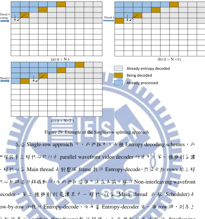
Figure 29. Example of the Single-row splitting approach
在這 Single-row approach 下,我們採用了兩種 Entropy decoding schemes,我
們預設有三顆核心可以由 parallel wavefront video decoder 所使用,第一種機制為讓 一顆核心為 Main thread 去對整張 frame 執行 Entropy-decode,然後分配 rows 給三顆 核心同時進行解碼動作,而我們把這個方法在本論文稱作 Non-interleaving wavefront decoder 。 第 二 種 機 制 則 是 讓 其 中 一 顆 核 心 ( 為 Main thread 或 稱 Scheduler) 去 row-by-row 的執行 Entropy-decode,而每當 Entropy-decoder 完一個 row 時,則馬上 分 配 給 其 他 worker thread(core) 執 行 解 碼 , 而 我 們 把 此 方 法 稱 作 Interleaving wavefront decoder,此方法可以解決 Static scheduling 所造成的 Main(或稱 Master) thread 大部分時間都是在等待其他 worker threads 完成解碼,因此可以讓整體效能提 升。
28
(a) Non-interleaving wavefront decoder
Main Thread
Slice Start Entropy One Frame
Slice End? Slice Finish Yes No Notify Thread n Row Data Ready
Thread1 Row start Thread2 Row start ThreadN Row start ‧ ‧ ‧
Check Check Check
Enable Dec. MB Filter MB Row End? No Yes Enable Dec. MB Filter MB Row End? No Yes Enable Dec. MB Filter MB Row End? No Yes
Thread Start Thread Start Thread Start
Wait for new row Wait for new row Wait for new row Wait for thread
corresponds to the row
Scheduler Worker Worker Worker
(b) Interleaving wavefront decoder
Main Thread
Slice Start Entropy One Row
Slice End? Slice Finish Yes No Notify Thread n Row Data Ready
Thread1 Row start Thread2 Row start ThreadN Row start ‧ ‧ ‧
Check Check Check
Enable Dec. MB Filter MB Row End? No Yes Enable Dec. MB Filter MB Row End? No Yes Enable Dec. MB Filter MB Row End? No Yes
Thread Start Thread Start Thread Start
Wait for new row Wait for new row Wait for new row Wait for thread
corresponds to the row
Scheduler Worker Worker Worker
Figure 30. Two different entropy decoding schemes
流程如 Figure 30.所示,而圖中 Wait for new row 階段是利用 Hardware Mutex 來維
護,建立 row 個數的 Mutex20並使其狀況為 lock,每當一個 row 執行完 Entropy-decode
時,Scheduler 呼叫 unlockMutex(row_num)動作,這時候 worker thread 就能順利對 該 row 進行解碼。而 Check 階段則是進行 checkNeighborMB 的動作,當 MB 要進
29
行解碼時,要確保其附近的 MBs 是已經解碼完(原因可看 4.2 節),否則會進入 busy waiting 直到條件觸發,而這部分就是 DLP 的瓶頸所在,假如把 flags 放置在 DDR2,
則需要不斷的呼叫 cache invalidation function21,造成效能的下降,因此在 DLP 設計
中的 flags 都放置在 On-chip shared SRAM(uncached memory),但當多顆處理器頻繁 的讀取 flags,會導致整體效能受影響。
另外 DLP 在資料結構上的設計,主要分為三種 slice-level data structure 與 MB-level data structure 與 Intra prediction 所需要的資料,slice-level 主要是儲存一張 slice 中共 用之資料(如 slice_id、slice type、PicWidthInMbs),所佔之空間為 552 bytes,而 MB-level(如 mvL0、ref_idx_L0、mbMode、CBP)則總共為 2KB,假設影像解析度為
CIF(352x288),則 Intra prediction 所需要的資料量為 1056 bytes22,因此當對一張 slice
進行解碼時,需要 794 KB23資料儲存在 DDR2(shared memory),假如在進一步把解
析度放大至 VGA(640x480),約需要 2.4MB 的資料量,有此可知,DLP 對於記憶體 的需求其實是不容忽視的,尤其是在高解析度的視訊上。
21 本論文中使用的 cache 為 Non-coherent cache 22 2 x (PicWidthInMbs<<4) x 3/2 = 1056 bytes
30
四、Proposed Parallel H.264 Decoder Scheme
本論文所採用的是在特殊架構下的 task-level parallel video decoder,系統架構如 Figure 31 所示,架構的設計細節請參考[14]。在第 4.1 節會先簡介 Task-Level Parallelism(TLP)的 H.264 解碼器。第 4.2 節則是會介紹本論文中的三種 TLP 實作與 其技術,即 static pipeline partitioning、Dynamic pipeline partitioning using Macroblock mode 和 Dynamic pipeline partitioning using monitoring buffer,而第 4.3 節則是對 TLP 平行解碼時記憶體的使用做一個討論。
L2 cache
L1-I L1-D L1-I L1-D L1-I L1-D L1-I L1-D
system bus DRAM memory controller DDR2/3 memory chips
Application Processor SoC
Other peripheral controllers
transceivers Coherent cache subsystem
I-BUS2 D-BUS2
IPC controller IPC controller IPC controller IPC controller 2-port Local Memory 2-port Local Memory 2-port Local Memory 2-port Local Memory RISC 0 RISC 1 I-BUS1 D-BUS1 I-BUS2 D-BUS2
I-BUS1 D-BUS1 I-BUS1 D-BUS1 I-BUS1 D-BUS1
RISC 2 RISC 3
I-BUS2 D-BUS2 I-BUS2 D-BUS2
Figure 31. Application processor 架構圖
4.1 TLP Overview
Task-level Parallelism Video Decoder 可以稱作 Pipeline-based Video Decoder,TLP 是讓每個 processor core 執行一個 stage,或稱執行 task,如 Figure 32.所示,而進行
31
解碼的基本單位為 16x16 Macroblock。TLP 設計上主要有兩個議題,即 scalability problem 和 load balancing problem,在 pipeline 的平行化中 scalability problem 主要是 受限於 pipeline stages 的個數,如 Figure 33.所示,H.264/AVC 在 pipeline 解碼時, 對單一 Marcoblock 的解碼程序分成七個步驟,即 Entropy Decoding(ED)、Intra Mode
Reconstruction(IMR) 或 Motion Vector Reconstruction(MVR) 、 Inverse
Quantization(IQ) 、 Inverse Transform(IT) 、 Intra Prediction(IP) 或 Motion Prediction(MP)、MB Video Reconstruction(VR)、In-loop Filter(ILF),但因為為了減少 inter-stage communication 負擔與達到較好的 load balancing,大部分的實作會把解碼 流程合併成三或四個 pipeline stages,但假如 inter-stage communication 負擔可以忽 略的情況,事實上可以在對目前七個步驟在做細分,切成為 fine-granularity stages, 使得更輕易達到 load balancing,例如 H.264/AVC 之中運算成本較高的 In-loop filter, Wang 在[15]提出在 Deblocking filter 上使用 wavefront-based 的平行化方式,而其切 割非相依性資料的方式可以利用在 MB-level pipelined 上,在 In-loop filter 實作上, 會先對 4x4 垂直邊(vertical edges)進行處理,再來對 4x4 平行邊(horizontal edges)做 處理,因此簡單的切割方式是垂直為一個 stage,處理平行邊也獨立一個 stage( 利
用[14]中討論 independent pixel),所以至少24能再獨立出兩個 stages,而在現今大部
分的手持式應用處理器不超過八顆 RISC 核心的情況下,scalability 不會是我們研究 上對 TLP 設計上的主要關注議題。
32 Video frame Proc. 1 Proc. 3 Proc. 2 Proc. 4 Task
Task Task Task Task
Task Task
Figure 32. Task-level Parallelism (a) I-MB decoding steps:
(b) P-MB decoding steps: Entropy Decoding (ED) Motion Vector Reconstruction (MVR) Inverse Quantization (IQ) Inverse Transform (IT) Motion Prediction (MP) In-loop Filter (ILF) Entropy Decoding (ED) Intra Mode Reconstruction (IMR) Inverse Quantization (IQ) Inverse Transform (IT) MB Video Reconstruction (VR) In-loop Filter (ILF) MB Video Reconstruction (VR) Intra Prediction (IP)
Figure 33. The decoding steps of an I-MB and a P-MB of H.264/AVC
Load balancing 主要是因為對每個 Macroblock 解碼是 variable complexity,造成有 些解碼時間是消耗在 synchronization 上面,而我們這部分使用每兩個 processor 之間 設置一個 FIFO circular buffer,用來吸收因為 variable complexity 所造成的時間消 耗,如 Figure 35.所示,我們使用了四顆核心,所以我們使用了三個 FIFO circular buffer,Input buffer 用來放置壓縮後視訊的 bitstream data,buffer #1 與 buffer #2 則 是放置 MB 解碼所需要的資訊,在我們的實作中,為了避免需要 pack 與 unpack 處 理,因此兩個 buffer 的資料結構是相同的,而每個 buffer node 資料量為 2KB,另外
33
除了 Input buffer 放置在 DDR2,其餘兩個 buffer 皆是放置在處理器的 local memory (為 on-chip memory),放置在 local memory 原因為軟體實作的 pipeline 不像硬體 pipeline 般,能將暫存資料(或 intermediate data)儲存在 on-chip pipeline registers,通 常是儲存在 memory bank(不管是 on-chip SRAM 或 off-chip DRAM),因此讀寫須透 過 system bus,而不幸的事是 system bus 可能會被其他 tasks 或 device controllers 使 用,而造成效能上的影響,因此把資料放置在 local memory 則可以減少對 system bus bandwidth 的使用。
4.2 TLP 實作與技術
Pipeline-based video decoder 的效能是非常仰賴於每個 pipeline stages 的平衡,因 為每個 Macroblock 解碼複雜度變化是非常明顯的,所以很難利用固定的 stage partition 來達到接近完美的 load balancing,因此我們才在每兩個 pipeline stages 之間 加入 FIFO circular buffer,來吸收因為 MBs 擁有不同解碼複雜度所造成的負擔,但 這樣還是無法接近完美,因此我們在提出了兩種 Dynamic pipeline partitioning 的方 法 , 所 以 接 下 來 章 節 會 就 (1)Static pipeline partitioning 、 (2)Dynamic pipeline partitioning using Macroblock mode 和 (3)Dynamic pipeline partitioning using monitoring buffer 三種實作來介紹。
34
1) Static pipeline partitioning
如 Figure 34.所示,每個核心執行固定的 tasks,Core 1 執行 ED、MVR 或 IMR25,
會這樣分配是因為 MVR 與 ED 會共享資料,特別是目前 MB 與鄰近 MBs 的 MV 和 refIdx,MV 與 refIdx 儲存在 DDR2,因此當這兩個 task 分配在不同的核心時,這兩 個核心會在 DDR2 讀取同樣的資料,故放在同核心就只要在 cache 中讀取,可以減 少 system bus 的使用。Core 2 則是執行 IQIT、MP 或 IP、VR,這部分是三個核心 中負載最重的一顆(因為受限於核心數),而 Core 3 則是單純執行 ILF。
我們知道 MB 的解碼時間與 coding modes 有相當大的關係,舉例來說,當目前解 碼的單位為 Skipped Macroblock 時,則在 ED 時會消耗很少的時間,而相對的,當 解碼單位為 Intra Macroblock 時,ED 需要花費較多的時間解碼,其原因為 Intra Macroblock 通常擁有較多的 Residual bits。Table 3.所示為在五個 MPEG 測試視訊, 為各種 Macroblock types 的分布與加速比,我們可以很輕易的注意到在 News 影像 中當 skip MB 比重增加時,則效能會下降,而當 inter MB 比重上升,效能則相對上 升。 Core 1 (ED + (MVR or IMR) ) Core 2 (IQ + IT + (MP or IP) + VR) MB2 data
. . .
MB3 data MB4 bits. . .
MB5 bits Core 3 (ILF) MB0 data. . .
MB1 data DDR2 memory NAL units Reference framesInput Buffer Dual-mode
buffer #1 Dual-mode buffer #2 Pipeline stage 1 Pipeline stage 2 Pipeline stage 3
Figure 34. Static pipeline partitioning for the P-MBs and I-MBs of H.264/AVC
35
Table 3. Macroblock mode distributions and performance (use static pipeline partitioning)
Sequence Bitrate Intra MB (%) Inter MB (%) Skip MB (%) Speedup ratio
Crew 512 k 14.4 62.8 22.8 2.54 1.5 m 15.4 76.5 8.1 2.63 Foreman 512 k 4.1 66.2 29.7 2.56 1.5 m 4.2 80.4 15.4 2.74 Mobile 512 k 0.5 73.1 26.4 2.47 1.5 m 0.5 86.4 13.1 2.72 News 512 k 1.4 29.2 69.4 2.31 1.5 m 1.8 46.4 51.8 2.74 Stefan 512 k 3.0 59.4 37.6 2.29 1.5 m 3.8 72.9 23.3 2.54
The percentages of the macroblock modes are computed for the whole sequence of 300 frames.
Skip MBs 影響效能的原因是很簡單的,當在視訊中一連串的 skip MBs 會造成 ED 解碼時花費很少的時間,而當 FIFO circular buffer #1 深度不足時,在短時間內,第一 顆核心就會因為 buffer 滿載而閒置,理想上,FIFO circular buffer 其大小是要越大越 好,但現實中會受限於 local scratchpad memory 的容量限制,而為了解決這個問題, 我們提出了 Dynamic pipeline partitioning。
2) Dynamic pipeline partitioning using Macroblock mode
Dynamic partition 是在 Execution time 來決定目前的 partition 方式,能依照目前解 碼情況來改變,這樣可以避免和 Static partition 般,因為一連串的 Skip MB 造成第一 顆 核 心 與 第二 顆 核 心 的 負 載量 不均 , 而我們 用 來判 斷動 態 切割 的 依 據是 利 用 macroblock type,當 macroblock type 為 skip MB 時,使用 Figure 35(a)方法,圖中 SNIP 為執行 SaveNeighborForIntraPred,其功能是儲存目前 MB 部分 pixels,作為 Intra prediction 的參考資料,而 SNIP 必須固定在同一顆核心處理,否則需要把其 SNIP 資 料儲存在 DDR2,會影響解碼效能。
36 (a) First mode
Core 1 ED+MVR+IQ +IT+MP+VR Core 2 SNIP MB2 data . . . MB3 data buffer #1 . . . MB4 bits MB5 bits Input Buffer MB0 data . . . MB1 data buffer #2 Core 3 ILF Core 1 ED+IMR Core 2 IQ+IT+IP+VR +SNIP MB2 data . . . MB3 data buffer #1 . . . MB4 bits MB5 bits Input Buffer MB0 data . . . MB1 data buffer #2 Core 3 ILF
(I) P-MB decoding steps
(II) I-MB decoding steps (b) Second mode Core 1 ED+MVR Core 2 IQ+IT+MP+V R+SNIP MB2 data . . . MB3 data buffer #1 . . . MB4 bits MB5 bits Input Buffer MB0 data . . . MB1 data buffer #2 Core 3 ILF Core 1 ED+IMR Core 2 IQ+IT+IP+VR +SNIP MB2 data . . . MB3 data buffer #1 . . . MB4 bits MB5 bits Input Buffer MB0 data . . . MB1 data buffer #2 Core 3 ILF
(I) P-MB decoding steps
(II) I-MB decoding steps
Figure 35. (a) ~ (b) Two kinds of different partition for dynamic pipeline partitioning using MB mode
為了讓 MB types 影響平行化效能能更容易被理解,如 Figure 36、Figure 37、Figure 38 和 Figure 39 所示,為兩種 software pipeline decoder(static 和 dynamic pipeline partitioning schemes)的加速比,而測試視訊為 Crew 1.5mbps 和 Stefan 512kbps,可 以很明顯的發現 bits 數下降的 frame 與 speedup ratio 是有對應的,bits per sample 與 skip MB 有很大的關係,更進一步的觀察 Figure 39,就能發現當 Skip MB 數上升(尖 峰),會對應到較低的 speedup ratio,而在 Crew1.5mbps 的部分,能觀察出 speedup ratio 的尖峰是對應在 bits per sample 的尖峰也是對應在 number of the intra 4x4 的尖峰。 而 Figure 37 所示,Stefan 512kbps 中 skip MB 比重較重,更精確的說法是,出現連 續的 skip MB 比重較高,因此能看到當我們採用 dynamic partition 時,效能有顯著 的改進,而在 skip MB 比重較低的 Crew 1.5mbps 影響就有限。
37 0 50 100 150 200 250 300 2 2.5 3 3.5 frame number sp e e d u p r a ti o dynamic static 0 50 100 150 200 250 300 0 5 10 15x 10 4 frame number b it s p e r sa m p le
Figure 36.Top: the speedup ratio of the dynamic (use MB type) 26and static pipeline partition decoder for
[email protected]. Bottom:bits per frame of the video sequence
0 50 100 150 200 250 300 1.5 2 2.5 3 frame number sp e e d u p r a ti o dynamic static 0 50 100 150 200 250 300 0 2 4 6 8x 10 4 frame number b it s p e r sa m p le
Figure 37. Top: the speedup ratios of the dynamic (use MB type) and static pipeline partition decoder for [email protected]:bits per frame of the video sequence
38 0 50 100 150 200 250 300 2 2.5 3 3.5 frame number sp e e d u p r a ti o 0 50 100 150 200 250 300 0 100 200 300 frame number n u m b e r o f 4 x 4 M B s dynamic static [email protected]
Figure 38. Top: the speedup ratio of the dynamic and static pipeline partition decoder for [email protected]. Bottom: the number of the I4x4 MBs
0 50 100 150 200 250 300 1.5 2 2.5 3 frame number sp e e d u p r a ti o 0 50 100 150 200 250 300 0 100 200 300 400 frame number n u m b e r o f S k ip M B s dynamic static Stefan@512k
Figure 39. Top: the speedup ratio of the dynamic and static pipeline partition decoder for Stefan@512kbps. Bottom: the number of the Skip MBs
39
在我們的 static pipeline partition decoder 設計中,總共有三個 statges,第一個處理 Entropy decoder 和 Intra mode 或 Motion Vector Reconstruction,第二個處理 IQ、IT、 MB prediction 和 Reconstruction,而第三個則是執行 In-loop filter,而在 decoder 中 有兩個 FIFO circular buffer,如 Figure 34 所示,每個 buffer node 具有相同的資料結 構,而 speedup ratio 是直接被 buffer 是否 underflow 或 overflow 影響,假如在解碼 的過程中 buffer 不存在 underflow 或 overflow,則平均 speedup ratio 將會接近於三 倍,但現實中每個 MB 為 variable complexity,因此可能會造成 underflow 或 overflow,而效能因此被受影響。Figure 40 為 Stefan@512kbps frame #1 在 runtime 時 buffer depth 增長情況,frame #1 為此 sampley 在 static partition pipeline decoder 中最低 speedup ratio(1.99)的 frame,可以發現第一個 FIFO 幾乎都處於 overflow 狀 態,第二個則是 underflow,而我們在使用 dynamic partition,就能發現第一個 buffer overflow 的情況舒緩了許多,效能也提升到 2.65 倍。Figure 41 為 [email protected] frame #152,是該 sample 的 speedup ratio 最低的 frame,一樣存在的同樣問題,雖 然 dynamic partition(skip mode)有改善,但 buffer ovderflow 情況依然明顯,因此換 個角度,從 FIFO buffer 這邊出 0 50 100 150 200 250 300 350 400 0 5 10 15 MB number b u ffe r d e p th
Stefan frame #1 , static partition speedup : 1.99
0 50 100 150 200 250 300 350 400 0 5 10 15 MB number b u ffe r d e p th
Stefan frame #1 , dynamic partition speedup : 2.65
1st FIFO 2nd FIFO
1st FIFO 2nd FIFO
40
partition pipeline decoder
0 50 100 150 200 250 300 350 400 0 5 10 15 MB number b u ffe r d e p th
Crew frame #152 , static partition speedup : 2.37
0 50 100 150 200 250 300 350 400 0 5 10 15 MB number b u ffe r d e p th
Crew frame #152 , dynamic partition speedup : 2.69
1st FIFO 2nd FIFO
1st FIFO 2nd FIFO
Figure 41. The runtime buffer growth at frame #152 of the [email protected] for the static and dynamic (skip) partition pipeline decoder
發,因此我們提出了第二個 dynamic partition 的機制。 3) Dynamic pipeline partitioning using monitoring circular buffer
上一小節提到了,MB type 與效能有直接的關係,因此我們使用最容易影響效能的 skip MB 作為 dynamic partition 的依據,但不可否認的,其他如 Intra 4x4、Inter 8x8 或一些 MB 具有較高的 residual bits,這都會直接我間接的影響效能,但把這些因素 全部都考慮,將會造成 dynamic partition 的規則過於複雜,也需要做大量的測試與會 受限於輸入的視訊影像而有不同的結果,因此我們直接使用兩個 FIFO circular buffer 的情況作為改變 partition 的機制,其規則與切割模式如 Figure 42 與 Figure 43 所示, 當 buffer#1 深度超過 threshlod α時,就會使用 mode 1,即把第二顆處理 P-MB 部分 拉到第一顆處理器執行,而當 buffer#2 深度超過 threshlod β且 buffer #1 沒有過載的 情況時(避免第二顆處理器本身負載也過重),使用 mode 2,即把 In-loop filter 拉到第
41
二顆處理器執行,用來減輕 buffer#2 之負擔,而沒有發生以上兩種情況則使用預設 的 mod 0,α與β是依照模組比例與 fine-tune 後決定的,為總深度*0.8 與總深度*0.9。
if ( buffer_1 > threshold α) // α is TolalBufferDepth*0.8 dynamicMode = 1;
else if ( buffer _2 > threshold β && buffer_1 < α ) // β is TolalBufferDepth*0.9 dynamicMode = 2;
else
dynamicMode = 0;
Figure 42.The rule for dynamic partition using monitoring buffer
(a) Mode #0 Core 1 ED+MVR Core 2 IQ+IT+MP+V R+SNIP MB2 data . . . MB3 data buffer #1 . . . MB4 bits MB5 bits Input Buffer MB0 data . . . MB1 data buffer #2 Core 3 ILF Core 1 ED+IMR Core 2 IQ+IT+IP+VR +SNIP MB2 data . . . MB3 data buffer #1 . . . MB4 bits MB5 bits Input Buffer MB0 data . . . MB1 data buffer #2 Core 3 ILF (I) P-MB decoding steps
(II) I-MB decoding steps (b) Mode #1 Core 1 ED+MVR+IQ +IT+MP+VR Core 2 SNIP MB2 data . . . MB3 data buffer #1 . . . MB4 bits MB5 bits Input Buffer MB0 data . . . MB1 data buffer #2 Core 3 ILF Core 1 ED+IMR Core 2 IQ+IT+IP+VR +SNIP MB2 data . . . MB3 data buffer #1 . . . MB4 bits MB5 bits Input Buffer MB0 data . . . MB1 data buffer #2 Core 3 ILF (I) P-MB decoding steps
(II) I-MB decoding steps (c) Mode #2 Core 1 ED+MVR Core 2 IQ+IT+MP+V R+SNIP+ILF MB2 data . . . MB3 data buffer #1 . . . MB4 bits MB5 bits Input Buffer MB0 data . . . MB1 data buffer #2 Core 3 NOP Core 1 ED+IMR Core 2 IQ+IT+IP+VR +SNIP+ILF MB2 data . . . MB3 data buffer #1 . . . MB4 bits MB5 bits Input Buffer MB0 data . . . MB1 data buffer #2 Core 3 NOP (I) P-MB decoding steps
(II) I-MB decoding steps
42 0 50 100 150 200 250 300 350 400 0 5 10 15
Crew frame #152 , dynamic partition ( monitoring buffer ) speedup : 2.77
MB number b u ff e r d e p th 0 50 100 150 200 250 300 350 400 0 5 10 15
Crew frame #152 , dynamic partition ( use skip MB ) speedup : 2.69
MB number b u ff e r d e p th 1st FIFO 2nd FIFO 1st FIFO 2nd FIFO
Figure 44. The runtime buffer growth at frame #152 of the [email protected] for the dynamic#1 (use skip) and dynamic#2 (monitor) partition pipeline decoder
Figure 44 所示,利用 monitoring buffer 來控制 partition 方式,效能從 2.69 提升到 2.77 倍,圖中也能觀察出 1st FIFO 的 overflow 情況明顯變少, 2nd FIFO 的使用率 也有提高,因此能觀察的出來 monitoring buffer 可以減少核心閒置的情況。
43
4.3 Memory usage of parallel H.264/AVC video decoding
H.264/AVC 相較於以往的視訊壓縮標準(如:MPEG-2、H.263)擁有較低的 bit rates, 其原因是利用 variable block size motion estimation、sub-pixel motion estimation、 multiple reference frames、In-loop filter 等等的新技術,其中 variable block size motion estimation 相對於 fixed 16x16 blocksize motion estimation 節省了約 4%到 20%的 bit rate,而使用 quarter-pixel motion vector 相較於 half-pixel motion vector 提升了 30% 編碼效率,但是這兩項技術也增加了解碼器的計算與 memory access 的複雜度, sub-pixel interpolation 大約占了解碼器約 25%的運算量[18]且 variable block size 和 sub-pixel motion compensation 會大幅提升 memory access 頻率,而在我們討論的手 持式嵌入式裝置上,將會是很重要的議題,Ronggand Wang 在[16]有提出三種機制 來減少 motion compensation 在 off-chip memory access,Chen 在[17]提出利用 on-chip SRAM 或 register file 來 cache 高重複率的 reference data 來減少 DRAM acceess。我 們測試了 [email protected] 和 news@512mbps,兩組視訊所有 pixel 重複被參考的次 數,如 Figure 45 和 Figure 48 所示,從 crew 可觀察出,約有七成的 pixel 將會重複 被參考,甚至有四成的 pixel 是會被重複參考超過兩次,但把 sub-pixel motion compensation 關掉,則可以發現約有 35%的 pixels 不會被重複參考,85%的 pixels 只會被參考一次內,這也應證了先前提到的,sub-pixel interpolation 會明顯提高 off-chip memory access 次數,另外從 Figure 45、Figure 46、Table 4 也可以觀察出, 當 bitrate 越高,sub-pixel 比重越重,repeated reference pixeld 次數越高。而 news 也 可以觀察出同樣結論,但因為 news 相對於 crew 較為靜態,因此重複參考比率相對 較低,我們也可以從這邊了解,cache performance 對於 motion compensation 模組有 一定的影響。
在 H.264/AVC baseline video decoder 中,有四個主要模組需要 off-chip memory access(DRAM),如 Table 5 所示,我們可以發現 motion compensation 為解碼過程中
44
主要 access off-chip memory 的模組,約占 75%(為最差情況)。
0 1 2 3 4 5 6 7 8 9 10 0 10 20 30 40 50 60
Reference pixel count
P e rc e n ta g e (% ) normal sample no sub-pixel sample
Figure 45. The count of repeated reference pixel for [email protected]
0 1 2 3 4 5 6 7 8 9 10 0 10 20 30 40 50 60
Reference pixel count
P e rc e n ta g e (% ) normal sample no sub-pixel sample
45 0 1 2 3 4 5 6 7 8 9 10 0 10 20 30 40 50 60 70 80 90 100
Reference pixel count
P e rc e n ta g e (% ) normal sample no sub-pixel sample
Figure 47. The count of repeated reference pixel for new@15mbps
0 1 2 3 4 5 6 7 8 9 10 0 10 20 30 40 50 60 70 80 90 100
Reference pixel count
P e rc e n ta g e (% ) normal sample no sub-pixel sample
46
Table 4. The count of Integer MV and Non-Integer MV
Sequence Integer MV (count, %) Non-Integer MV (count, %)
Crew 15mbps (22011, 8.17%) (247421, 91.83%)
Crew 512kbps (20066, 11.85%) (149316, 88.15%)
News 15mbps (132181, 49.73%) (133634, 50.27%)
News 512kbps (108556, 58.72%) (76311, 41.28 %)
Table 5. Memory access ratio of each H.264/AVC decoder module (W: frame width, H: frame height)
Module name Max memory access bytes Ratio(≒)
Ref. picture store W*H+2*(W/2)*(H/2) 10%
Motion compensation (W/16)*(H/16)*16*(9*9+2*3*3)*2 75%
In-loop filter (W/16)*(H/16-1)*(16*4+4*4*2)*2 5%
Display feeder W*H+2*(W/2)*(H/2) 10%
在 TLP video decoder 與 DLP video decoder 的設計中,motion compensation 依然是 最頻繁讀取 off-chip memory 的模組,但 TLP 在 Static pipeline partitioning 中 motion compensation 固定在第二顆處理器執行,使得能從 spatial locality 獲得好處,即 reference data 能從 cache 中獲得,而不需要透過 system bus 來 access off-chip memory,dynamic partition 相較於 DLP 仍然是有較少的 access off-chip memory 次數。
至於 DLP 與 TLP 所使用的 off-chip memory 空間,主要差異是在於 DLP 在 intra prediction data,需要(W+2*(W/2))* (H/16) bytes 來儲存資料(W: frame width, H: frame height),而 TLP 則只需要 W+2*(W/2) bytes,且可以放置在 local memory 中(因為不 需要多顆核心共享),因此 TLP video decoder 在設計上可以更節省記憶體的使用與減 少 system bus 的使用頻率。